Analysis Of Queuing System Using Single-Line
Multiple Servers System: (A Case Study Of
Shoprite Plaza Enugu State, Nigeria)
Ezeliora Chukwuemeka Daniel, Ogunoh Arinze Victor; Umeh Maryrose Ngozi, Mbeledeogu Njide N.Abstract: The research work is to studythe queuing system in Shoprite shopping plaza in Enugu State. The technique used for the analysis is an infinite single-line multiple channel technique. The used of the existing single-line multiple-channel models were absolved to analysis the data. From the result, it was observed that the number of servers needed to utilize the queuing system is five servers. The result was also recommended to the case study establishment.
Key words: Arrival Rate, Service Rate, Waiting line, Probability, Servers, Waiting Time, System Capacity, System Utilization and Queuing System.
————————————————————
Introduction:
Queuing theory is the mathematical study of waiting lines, or queues.[1] In queuing theory a model is constructed so that queue lengths and waiting times can be predicted.[1] Queuing theory is generally considered a branch of operations research because the results are often used when making business decisions about the resources needed to provide a service. It has enjoyed a prominent place among the modern analytical techniques of Operation Research. However, the emphasis has been on developing a descriptive mathematical theory. Thus, queuing theory is not directly concerned with achieving the goal of Operation Research: optimal decision making. Rather, it develops information on the behavior of queuing systems. This theory provides part of the information needed to conduct an Operation Research study attempting to find the best design for a queuing system. [2] [3]
Objective of the study is to analysis the queuing system for Shoprite plaza using single-line multiple-channel models
Origin of Queuing Theory: Queuing theory has its origins in research by Agner Krarup Erlang when he created models to describe the Copenhagen telephone exchange.[1] The ideas have since seen applications including telecommunications,[4] traffic engineering, computing[5] and the design of factories, shops, offices and hospitals.[6] [7]
Etymology:
The word queue comes, via French, from the Latin cauda, meaning tail. [8] The spelling "queuing" over "queuing" is typically encountered in the academic research field. One of the flagship journals of the research area is named Queuing Systems. [9]
Importance of Queuing System in Decision Making: Queuing-type situations that require decision making arise in a wide variety of contexts. For this reason, it is not possible to present a meaningful decision-making procedure that is applicable to all these situations. Instead, this section attempts to give a broad conceptual picture of a typical approach. Designing a queuing system typically involves making one or a combination of the following decisions: [10]
1. Number of servers at a service facility 2. Efficiency of the servers
3. Number of service facilities
4. Reducing the waiting time in the system.
When such problems are formulated in terms of a queuing model, the corresponding decision variables usually are s (number of servers at each facility), µ (mean service rate per busy server) and ʎ (mean arrival rate at each facility). [11]
The research method used is a quantitative research approach of an infinite single-line multiple-channel method. Existing models of single-line multiple-channel technique were developed to analysis the single-line multiple-channel queuing system of Shoprite plaza in Enugu State.
_____________________________
Ezeliora Chukwuemeka Daniel; Ogunoh Arinze Victor; Umeh Maryrose Ngozi, Mbeledeogu Njide N.
Department of Industrial and Production Engineering, Department of Computer Science,
Table 1: Average of the Arrival and Service Rates of the Customers for a Week
Weekly Server 1 Server 2 Server 3 Server 4 Server 5 Server 6 Server 7
S/N ʎ µ ʎ µ ʎ µ ʎ µ ʎ µ ʎ µ ʎ µ
Mon day
Total 110 93 97 76 97 69 106 75 112 79 98 74 93 72 Avera ge 5.2 380 95 4.42 8571 4.61 9048 3.61 9048 4.61 9048 3.2 857 14 5.04 7619 3.57 1429 5.33 3333 3.76 1905 4.66 6667 3.52 381 4.42 8571 3.4285 71 Tues day
Total 119 97 98 74 98 86 100 76 104 87 87 72 98 76 Avera ge 5.6 666 67 4.61 9048 4.66 6667 3.52 381 4.66 6667 4.0 952 38 4.76 1905 3.61 9048 4.95 2381 4.14 2857 4.14 2857 3.42 8571 4.66 6667 3.6190 48 Wed nesd ay
Total 102 83 108 88 107 81 106 82 117 96 115 90 102 84 Avera ge 4.8 571 43 3.95 2381 5.14 2857 4.19 0476 5.09 5238 3.8 571 43 5.04 7619 3.90 4762 5.57 1429 4.57 1429 5.47 619 4.28 5714 4.85 7143 4 Thur sday
Total 115 91 109 87 105 79 109 81 110 89 57 50 26 24 Avera ge 5.4 761 9 4.33 3333 5.19 0476 4.14 2857
5 3.7 619 05 5.19 0476 3.85 7143 5.23 8095 4.23 8095 4.07 1429 3.57 1429 3.71 4286 3.4285 71 Frida y
Total 100 79 103 84 106 87 97 76 109 83 104 85 102 86 Avera ge 4.7 619 05 3.76 1905 4.90 4762
4 5.04 7619 4.1 428 57 4.61 9048 3.61 9048 5.19 0476 3.95 2381 4.95 2381 4.04 7619 4.85 7143 4.0952 38 Satu rday
Total 141 97 145 95 145 98 142 95 133 98 139 95 124 88 Avera ge 6.7 142 86 4.61 9048 6.90 4762 4.52 381 6.90 4762 4.6 666 67 6.76 1905 4.52 381 6.33 3333 4.66 6667 6.61 9048 4.52 381 5.90 4762 4.1904 76 Sund ay
Total 103 75 107 75 114 79 112 85 101 77 113 82 116 85 Avera ge 4.9 047 62 3.57 1429 5.09 5238 3.57 1429 5.42 8571 3.7 619 05 5.33 3333 4.04 7619 4.80 9524 3.66 6667 5.38 0952 3.90 4762 5.52 381 4.0476 19
(Source: Data generated by the researcher (Nov. 2013)
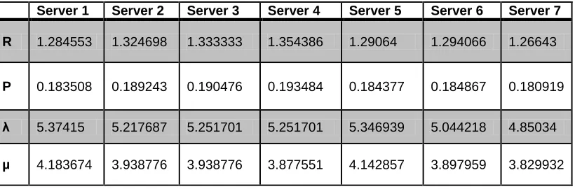
Table 2: Average of the Presented Data in a Week
Server 1 Server 2 Server 3 Server 4 Server 5 Server 6 Server 7
R 1.284553 1.324698 1.333333 1.354386 1.29064 1.294066 1.26643
P 0.183508 0.189243 0.190476 0.193484 0.184377 0.184867 0.180919
λ 5.37415 5.217687 5.251701 5.251701 5.346939 5.044218 4.85034
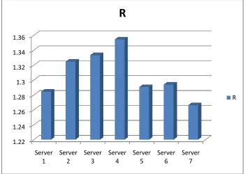
Table 1: Column Chart Analysis for average number of customers being served in a week
The column chart showed the same average number of customers being served on each of the servers experimented in the week. From the result, it was observed
that Server 4 has the highest average number of customers being served, while Server 7 has the lowest average number of customers being served.
Figure 2: Column Chart System Utilization in a Week 1.22
1.24 1.26 1.28 1.3 1.32 1.34 1.36
Server 1
Server 2
Server 3
Server 4
Server 5
Server 6
Server 7
R
R
0.174 0.176 0.178 0.18 0.182 0.184 0.186 0.188 0.19 0.192 0.194
Server 1 Server 2 Server 3 Server 4 Server 5 Server 6 Server 7
P
The line chart showed the average daily system utilization for the seven servers experimented in the week. From the result, it was observed that server 4 has the highest average system utilization, while server7 has the lowest average system utilization.
Figure 3: Average Column Chart Arrival Rate of the Customers in a week
The column chart showed the average daily arrival rate for the seven servers experimented in the week. From the result, it was observed that server 1 has the highest average number of arrival rate, while server 7 has the lowest average number of arrival rate.
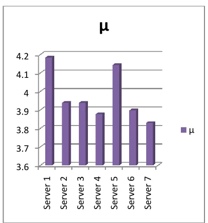
Figure 4: Average Column Chart Service Rate of the Customers in a week
In figure 4, the column chart showed the average daily service rate for the seven servers experimented in the week. From the result, it was observed that server 1 has the highest average number of service rate, while server 7 has the lowest average number of service rate.
The average number of customers being served
𝑅 =𝜆
𝜇 (1)
System Utilization for the Channels
𝜌 = 𝜆
𝑀 𝜇 (2)
The system capacity = Μ𝜇 (3)
Use the models below in excel for the development of the P0 and Lq models to arrive at the average number of
customers being served in the queuing system and the development of other results of a multiple channels single line queuing system.
Probability of zero units in the system(𝑃0)
𝑃0 =
𝜆 𝜇 𝑛 𝑛 ! 𝑀−1 𝑛=0 + 𝜆 𝜇 𝑀
𝑀! 1−𝑀𝜇𝜆 −1
(4)
Table 4 below showed the results of P0 and Lq models
developed in NNPC MEGA Station for Petroleum queuing system. System Utilization is the ratio of system capacity used to available capacity. It measures the average time the system is busy. Probability of n in the system (Pn): This
is the probability that there are exactly n entities in the system (queue and serving mechanism together) at a point in time. Mean Number in Queue (Lq): Mean number in the queue is the average or expected number of system users (patients) in the queue (waiting line), waiting for their turn to be served. Table 4 is building on the following assumption:
1. that all servers work at the same average rate, 2. a poisson arrival rate and exponential service time, 3. customers form a single waiting line and
4. the table is build based on trial and error, to understand, the actual point were the appropriate number of servers will take the give average awaiting line (Lq) and probability. At that point, we also get the actual system utilization that serves the systems. Table 3 was used for the analyses of the results.
Average number in line
Lq=
𝜆𝜇 𝜇𝜆 𝑀
𝑀−1 ! 𝑀𝜇 −𝜆 2 𝑃0 (5)
𝑃0 = Probability of zero units in the system µ= Average Service Rate for the Three Servers λ= Average Customers arrival rate for the three servers 𝜆
𝜇 = The average number of customers being served(R)
𝑛 = Number of units
Average waiting time for an arrival not immediately served
𝑊𝑎
𝑊𝑎 = 1
𝑀𝜇 − 𝜆 (6)
Probability that an arrival will have to wait for service (𝑃𝑤)
𝑃𝑤 = 𝑊𝑞
𝑊𝑎 (7)
The average time customers wait in line (𝑊𝑞)
𝑊𝑞 = 𝐿𝑞
𝜆 (8)
The Average Number of Customers in the System (waiting and /or being served)
𝐿𝑆= 𝐿𝑞+ 𝑅 (9)
Or 𝐿𝑆= 𝑊𝑠 × 𝜆 (10)
The average time spend in the system (waiting in line and service time) (𝑊𝑠)
𝑊𝑠= 𝑊𝑞+ 1 𝜇 =
𝐿𝑠
𝜆 (11)
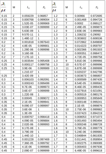
Using equations (4) and (5) above, we have the results in the table 3 below
Table 3: Table Presentation and Analysis of Shoprite Data
M 𝐿𝑞 𝑃0 M 𝐿𝑞 𝑃0
0.15 2 0.059229 0.96857 1.2 5 0.00966 0.972695 0.15 3 0.000768 0.999004 1.2 6 0.001468 0.994726 0.15 4 1.52E-05 0.999969 1.2 7 0.0002 0.999127 0.15 5 3.03E-07 0.999999 1.2 8 2.49E-05 0.999873
0.15 6 5.63E-09 1 1.2 9 2.83E-06 0.999983
0.15 7 9.57E-11 1 1.3 2 1.336232 0.29092
0.15 8 1.48E-12 1 1.3 3 0.303602 0.606536
0.2 3 0.001818 0.997643 1.3 4 0.072862 0.849808 0.2 4 4.8E-05 0.999901 1.3 5 0.014223 0.959797 0.2 5 1.28E-06 0.999996 1.3 6 0.002366 0.991503
0.2 6 3.16E-08 1 1.3 7 0.000351 0.998472
0.2 7 7.17E-10 1 1.3 8 4.72E-05 0.999758
0.25 3 0.003544 0.995408 1.3 9 5.81E-06 0.999966 0.25 4 0.000117 0.999758 1.3 10 6.57E-07 0.999996 0.25 5 3.9E-06 0.999989 1.3 11 6.87E-08 0.999999
0.25 6 1.21E-07 1 1.4 5 0.020237 0.942796
0.25 7 3.42E-09 1 1.4 6 0.003673 0.986807
0.3 3 0.006103 0.992091 1.4 7 0.000589 0.997435 0.3 4 0.000243 0.999499 1.4 8 8.54E-05 0.999563 0.3 5 9.7E-06 0.999973 1.4 9 8.46E-05 0.999435 0.3 6 3.6E-07 0.999999 1.5 5 0.027916 0.921091
0.3 7 1.22E-08 1 1.5 6 0.005519 0.980176
0.35 4 0.00045 0.999072 1.5 7 0.000953 0.995849 0.35 5 2.1E-05 0.999941 1.5 8 0.000148 0.999241 0.35 6 9.09E-07 0.999997 1.5 9 2.1E-05 0.999876
0.35 7 3.6E-08 1 1.5 10 2.75E-06 0.999982
0.35 8 1.3E-09 1 1.6 5 0.037423 0.894219
0.4 4 0.000767 0.998418 1.6 6 0.008053 0.971073 0.4 5 4.09E-05 0.999884 1.6 7 0.001493 0.993494 0.4 6 2.02E-06 0.999993 1.6 8 0.000248 0.998728
0.4 7 9.17E-08 1 1.6 9 3.76E-05 0.999779
0.4 8 3.79E-09 1 1.6 10 5.24E-06 0.999965
0.4 9 1.44E-10 1 1.7 5 0.048844 0.861935
0 . 4 5
8 9.73E-09 1 1.7 10 9.6E-06 0.999936
0.5 4 0.001869 0.996147 1.8 5 0.062164 0.824286 0.5 5 0.000125 0.999648 1.8 6 0.015855 0.943049 0.5 6 7.72E-06 0.999972 1.8 7 0.003377 0.985285 0.5 7 4.37E-07 0.999998 1.8 8 0.000636 0.996744
0.5 8 2.26E-08 1 1.8 9 0.000109 0.999361
0.55 5 0.000201 0.999433 1.8 10 1.7E-05 0.999887 0.55 6 1.37E-05 0.999951 1.9 5 0.077246 0.781653 0.55 7 8.52E-07 0.999996 1.9 6 0.021463 0.922907
0.55 8 4.85E-08 1 1.9 7 0.004898 0.978659
0.55 9 2.52E-09 1 1.9 8 0.000978 0.994991
0.6 5 0.00031 0.999124 1.9 9 0.000176 0.998961 0.6 6 2.31E-05 0.999917 1.9 10 2.92E-05 0.999806 0.6 7 1.57E-06 0.999993 2 5 0.093839 0.73475
0.6 8 9.72E-08 1 2 6 0.028408 0.89796
0.6 9 5.52E-09 1 2 7 0.006949 0.96972
0.65 2 0.713509 0.621372 2 8 0.00147 0.992469 0.65 3 0.020442 0.980131 2 9 0.00028 0.998352 0.65 4 0.001337 0.997796 2 10 4.88E-05 0.999676 0.65 5 9.26E-05 0.999782 2.1 5 0.111588 0.684581 0.65 6 6.21E-06 0.999981 2.1 6 0.036792 0.867843 0.65 7 3.92E-07 0.999999 2.1 7 0.009659 0.957912
0.65 8 2.3E-08 1 2.1 8 0.002164 0.988912
0.7 5 0.00067 0.998108 2.1 9 0.000434 0.997446 0.7 6 5.81E-05 0.999791 2.1 10 7.94E-05 0.999472 0.7 7 4.61E-06 0.99998 2.2 5 0.130066 0.632349 0.7 8 3.34E-07 0.999998 2.2 6 0.046653 0.832423
0.7 9 2.21E-08 1 2.2 7 0.013164 0.942641
0.75 5 0.000945 0.99733 2.2 8 0.003125 0.983993 0.75 6 8.79E-05 0.999684 2.2 9 0.000658 0.996123 0.75 7 7.47E-06 0.999967 2.2 10 0.000126 0.999159 0.75 8 5.79E-07 0.999997 2.3 5 0.148821 0.579336
0.75 9 4.11E-08 1 2.3 6 0.057945 0.791862
0.8 5 0.001303 0.996317 2.3 7 0.0176 0.92331 0.8 6 0.00013 0.999535 2.3 8 0.004429 0.977313 0.8 7 1.17E-05 0.999949 2.3 9 0.00098 0.994227 0.8 8 9.71E-07 0.999995 2.3 10 0.000197 0.998689
0.8 9 7.35E-08 1 2.4 5 0.167412 0.526787
0.95 3 0.155878 0.797985 2.6 9 0.002922 0.982798 0.95 4 0.023278 0.952017 2.6 10 0.00067 0.995545 0.95 5 0.003062 0.991346 2.7 6 0.113459 0.592457 0.95 6 0.000363 0.998697 2.7 7 0.046658 0.796699 0.95 7 3.91E-05 0.99983 2.7 8 0.015081 0.922747 0.95 8 3.84E-06 0.99998 2.7 9 0.004075 0.976007 0.95 9 3.45E-07 0.999998 2.7 10 0.000975 0.993516 1 2 1.112845 0.409462 2.8 6 0.128369 0.538903 1 3 0.175897 0.77204 2.8 7 0.056834 0.752356 1 4 0.02827 0.941726 2.8 8 0.01966 0.899287 1 5 0.003947 0.988844 2.8 9 0.005601 0.967022 1 6 0.000493 0.998228 2.8 10 0.001398 0.990698
1 7 5.6E-05 0.999756 2.9 6 0.143 0.486348
1 8 5.79E-06 0.99997 2.9 7 0.067972 0.703825 1 9 5.48E-07 0.999997 2.9 8 0.02521 0.870861
1 10 4.76E-08 1 2.9 9 0.007588 0.955322
1 11 3.83E-09 1 2.9 10 0.001978 0.986839
1.1 5 0.006313 0.982155 3 6 0.157059 0.435848 1.1 6 0.000873 0.996864 3 7 0.079844 0.652097 1.1 7 0.000109 0.999525 3 8 0.031785 0.837178 1.1 8 1.24E-05 0.999936 3 9 0.010134 0.940333 1.1 9 1.29E-06 0.999992 3 10 0.002762 0.981626
Using Equations 1 to 11 and Table 3 above the Charts below where developed
Figure 5: Column Chart System Utilization for the Multiple Channels
In figure 5, the column chart was used to analyze the system utilization of Shoprite queuing system in Enugu state. The chart was used to understand the utilization of the queuing system for every fifteen minutes of the time in the queuing system.
Figure 6: Line Chart System Utilization for the Multiple Channels
In figure 6, the column chart was used to analyze the system utilization of Shoprite queuing system in Enugu state. The chart was used to understand the utilization of the queuing system per hour. From the chart, the system observed that multiple server of two (2) were been utilized by 131% approximately. However multiple servers 3 and 4 were utilized at 87% and 65% respectively. Also, multiple servers of 5, 6 and 7 were also utilized at 52%, 44% and 37% respectively. On the other hand, multiple servers of 8, 9, 10 and 11 were also utilized at 33%, 29%, 26% and 24% respectively.
0 0.1 0.2 0.3 0.4 0.5 0.6 0.7
1 3 5 7 9
System Utilization
ρ
System Utilization ρ
0 0.2 0.4 0.6 0.8 1 1.2 1.4
1 3 5 7 9
System Utilization
PER HOUR ρ
Figure 7: Column Chart Analysis that Shows the Probability that the System is Empty
In figure 7, the column chart was used to analyze the probability of zero units for Shoprite plaza, Enugu state. The chart was use to show the probability of having zero units in the system before queuing and the probability runs from zero to one or zero percent to hundred percent. The chart was used to understand the probability of zero units in the queuing system.
Figure 8: Line Chart Analysis Which Shows the Probability that the Arrival Must Wait
In figure 8, the line chart was used to analyze the probability that the arrival must wait before being served. When the chart goes towards zero, it shows that the probability of waiting is zero in the queuing system.
Figure 9: Column Chart Analysis Which Shows the Average Number in Line
In figure 9, the line chart shows the average number of customers in the line. The result shows that as the number of servers increases, the number of customers in the queue decreases until it reach to the optimum number of servers that can utilize the queue line and has zero queue in the line.
Figure 10: Column Chart Analysis Which Shows the Average Number in System
In figure 10, the column chart shows the average number of customers in the system. The result shows that as the number of servers increases, the number of customers in the queue decreases until it reach to the optimum number of servers that can utilize the queue system. Note also that the average number of customers in the system tends to one (i.e. the person being served) in the system.
0 0.2 0.4 0.6 0.8 1
1 3 5 7 9
Probability that the
System is empty Po
Probability that the System is empty Po
0 0.2 0.4 0.6 0.8
1 3 5 7 9
Probability that the
arrival must wait Pw
Probability that the arrival must wait Pw
0 0.5 1 1.5
1 3 5 7 9
Average number in
Line Lq
Average number in Line Lq
0 1 2 3
1 3 5 7 9
Average number in
System Ls
Figure 11: Column Chart Analysis Which Shows the Average Time in Line
In figure 11, the column chart shows the average time the customers have to wait in line before being served. The time decreases as the number of servers increases.
Figure 12: Column Chart Analysis Which Shows the Average Time in System
In figure 12, the column chart shows the average time the customers have to wait in the system before being served. The time to wait in the system decreases as the number of servers increases.
Figure 13: Column Chart Analysis Which Shows the Average Waiting Time
In figure 13, the column chart shows the Average waiting time for an arrival not immediately served. The time to wait decreases as the number of servers increases. This shows that the increase in servers will reduce waiting time.
Figure 14: Column Chart Analysis that Detailed the General Analysis of the Queuing Systems
In figure 14, line chart analysis shows the general detailed information and analysis of the queuing system in the Shoprite plaza Enugu State.
0 0.05 0.1 0.15 0.2 0.25 0.3
1 3 5 7 9
Average Time in Line
Wq
Average Time in Line Wq
0 0.1 0.2 0.3 0.4 0.5 0.6
1 3 5 7 9 11
Average Time in System
Ws
Average Time in System Ws
0 0.05 0.1 0.15 0.2 0.25 0.3 0.35 0.4
1 3 5 7 9
Average Waiting Time
Wa
Average Waiting Time Wa
0 0.5 1 1.5 2 2.5 3
1 2 3 4 5 6 7 8 9 10
System Utilization ρ
Probability that the System is empty Po
Probability that the arrival must wait Pw
Table 4: Results for Shoprite Queuing System Analysis
No of Servers
System Utilizatio n
Probabilit y System is empty
Probability arrival must wait
Average number in Line
Average number in System
Average Time in Line
Average Time in System
Average Waiting Time
System Utilizatio n per hour
M Ρ Po Pw Lq Ls Wq Ws Wa ρ
2 0.653315 0.29092 0.70908 1.336232 2.642861 0.257415 0.509127 0.363027 1.306629
3 0.435543 0.606536 0.393463 0.303602 1.610231 0.058487 0.310199 0.148646 0.871086
4 0.326657 0.849808 0.150191 0.072862 1.379491 0.014036 0.265749 0.093456 0.653315
5 0.261326 0.989625 0.040203 0.014223 1.320852 0.00274 0.254452 0.068152 0.522652
6 0.217772 0.991503 0.008499 0.002366 1.308995 0.000456 0.252168 0.053631 0.435543 7 0.186661 0.998472 0.001529 0.000351 1.30698 6.76E-05 0.25178 0.044211 0.373323
8 0.163329 0.999758 0.000242 4.72E-05 1.306676 9.09E-06 0.251721 0.037606 0.326657
9 0.145181 0.999966 3.42E-05 5.81E-06 1.306635 1.12E-06 0.251713 0.032718 0.290362 10 0.130663 0.999996 4.37E-06 6.57E-07 1.30663 1.27E-07 0.251712 0.028955 0.261326
11 0.118784 0.999999 5.1E-07 6.87E-08 1.306629 1.32E-08 0.251712 0.025967 0.237569
Discussion and Conclusion:
From the analysis and results, figure 6 was chart that represents the rate of system utilization per hour in the Shoprite station queuing system in Enugu State. From the chart, the system observed that multiple server of two (2) were been utilized by 131% approximately. However multiple servers 3 and 4 were utilized at 87% and 65% respectively. Also, multiple servers of 5, 6 and 7 were also utilized at 52%, 44% and 37% respectively. On the other hand, multiple servers of 8, 9, 10 and 11 were also utilized at 33%, 29%, 26% and 24% respectively. In figure 7, the probability of zero unit chart was use to analyze the probability of having an empty queuing system before the initial first second on the queuing system. From the results, as the number of servers increase, the probability of zero units also increases to unity (i.e. 1). The unity of the zero probability tells that the probability of having an empty system at initial is 100% and that the probability runs from zero to one or zero percent to hundred percent. However, the charts were used to understand the probability of zero units in the queuing system. In figure 8, there charts were use to analyze the probability that the arrival must wait before being served. When the chart goes towards zero as the number of channels increases, it shows that the probability of waiting is tending towards zero in the queuing system. In figure 9, there chart shows the average number of customers in line that wait to be served. The charts show that as the number of servers increase, the average number of customers waiting to be served in line will tend to zero number of customers in queue. Figure 10, was use to show the charts of the average number of customers in the system. The charts show that as the number of servers increases in the system, the average number of customers will decrease and tends to one (i.e. the customer being served) in the system. Figure 11 shows the average time the customers have to wait in line before being served. The time decreases as the number of servers increases. Figure12 shows the average time the customers have to wait in the system before being served. The time to wait in
the system decreases as the number of servers increases. In figure13, the charts observe the average waiting time for an arrival not immediately served. The time to wait decreases as the number of servers increases. Figure 14 was used to observe the chart analysis which shows the general detailed information and analysis of the queuing system in Shoprite Enugu State. From the analysis, it was observed that number of servers necessary to serve the customers in the case study establishment was six (6) servers (or channels). This was proved in table 4 above. This is the appropriate number of servers that can serve the customers as and at when due without waiting for long before customers are been served at the actual time necessary for the service.
Conclusion:
The evaluation of queuing system in an establishment is necessary for the betterment of the establishment. As it concerns the case study company, the evaluation or analysis of their queuing system shows that the case study company needs to decrease the number of their channels or servers. The Shoprite Station Enugu needs to reduce the number of servers up to six (6) servers in other to utilize the queuing system. The decrease in the number of servers will reduce the time customers have to wait in line before been served. This will also increase the efficiency of the establishment due to the appreciation in their service to the customers as and at when due.
Reference
[1]. Sundarapandian, V. (2009). "7. Queueing Theory". Probability, Statistics and Queueing Theory. PHI Learning. ISBN 8120338448.
[3]. Hall, R. W.: Queueing Methods: For Services and Manufacturing, Prentice-Hall, Upper Saddle River, NJ, 1991.
[4]. Lawrence W. Dowdy, Virgilio A.F. Almeida, Daniel A. Menasce (Thursday Janery 15, 2004). "Performance by Design: Computer Capacity Planning By Example". p. 480
[5]. Schlechter, Kira (Monday March 02, 2009). "Hershey Medical Center to open redesigned emergency room". The Patriot-News
[6]. Mayhew, Les; Smith, David (December 2006). Using queuing theory to analyse completion times in accident and emergency departments in the light of the Government 4-hour target. Cass Business School. ISBN 978-1-905752-06-5. Retrieved 2008-05-20.
[7]. Tijms, H.C, Algorithmic Analysis of Queues", Chapter 9 in A First Course in Stochastic Models, Wiley, Chichester, 2003
[8]. "Agner Krarup Erlang (1878 - 1929) | plus.maths.org". Pass.maths.org.uk. Retrieved 2013-04-22.
[9]. Asmussen, S. R.; Boxma, O. J. (2009). "Editorial introduction". Queueing Systems 63: 1. doi:10.1007/s11134-009-9151-8. edit
[10]. Stidham, S., Jr.: ―Analysis, Design, and Control of Queueing Systems,‖ Operations Research, 50: 197–216, 2002.