SRef-ID: 1684-9981/nhess/2004-4-277
© European Geosciences Union 2004
and Earth
System Sciences
A long range dependent model with nonlinear innovations for
simulating daily river flows
P. Elek and L. M´arkus
Department of Probability Theory and Statistics, E¨otv¨os Lor´and University, Budapest, Hungary
Received: 30 September 2003 – Revised: 11 February 2004 – Accepted: 5 March 2004 – Published: 16 April 2004 Part of Special Issue “Multidisciplinary approaches in natural hazards”
Abstract. We present the analysis aimed at the estimation of
flood risks of Tisza River in Hungary on the basis of daily river discharge data registered in the last 100 years. The deseasonalised series has skewed and leptokurtic distribu-tion and various methods suggest that it possesses substantial long memory. This motivates the attempt to fit a fractional ARIMA model with non-Gaussian innovations as a first step. Synthetic streamflow series can then be generated from the bootstrapped innovations. However, there remains a signifi-cant difference between the empirical and the synthetic den-sity functions as well as the quantiles. This brings attention to the fact that the innovations are not independent, both their squares and absolute values are autocorrelated. Furthermore, the innovations display non-seasonal periods of high and low variances. This behaviour is characteristic to generalised au-toregressive conditional heteroscedastic (GARCH) models. However, when innovations are simulated as GARCH pro-cesses, the quantiles and extremes of the discharge series are heavily overestimated. Therefore we suggest to fit a smooth transition GARCH-process to the innovations. In a standard GARCH model the dependence of the variance on the lagged innovation is quadratic whereas in our proposed model it is a bounded function. While preserving long memory and elim-inating the correlation from both the generating noise and from its square, the new model is superior to the previously mentioned ones in approximating the probability density, the high quantiles and the extremal behaviour of the empirical river flows.
1 Introduction
River Tisza – the second largest in Hungary – has a long his-tory of damaging floods even after the river was controlled in the nineteenth century. The record water levels in years 2000 and 2001 drew again the attention to the question how high Correspondence to: P. Elek
dams should be built in order to prevent a huge flood catastro-phe in the Great Hungarian Plain. So the estimation of high quantiles of the discharge series has again become crucial. Beyond that, studying the behaviour of the whole process is also important because the river provides irrigation water for a large agricultural area in the Hungarian Plain. In the past, the extremal analysis and the conventional time series analysis for River Tisza were usually carried out in separate studies. This paper attempts to incorporate both approaches: the aim is to find a time series model which describes both the regular and the extremal behaviour of the process.
The data we have at our disposal consists of daily wa-ter discharges from 1901 to 2000 at six monitoring stations along the river (Tivadar, V´as´arosnam´eny, Z´ahony, Polg´ar, Szolnok and Szeged). To obtain a visual impression of the data, we display on Fig. 1 the discharge series registered at V´as´arosnam´eny station. It turns out that all six series exhibit a substantial linear and seasonal trend both in their mean and their variance. We used a classical approach to tackle this problem: first a linear and a periodic trend component was subtracted from the data at each station and then these mean-corrected series were standardised by a periodic factor to make the variance roughly constant over time. The periodic components were estimated using the loess smoother proce-dure proposed by Cleveland et al. (1990). The drawback of this procedure is that the standardised series – although sta-tionary in mean and variance – still exhibit seasonal change in their probability density functions. We will see that this problem can partly be resolved during simulations.
0
1000
2000
3000
4000
year
water discharge
1901 1921 1941 1961 1981 2000
Fig. 1. Daily discharge series at V´as´arosnam´eny (m3/s),
1901–2000.
with this phenomenon. For a recent example see Montanari et al. (1997) and for a monograph see Beran (1994).)
Although this simulation method gives back the autocorrelation-structure of the water discharge series of River Tisza accurately, it is not suitable for flood risk estimation because the high quantiles of the synthetic series remain well below the empirical ones. The reason is that the innovations of the fractional ARIMA model – which are non-Gaussian – are uncorrelated but not independent. This phenomenon is consistent with the fact that hydrologic time series are highly nonlinear, so a linear model may not give back the whole complexity of the process.
Innovations can be regarded as shocks to the linear system. They are uncorrelated but their squares and absolute values are autocorrelated and, additionally, they exhibit nonseasonal periods of high and low variances with high variance gener-ally occuring during unusual weather events. These proper-ties suggest modelling the innovations with a variant of the standard GARCH process. (GARCH processes were intro-duced by Bollerslev in 1986 and since then have been widely used especially in financial mathematics.) However, as hy-drologic time series are less heavy-tailed than financial ones, the models should differ as well. In a standard GARCH pro-cess the dependence of the variance on the lagged innova-tions is quadratic, whereas in our model it is a bounded func-tion.
Our approach for simulation is thus the following: we fit a GARCH-type model to the innovation series, estimate the GARCH residuals and then use a resampling procedure to simulate them. In doing so, we take into consideration the seasonally changing shape of their probability density as well. We then apply the GARCH model to get back the inno-vations of the linear system. Finally we drive the fractional ARIMA filter with the innovations and use the seasonal
com-Table 1. Results of fractional ARIMA fit
Monitoring station p q Hurst-parameter p-value
Tivadar 1 1 0.748 (0.022) 0.893
V´as´arosnam´eny 2 1 0.821 (0.014) 0.759
Z´ahony 2 1 0.804 (0.018) 0.738
Polg´ar 2 1 0.794 (0.026) 0.451
Szolnok 2 3 0.752 (0.034) 0.051
Szeged 2 2 0.844 (0.030) 0.057
ponents to obtain synthetic streamflow series. This model, by incorporating time-varying nonseasonal variance, estimates the probability density and high quantiles of the observed se-ries much better than a linear model. It brings us closer to understanding the nonlinear nature of hydrologic time series.
2 Fitting a fractional ARIMA model
In view of the long memory property we first fitted the series with a fractional ARIMA (FARIMA) processXtsatisfying
8p(B)(1−B)dXt =9q(B)εt. (1)
HereBis the backward shift operator,dis the order of frac-tional differencing,εt is the uncorrelated and zero-mean
in-novation (noise) sequence with varianceσε2, and, in the no-tations of ARMA-methodology,
8p(B)=1−
p X
j=1
φjBj (2)
9q(B)=1+
q X
j=1
ψjBj. (3)
In cases of our interestd lies within 0 and 0.5. The Hurst-parameter is thenH=d+1/2.
A FARIMA(p,d,q)model hasp+q+2 parameters: p+q
for the ARMA-coefficients, one for the fractional differenc-ing parameter (these together are called the structural param-eters) and one for the variance of the innovation process. In the following, we denote the structural parameters byθ. The parameters can be estimated by various methods, in-cluding exact normal-based maximum likelihood procedure or the Whittle-estimator. The latter, which we used, is essen-tially an approximation of the log-likelihood function in the spectral domain. According to Giraitis and Surgailis (1990), the Whittle-estimator is consistent and asymptotically nor-mal for linear processes with finite fourth moment. However, these properties cease to hold for certain nonlinear processes, see e.g. Giraitis and Taqqu (1999).
−2 −1 0 1 2
0
2
4
6
8
innovation
probability density
Fig. 2. Probability density of innovations at V´as´arosnam´eny.
asymptotically normal and thus a p-value can easily be calcu-lated. For model identification (i.e. choosing the appropriate value ofpandq) we used a trial and error procedure and then evaluated the different models by the p-value of the goodness of fit statistics and by the significance level of the parameters. Table 1 shows the most important features of the finally fitted models at all sites. As the values with the standard errors (in parentheses) show, the Hurst-parameters significantly exceed 0.5, implying long memory in all cases.
According to the p-values in the table, all six models are acceptable at 5% significance level. (The lower p-values at Szolnok and Szeged are most probably resulted from the fact that reservoirs are operated just upstream of these stations.) The good fit is also expressed by the uncorrelatedness of in-novations at all stations. In other words, the linear model fully describes the linear dependence structure, that is, the autocovariances of the series. The innovations were obtained using a finite approximation of the inverse of the estimated FARIMA filter:
˜
εt =9q(B)−18p(B)(1−B)dXt ≈ 200 X
j=0
bjXt−j. (4)
3 Simulations from the fractional ARIMA model
Nevertheless, from the natural hazards (flood) perspective, the main question is the linear model’s goodness of fit in terms of distribution and high quantiles. To examine that, we need to simulate water discharge series from the model. If the independence of innovations is assumed, the simulation can be carried out in the following straightforward way.
First, synthetict innovations are generated. As their
dis-tribution is highly non-Gaussian (see Fig. 2), a seasonal boot-strap procedure is applied: a synthetic innovation in month A is randomly selected from all observed innovations in the same month of a possibly different year. This method (used e.g. by Montanari et al., 1997) has the advantage of not mak-ing any artificial distributional assumptions, but it has some
0 1000 2500
0.000
0.002
0.004
Tivadar
water discharge
0 2000 4000
0.0000
0.0015
Vasarosnameny
water discharge
0 2000 4000
0.0000
0.0010
0.0020
Zahony
water discharge
0 2000 4000
0.0000
0.0010
0.0020
Polgar
water discharge
0 1000 2500
0.0000
0.0010
Szolnok
water discharge
0 2000 4000
0 e+00
6 e−04
Szeged
water discharge
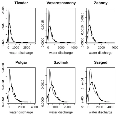
Fig. 3. Probability density of observed (continuous line) and of
lin-early simulated (dashed line) discharge series (in m3/s) at different stations.
serious drawbacks, being very sensitive to extreme observa-tions.
In the second step,Xtis obtained fromtusing the moving
average representation of fractional ARIMA processes. In practise, we used innovations up to lag 200:
Xt =(1−B)−d8p(B)−19q(B)εt ≈ 200 X
j=0
ajεt−j. (5)
Finally, giving back the seasonal components (both in mean and variance) toXt, synthetic water discharge series
are generated.
● ● ●
●●
500
1500
2500
3500
Tivadar
probability (%)
90 99 99.9 100
●
● ●
● ●●
1000
2000
3000
4000
Vasarosnameny
probability (%)
90 99 99.9 100
● ●
● ●
● ●●
1000
2000
3000
Zahony
probability (%)
90 99 99.9 100
● ●
● ●
●
1500
2500
3500
Polgar
probability (%)
90 99 99.9 100
● ●
● ●●
1500
2500
Szolnok
probability (%)
90 99 99.9 100
●
●
● ●
● ●●
2000
3000
4000
Szeged
probability (%)
90 99 99.9 100
● ● ●
●
● ● ●
Fig. 4. Boxplots of quantiles, displayed at 90, 95, 99, 99.5, 99.9,
99.95% levels, and of sample maxima of 20 simulated series at each site, compared to the observed values (circles). Boxplots contain the median value, the quartiles and the extreme observations.
0 10 20 30 40
0.0
0.2
0.4
0.6
0.8
1.0
Lag Tivadar
0 10 20 30 40
0.0
0.2
0.4
0.6
0.8
1.0
Lag Vasarosnameny
0 10 20 30 40
0.0
0.2
0.4
0.6
0.8
1.0
Lag Zahony
0 10 20 30 40
0.0
0.2
0.4
0.6
0.8
1.0
Lag Polgar
0 10 20 30 40
0.0
0.2
0.4
0.6
0.8
1.0
Lag Szolnok
0 10 20 30 40
0.0
0.2
0.4
0.6
0.8
1.0
Lag Szeged
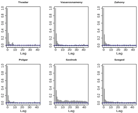
Fig. 5. Autocorrelation function of squared innovations at different
sites.
4 Incorporating the structure of innovations
The above described model has one point at which it fails: it does not incorporate the nonlinear dependence structure of the innovations. As evidenced by Figs. 5 and 6, the innova-tions are dependent through their squares and their absolute values. (The autocorrelatedness of the squared and the abso-lute valued innovation series, respectively, can be proven by a Ljung-Box-test at all reasonable significance levels.) Gen-erating innovations by bootstrap procedure eliminates inter-dependence, thus important information on higher order de-pendence is lost.
Fig. 6. Autocorrelation function of absolute values of innovations
at different sites.
When taking a closer look at the structure of the innova-tions, one can observe that it is a conditionally heteroscedas-tic process: periods of high variance are followed irregularly by less variable periods. This heteroscedasticity is beyond seasonal variation because the latter was eliminated in the standardization procedure. The phenomenon can be called “variance clustering” because innovations with high absolute values (i.e. with high conditional variance) tend to appear in clusters. The clustering also explaines why the squared inno-vation series is autocorrelated.
To demonstrate the clustering effect, we can estimate the variance at time t by the method of moving averages, i.e. by averaging the squared values of innovations from time
t−M/2 until timet+M/2 (here we use the fact that the mean is close to zero):
V ar(ε)t =
1
M+1
M/2 X
j=−M/2
ε2t−j. (6)
When we take e.g.M=10 for a 10 years long subseries, as on Fig. 7, the estimated variance process of the original innova-tion series differs substantially in quantiles and in maximum from that of an independent series obtained by reshuffling. For instance, at V´as´arosnam´eny, the maximum of the former exceeds the maximum of the latter by 38%. This underscores the importance of modelling the clustering effect.
5 Fitting a FARIMA-GARCH model
Series exhibiting variance clustering and other related prop-erties are quite common in empirical finance. They are usually modelled by heteroscedastic processes, of which GARCH-type models are the most widespread. The origi-nal GARCH model was introduced by Bollerslev (1986) and can be formulated in the following way:
0 2000
0.0
0.2
0.4
0.6
0.8
1.0
days
estimated variance
0 2000
0.0
0.2
0.4
0.6
0.8
1.0
days
Fig. 7. A section of the estimated variance process of innovations
(left) and of reshuffled innovations (right) at V´as´arosnam´eny.
σt2=a0+a1εt2−1+b1σt2−1, (8)
where Zt-s are independent, zero-mean random variables
with unit variance, and σt2 is the time-varying conditional variance of εt. a0, a1 andb1 are nonnegative parameters,
which describe the dependence ofσt2 on the lagged value and on the lagged variance. (When b1=0, we obtain the
ARCH model introduced by Engle (1982).) Values of the
εt process are uncorrelated but interdependent through their
squares. A comprehensive introduction into GARCH models is given e.g. in Hamilton (1994).
Because of its inherent heavy-tailedness (Mikosch and Starica, 2000), the above described original GARCH model is not directly suitable for river flow analysis. Instead, a more flexible heteroscedastic GARCH-type model can be used for modelling innovations, where the conditional variance is al-lowed to depend on the lagged values and on the lagged vari-ance in a more complicated way (f is a given parametric bivariate function):
εt =σtZt (9)
σt2=f (εt−1, σt2−1). (10)
Although B¨uhlmann and McNeil (2002) gives a general nonparametric method to identifyf, we have not used this method because of computational difficulties. However, there is an easier – although not precise in the case ofb16=0 – way to illustrate howσt2 depends onεt−1. If the
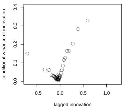
innova-tions are grouped (e.g. into 50 groups) according to their rank and the variance of the subsequent innovations are computed for all groups, we see that their conditional variance depends on the value of the previous innovation (cf. Fig. 8). (If the
εt process were independent, no pattern would appear.)
Ac-cording to Fig. 8, when the absolute value of the innovation is large, we expect the next innovation to have large absolute value as well. However, this empirical relation is far from the quadratic function obtained from the standard GARCH model.
●
● ● ●●●●●●●●●●●●●●●●●●●●●●●●●●●●●●●●●●
●●●● ● ●●
●● ●
● ●
−0.5 0.0 0.5 1.0
0.0
0.1
0.2
0.3
0.4
lagged innovation
conditional variance of innovation
Fig. 8. Empirical conditional variance of innovations as a function
of the previous value at V´as´arosnam´eny.
−2 −1 0 1 2
0.1
0.2
0.3
0.4
lagged innovation
conditional variance of innovation
Fig. 9. Conditional variance of innovations from the fitted
theoreti-cal model.
Based on Fig. 8, we have specifiedf (and thus the model) in the following form:
εt =σtZt (11)
σt2=a0+a1(1−exp(−sε2t−1))+b1σt2−1. (12)
How is this model working? When the absolute value of
εt−1 is large,εt−1 has no incremental effect on the
condi-tional variance. In this caseσt2can be viewed as an autore-gressive process:
σt2≈a0+a1+b1σt2−1.
When εt−1 is closer to zero, the process is similar to a
GARCH-process:
σt2≈a0+a1sε2t−1+b1σt2−1,
which in the neighbourhood of zero reduces to
0 10 20 30 40 0.0 0.2 0.4 0.6 0.8 1.0 Lag Original
0 10 20 30 40
0.0 0.2 0.4 0.6 0.8 1.0 Lag Squares
0 10 20 30 40
0.0 0.2 0.4 0.6 0.8 1.0 Lag Absolute values
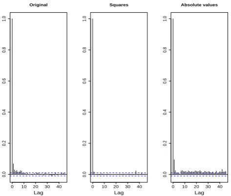
Fig. 10. Autocorrelation function of the original, squared and
abso-lute valued GARCH-residual process at V´as´arosnam´eny station.
As the effect ofεt−1 changes smoothly between these
ex-treme cases, the model may be called a smooth transition GARCH-type process. Put another way, there are basically two distinct regimes in the variance of the innovation pro-cess, and they can transform into one another in a smooth way. The theoretical smooth relationship between the con-ditional variance and the lagged innovations is displayed in Fig. 9.
After the conditional distribution (i.e. the distribution of
Zt) is specified, parameter estimation can be carried out by
the method of conditional maximum likelihood (Hamilton, 1994). In the case of conditional normality, this method es-sentially maximises the following function:
L(a0, a1, b1, s)= n Y
t=1
1
q
2π σt2
exp − ε
2 t
2σt2 !
where σt2is the conditional variance specified in Eq. (12). For the innovations of river discharge at V´as´arosnam´eny the following model was obtained:
εt =σtZt (13)
σt2=0.0062+0.38(1−exp(−3.51ε2t−1))+0.46σt2−1.(14)
6 Simulations from the FARIMA-GARCH model
TheZt series in Eq. (11) (which we call GARCH-residuals)
can be calculated recursively using the expression (14) for
σt2.As Fig. 10 shows, the squared and absolute valued resid-ual process are no longer autocorrelated, although some neg-ligible autocorrelation appears in the residual series itself. So the GARCH-residuals are much closer to independence than the pure innovation process, making simulation by bootstrap-ping more acceptable. As the distribution is more peaked and
0 500 1500 2500
0.0000 0.0005 0.0010 0.0015 0.0020 0.0025 Density function water discharge ● ●●●●●●●●●●● ● ● ● ● ● ● ● ● ● ● ● ● ● ● ● ● ●● ● ● ● ● ● ● ● ● ● ● ● ● ● ● ● ● ● ● ● ● ● ● ● ● ● ● ● ● ● ●●●●●●●●●●●●●●●●●●●●●●●●●●●●●●●●●●●●●●●●●●●●●●●●●●●●●●●●●●●●●●●●●●●●●●●●●●●●●●●●●●●●●●●●●●●●●●●●●●●●●●●●●●●●●●●●●●●●●●●●●●●●●●●●●●●●●●●●●●●●●●●●●●●●●●●●●● ● ● ● ● ● ● ● ● ● 0 1000 2000 3000 4000 5000 6000 7000 Quantiles probability (%) quantile
50 90 99 99.9 100
● ● ● ● ● ● ● ● ● ● ● ● ● ● ● ● ● ● ● ● ● ● ● ● ● ● ● ● ● ● ● ● ● ● ● ● ● ● ● ● ● ● ● ● ● ● ● ● ● ● ● ● ● ● ● ● ● ● ● ● ● ● ● ● ● ● ● ● ● ● ● ● ● ● ● ● ● ● ● ● ● ● ● ● ● ● ● ● ● ● ● ● ● ● ● ● ● ● ● ● ● ● ● ● ● ● ● ● ● ● ● ● ● ● ● ● ● ● ● ● ● ● ● ● ● ● ● ● ● ● ● ● ● ● ● ● ● ● ● ● ● ● ● ● ● ● ● ● ● ● ● ● ● ● ● ● ● ● ● ● ● ● ● ● ● ● ● ● ● ● ● ● ● ● ● ● ● ●
Fig. 11. Probability density and high quantiles (50, 70, 90, 95, 98,
99, 99.5, 99.95% and maximum) of observed (continuous/circled) and simulated (dotted) water discharge series at V´as´arosnam´eny.
heavier-tailed than the standard normal one, the bootstrap procedure is indeed needed again. The shape of the distribu-tion could also cause problems during estimadistribu-tion, however, it is quite common in the finance literature to use Gaussian conditional maximum likelihood even when the distribution is non-Gaussian (see e.g. McNeil and Frey (2000).)
Having simulated the GARCH-residuals, the σt2 condi-tional variances and theεt innovations are easily generated
recursively from Eq. (14). After that, as earlier, the fractional ARIMA filter and the seasonal component can be applied to get synthetic streamflow series.
Figure 11 shows that the peakedness of the probability density is much better approximated by these simulations than by the simulations from the linear model. The 100–year maximum (which is quite important for flood risk estima-tion) is overestimated while quantiles in the range 90%–95% are slightly underestimated. The fit may improve when the generalised Pareto-distribution is used at the tails, or when the form of the model is more carefully chosen, e.g. by the nonparametric fitting procedure proposed by B¨uhlmann and McNeil (2002).
7 Conclusions
forecasting. Seasonal long memory models were analysed recently in Montanari et al. (2000) and Ooms and Franses (2001) where further references can be found.
Our analysis proved that taking into account linear depen-dencies only, no matter at what length or precision, does not result in satisfactory description of the discharge series. This is particularly the case when extremes or high quantiles are concerned. From the numerous possible nonlinear models, a GARCH-type one was selected on the basis of autocor-relations of squares and absolute values and in view of the heteroscedasticity of the innovation process. Heuristic ar-guments for GARCH-innovations – the greater the previous innovation, the larger the variance of the next – may also be given in various possible ways. Were a rigorous connection between the innovations and the flood-generating weather patterns established, one could say: a high-value innovation indicates extreme weather patterns with unstable conditions, leading to high uncertainty in the next step. However, being a guess rather than an argument, we avoid to elaborate on this any further.
The original GARCH-philosophy prescribes the variance conditional on lagged values as a quadratic function. This property is meant to capture investor behaviour in financial markets where incoming shocking news cause greater un-certainty (the above mentioned quadratically increasing vari-ance) for the next couple of days. Natural phenomena lack this psychological effect, therefore in our case there must be a bound for the increase of variance. This is what our modi-fied GARCH-model intends to describe.
There is another way to look at our model. It captures the switch between high and low variance in an easily estimable way, i.e. by making use of the apparent statistical relation-ship between conditional variance and lagged innovations. Whether other processes like regime switching ones may be useful in modelling heteroscedasticity, or, in the GARCH-type context, what other variables the variance may depend on, are topics of further research.
Acknowledgements. This research was funded by Hungarian
National Research and Development Project No. 3/067/2001 (project title: Establishing the Engineering and Scientific Bases of Flood Risk Assessment) and partially by National Scientific Research Fund OTKA, grant No. T 032725.
Edited by: T. Glade Reviewed by: two referees
References
Beran, J.: A goodness of fit test for time series with long-range dependence, J. Roy. Statist. Soc., Series B, 54, 749–760, 1992. Beran, J.: Statistics for long-memory processes, Chapman and Hall,
New York, 1–315, 1994.
Bollerslev, T.: Generalised autoregressive conditional heteroscedas-ticity, J. of Econometrics, 31, 307–327, 1986.
B¨uhlmann, P. and McNeil, A.: An algorithm for nonparametric GARCH modelling, J. of Comput. Statist. and Data Analysis, 40, 665–683, 2002.
Cleveland, B. R., Cleveland, W. S., McRae, J. E., and Terpen-ning, I.: STL: A seasonal trend-decomposition procedure based on loess, J. of Off. Statist., 6, 3–73, 1990.
Engle, R. F.: Autoregressive Conditional Heteroskedasticity with Estimates of the Variance of the United Kingdom Inflation, Econometrica, 50, 987–1007, 1982.
Giraitis, L. and Surgailis, D.: A central limit theorem for quadratic forms in strongly dependent linear variables and applicationto asymptotical normality of Whittle’s estimate, Prob. Th. Rel. Fields, 86, 87–104, 1990.
Giraitis, L. and Taqqu, M. S.: Whittle estimator for finite-variance non-Gaussian time series with long memory, Ann. Statist., 27, 178–203, 1999.
Hamilton, J. D.: Time series analysis, Princeton University Press, Princeton, N.J., 657–676, 1994.
Hurst, H. E.: Long-term storage capacity of reservoirs, Trans. of the Amer. Soc. of Civil Engineers, 770–808, 1951.
Lawrance, A. J. and Kottegada, N. T.: Stochastic modelling of river flow time series, J. Roy. Statist. Soc., Series A, 140, 1–31, 1977. McNeil, A. and Frey, R.: Estimation of tail-related risk measures for heteroscedastic financial time series: an extreme value approach, J. of Empirical Finance, 7, 271–300, 2000.
Mikosch, T. and Starica, C.: Limit theory for the sample autocor-relations and extremes of a GARCH(1,1) process, Ann. Statist., 28, 1427–1451, 2000.
Montanari, A., Rosso, R., and Taqqu, M. S.: Fractionally differ-enced ARIMA models applied to hydrologic time series: Iden-tification, estimation and simulation, Water Resources Research, 33, 1035–1044, 1997.
Montanari, A., Rosso, R., and Taqqu, M. S.: A seasonal fraction-ally differenced ARIMA model: an application to the Nile River monthly flows at Aswan, Water Resources Research, 36, 1249– 1259, 2000.
Noakes, D. J., Hipel, K. W., McLeod, A. I., Jimenez, C., and Yakovitz, S.: Forecasting annual geophysical time series, Intern. J. of Forecasting, 1, 179–190, 1988.
Ooms, M. and Franses, P. H.: A seasonal periodic long memory model for monthly river flows, Environmental Modelling and Software, 16, 559–569, 2001.
Ray, B.: Modeling long-memory processes for optimal long-range prediction, J. of Time Series Analysis, 14, 511–525, 1993. Vecchia, A. V. and Ballerini, R.: Testing for periodic