A comparative study of stresses of a functionally graded thick sphere under thermo-mechanical loadings by Analytical and Finite Element Methods

(1)

A comparative study of stresses of a

functionally graded thick sphere under

thermo-mechanical loadings by Analytical

and Finite Element Methods

P NAYAK

Ph D Scholar, Department of Mechanical Engineering, Jadavpur University, Kolkata 700032, India Corresponding author: [email protected]

S C MONDAL, A NANDI

Professors, Department of Mechanical Engineering, Faculty of Engineering and Technology, Jadavpur University, Kolkata 700032, India

Abstract: This work aims at a comparative study of the stresses of the general analytical solution of a functionally graded thick sphere with that of the finite element analysis (FEA), considering the properties of the material i.e. modulus of elasticity, thermal expansion coefficient and thermal conductivity, vary with the power-law of radius and Poisson’s ratio remains constant and imposing the third kind thermal boundary conditions, with steady-state unidirectional radial heat conduction and general mechanical boundary conditions. Also, the analytical results of the equivalent stress are compared with that of the finite element analysis (FEA).

Keywords: Functionally graded material; third kind thermal boundary condition; thermo-mechanical stress; finite element analysis (FEA); equivalent stress.

1. Introduction

(2)

(3)

loadings and the pressure and temperature are symmetrical about the axis of the cylinder. Also, the material properties are independent of temperature. [Feng et al.(2013)] formulated an edge-based smoothed finite element method to deal with the thermo-mechanical analyses of functionally graded cylindrical vessels. The problem domain is first discretized into triangular elements, and the edge-based smoothing domains are further formed along the edges of the triangular meshes. In order to improve the accuracy, the stiffness matrices are calculated using the strain smoothing technique in these smoothing domains. The vessels are made of ceramics and metals whose volume fractions vary continuously and radially to a power law. The formulation is straight-forward and no penalty parameters or additional degrees of freedom are utilized. [Jabbari et al. (2015)] developed the general solution of steady-state one dimensional radially symmetric mechanical and thermal stresses and electrical and mechanical displacements for a hollow thick cylinder of fluid-saturated functionally graded poro piezoelectric materials. The general form of thermal and mechanical boundary conditions is considered on the inside and outside surfaces. A direct method is used to solve the heat conduction equation and non-homogenous system of partial differential Navier equations, using complex Fourier series and power law functions method. The material properties depend on the radial variable r and expressed as power law functions. [Jabbari et al. (2016)] developed an exact solution for the equation of two-dimensional transient heat conduction in a hollow sphere made of functionally graded material and piezoelectric layers. Transient temperature distribution, as a function of radial and circumferential directions and time with general thermal boundary conditions on the inside and outside surfaces, is analytically obtained for different layers, using the method of separation of variables and Legendre series. The properties depend on the variable r and expressed as power functions of r.

The purpose of this work is to compare the results of the accurate analytical solution obtained for the thermo-mechanical radial, tangential, and equivalent stresses of a thick sphere made of FGM in [Nayak et al. (2011)] with that of the results obtained by the finite element analysis (FEA) in this paper. However, the accurate analytical solution was already validated in [Nayak et al. (2011)] by substituting the value of the power indices equal to zero with which the method of solution and the results were reduced to those of thick sphere of isotropic-homogeneous materials [Chakrabarty (1998); Noda et al. (2003)]. The properties of the material of the sphere are assumed to be graded in the radial direction based on the power-law index function of radius, to the assumptions made by Giannakopoulos and Suresh (1997). A thick sphere of FGM under a unidirectional steady-state heat conduction with the third kind thermal [Ozisik(1985)] and general mechanical [Chakrabarty (1998)] boundary conditions is considered. With the numerical data in [Nayak et al. (2011)], the finite element analysis (FEA) is performed for the radial stresses and tangential stresses of the thermal, mechanical and thermo-mechanical loadings, separately. Also, the analytical results of the equivalent stress are compared with that of the finite element analysis (FEA).

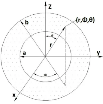
2. Analysis of a functionally graded thick sphere

Fig. 1: A functionally graded thick sphere

To compare the results of the stresses of the accurate analytical solution of a thick sphere made of FGM under thermo-mechanical loadings with that of the results obtained by the finite element analysis (FEA), the governing equations are required. [Nayak et al. (2011)] obtained the required equations of stresses accurately for a functionally graded thick sphere, those are summarized here.

(4)

E

=

E

₀

r

m1

,

α

=

α

₀

r

m2 and

k

=

k

₀

r

m3 (1)

where E0,

α

0 and k0 are material constants for modulus of elasticity E, thermal expansion coefficient

α

and

thermal conductivity k & m1, m2 and m3 are power indices of the material, respectively.

2.1. Temperature distribution of heat transfer problem

Under the steady-state condition, with the heat conduction for the unidirectional spherical co-ordinate and the third kind boundary conditions for a thick sphere as shown in [Ozisik, (1985)], made of functionally graded material, the temperature distribution is given by,

for

m

₃

=

−

1

,

T

=

Z

₁

ln

r

+

Z

₂ (2) and for

m

₃

≠

−

1

, 3₁ ₄

3

Z

r

Z

T

=

_m₊

+

(3)

where T = T(r) is the temperature at any position of r and Z₁, Z₂, Z₃and Z₄are the constants.

2.2. Stress- strain-displacement relationships

As the properties in

φ

and

θ

directions are identical and the symbol udenotes the displacement in the radial direction,

the strain-displacement relationships become,

dr

du

r

=

ε

and

r

u

=

θ

ε

(4)

and the corresponding thermo-elastic stress-strain relationships become ,

σ

_r

=

λ

e

+

2 G

ε

_r

−

(

3 λ

+

2 G

)

α

T

and

σ

_θ

=

λ

e

+

2 G

ε

_θ

−

(

3 λ

+

2 G

)

α

T

(5)

where σr and

ε

r are the stress and strain in radial direction and σθ and

ε

_θ are the stress and strain in tangential

direction, T is rise in temperature with respect to temperature where stress values in the material is zero if the spherical vessel is undeformed, e is the dilatation and λ and G are Lame’s elastic coefficients related with the modulus of elasticity E and Poisson’s ratio ν.

2.3. Equilibrium equation and solution

Neglecting the body force and the inertia, the equilibrium equation becomes

r

(

_r

)

dr

d

r

σ

=

2 _σ

_θ

−

_σ

(6)

First, Eq. (6) converted into displacement u = u(r),

for

m

₃

=

−

1

, ₂ ₁ 1 ₁ 1

2

2 ₂ ₂

ln

Pr

+

Ru

=

M

r

m+

r

+

N

r

m+

dr

du

Qr

dr

u

d

(7)

and for

m

₃

≠

−

1

, ₂ ₂ ₂ 1

2

2 ₂ ₃ ₂

Pr

+

Ru

=

M

r

m−m

+

N

r

m +

dr

du

Qr

dr

u

d

(8)

The general solution of Eq. (7) and (8) are obtained as

for

m

₃

=

−

1

,

u

( )

r

=

X

₁

r

s1

+

X

₂

r

s2

+

(

Y

₁

_ln

r

+

Y

₂

)

r

m2+1₍₉₎

and for

m

₃

≠

−

1

,

u

( )

r

=

X

₃

r

s1

+

X

₄

r

s2

+

Y

₃

r

m2−m3

+

Y

₄

r

m2+1₍₁₀₎

Substituting Eq. (9) into Eq. (4), the strains are obtained as

1 2

[

(

)(

)

]

2

1 2

2 1

1 2 2 1 1

1

ln

1

m s

s

r

=

s

X

r

−

+

s

X

r

−

+

Y

r

+

Y

m

+

Y

r

ε

(11)

and 1 2

(

)

2

2 1

1 2 1

1

ln

m s

s

_X

_r

_Y

_r

_Y

_r

r

X

+

=

− −

θ

ε

(12)

Again substituting Eq. (10) into Eq. (4), the strains are obtained as

1 2

(

)

2 3

(

₁

)

2

2 4 1 3

2 3 1 4 2 1 3 1

m m

m s

s

r

=

s

X

r

−

+

s

X

r

−

+

Y

m

−

m

r

− −

+

Y

m

+

r

(5)

and 1 2 2 3 2 4 1 3 1 4 1 3 m m m s

s

_X

_r

_Y

_r

_Y

_r

r

X

+

=

− − − −

θ

ε

(14)

Now substituting Eq. (11), (12) and (2) into Eq. (5), the stresses are obtained as

( )(

)

( )

{

}

{

( )

}

( )

{

( ) ( )

} ( )

( ) ( )

{

} ( )













+

−

+

−

+

−

+

−

+

−

+

−

+

=

+ + − + − +

r

Z

m

Y

r

Z

m

Y

r

s

X

r

s

X

E

m m m m s m s m r

ln

1

2

1

2

1

2 1 2 1 2 1 1 1 0 1 2 1 0 2 2 2 1 1 2 2 1 1 1 0

α

ν

α

ν

σ

(15)

and

(

)(

)

(

)

(

)

(

) (

)

{

}

(

) (

)

{

}













+

−

+

−

+

−

+

=

+ + − + − +

r

Z

m

Y

r

Z

m

Y

r

s

X

r

s

X

E

m m m m s m s m

ln

1

2

1

2 1 2 1 2 1 1 1 0 1 2 1 0 2 2 2 1 1 2 2 1 1 1 0

α

ν

α

ν

σ

θ (16)

Again substituting Eq. (13), (14) and (3) into Eq. (5), the stresses are obtained as

( )(

)

( )

{

}

{

( )

}

( ) ( )

{

} ( )

( )(

)

{

} ( )













+

−

+

−

+

−

+

−

+

−

+

=

− − + + − + − + 1 0 3 3 2 3 0 4 2 4 1 2 4 1 1 3 0 3 2 1 2 1 2 1 1 1

1

2

1

2

1

2

1

m m m m m s m s m r

r

Z

m

Y

r

Z

m

Y

r

s

X

r

s

X

E

α

ν

α

ν

σ

(17)

and

(

)(

)

(

)

(

)

(

) (

)

{

}

(

)

{

} (

)













+

−

+

−

+

−

+

=

− − + + − + − + 1 0 3 3 2 3 0 4 2 4 1 2 4 1 1 3 0 3 2 1 2 1 2 1 1 1

1

2

1

m m m m m s m s m

r

Z

m

Y

r

Z

m

Y

r

s

X

r

s

X

E

α

ν

α

ν

σ

θ (18)

The mechanical boundary conditions at inside and outside surfaces are considered to find out the constantsX₁,

2

X , X₃ and X₄,from Eq. (15) and (17). The boundary conditions are:

σ

_r

|

_r₌_a

=

−

p

_i and

σ

_r

|

_r₌_b

=

−

p

_o where pi and po are the internal and external fluid pressures respectively. All the constants used above, are

mentioned in Appendix A.

3. Finite element implementation/simulation

Among the numerical methods: the finite difference, the finite element, the boundary element, etc., the finite element method is used in the present analysis. For obtaining the distributions of stresses through the geometry of FG thick sphere subjected to thermo-mechanical loadings, a finite element model is developed using commercially available software ANSYS. Firstly, the thermal model is created and the temperature boundary condition is given and the temperature distribution is calculated. Only one quarter of the cross-section of the sphere is considered with appropriate zero heat flux boundary conditions for symmetry. A quadratic-axisymmetric, eight-node element PLANE 77 is used for this purpose. Along the radial direction eighteen divisions are considered. The thermal conductivity of FG thick sphere is evaluated at the element centroid using the appropriate power law.

Next, the element type is converted from the thermal element PLANE 77 to the mechanical element PLANE 55. PLANE 55 is an axisymmetric element for stress analysis and has same number of nodes as the Plane 77. Appropriate displacement constraints are imposed for the quarter cross-section of the sphere. Just like before, the modulus of elasticity and coefficient of thermal expansion of FG thick sphere are evaluated at the element centroid using the appropriate power law. In this stress analysis part, the temperature distribution is imported from the previously performed thermal analysis (using PLANE 77). Finally, the internal fluid pressure is imposed on the inner layer of the FE model of the sphere and the thermo-mechanical stresses are determined. The analysis steps are implemented using ANSYS Parametric Design Language (APDL).

4. Results and Discussions

[Nayak et al. (2011)] already validated the final equations with substituting zeroes for the indices m1, m2, m3 and

in turn, obtaining the expressions for an isotropic and homogenous sphere those are same as specified in [Chakrabarty, (1998); Noda et al. (2003)]. Again, they also validated the final equations by taking a numerical example (problem) and for the comparative study with the finite element analysis (FEA), the same problem is mentioned below.

Assuming the power indices are same (m1 = m2 = m3 = m), A thick sphere of inside radius, a = 0.8m and outside

(6)

and thermal expansion coefficient are E0= 209.2GPa and α0 = 10.58

×

10-6 /°C, respectively and yield strength

is

σ

_y= 700 MPa. The temperature at inside surface Ta= 20 °C and that at outside surface Tb= 0 °C. The sphere

is subjected to internal pressure, pi of 200 MPa, and external pressure, po of zero (0) and centrifugal heat flux.

For different values of power index m, the radial stresses and the tangential stresses for thermal, mechanical and thermo-mechanical loads are separately treated. For planar isotropy and non-homogeneity in radial direction,

the equivalent stress based on the von Mises criteria is given by

σ

_eq

=

2 (

σ

_θ

−

σ

_r

)

.

4.1. Results obtained by FEA for the radial and tangential stresses at different loadings and power indices

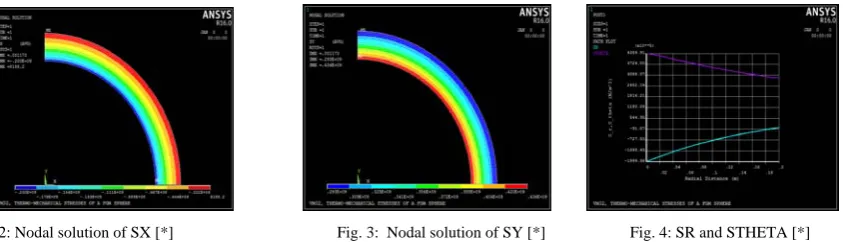
The FEA programme is developed through ANSYS R 16.0 and the results of ANSYS are tabulated below after normalizing the radii by inside radius of the sphere, and the radial and tangential stresses by internal pressure of the fluids i.e. in the path variable summary (the results of ANSYS), when the values of ‘S’ are added with inside radius, 0.8 m, render the position of radii, and the values of ‘SR’ are the radial stresses and that of ‘STHETA’ are the tangential stresses. Again, as a token of the graphical results by ANSYS, the Nodal solution of radial stress [SX], the Nodal solution of tangential stress [SY] as well as the Path plot (graphical plot) of radial stress [SR] and tangential stress [STHETA] for thermo-mechanical loadings are shown in Figs. 2, 3 and 4, respectively, for the power index, m = -2. Similarly, for the rest of the power indices, at different loadings, the graphical results by ANSYS can be generated by running the FEA programme, but avoided without showing them in terms of figures as they are unnecessary, would be similar to Figs. 2, 3 and 4, respectively. However, the numerical results of all the power indices, for thermal, mechanical and thermo-mechanical loadings, by ANSYS, are tabulated in their respective tables, as follows.

Fig. 2: Nodal solution of SX [*] Fig. 3: Nodal solution of SY [*] Fig. 4: SR and STHETA [*]

[*]: SX and SR are Radial stresses, SY and STHETA are Tangential stresses, for thermo-mechanical loadings generated, in ANSYS, for m = -2

4.2. Radial stresses:Comparison of Analytical with FEA results

The analytical results of Radial stresses are obtained from Eq. (15) and (17), those are tabulated below.

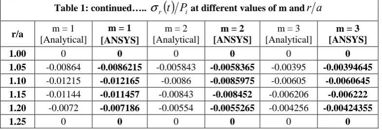
4.2.1. Radial stress for thermal loading: Analytical vs. ANSYS and Percentage (%) difference between Analytical and ANSYS results

Table 1: Analytical and ANSYS results of

σ

_r

( )

t

P

_iat different values of m and

r

a

r/a m = -3

[Analytical]

m = -3 [ANSYS]

m = -2 [Analytical]

m = -2 [ANSYS]

m = -1 [Analytical]

m = -1 [ANSYS]

m = 0 [Analytical]

m = 0 [ANSYS]

1.00 0 0 0 0 0 0 0 0

1.05 -0.04082 -0.0405885 -0.027733 -0.0275995 -0.01882 -0.0187475 -0.01276 -0.012721 1.10 -0.047835 -0.047825 -0.03406 -0.0340605 -0.0242 -0.0242125 -0.017163 -0.017179 1.15 -0.037874 -0.0378995 -0.0282 -0.0281875 -0.021 -0.0209225 -0.0155 -0.0154985 1.20 -0.02024 -0.020221 -0.01567 -0.0156485 -0.012111 -0.0120915 -0.009346 -0.0093329

(7)

Table 1: continued…..

σ

_r

( )

t

P

r

a

r/a m = 1

[Analytical]

m = 1 [ANSYS]

m = 2 [Analytical]

m = 2 [ANSYS]

m = 3 [Analytical]

m = 3 [ANSYS]

1.00 0 0 0 0 0 0

1.05 -0.00864 -0.0086215 -0.005843 -0.0058365 -0.00395 -0.00394645 1.10 -0.01215 -0.012165 -0.0086 -0.0085975 -0.00605 -0.0060645 1.15 -0.01144 -0.011457 -0.00843 -0.008452 -0.006206 -0.006222 1.20 -0.0072 -0.007186 -0.00554 -0.0055265 -0.004256 -0.00424355

1.25 0 0 0 0 0 0

and the correspondingpercentage (%) difference between Analytical and ANSYS results are furnished in

Table 2,

Table 2: Percentage (%) difference between Analytical and ANSYS results for

σ

_r

( )

t

P

_iat different values of m and

r

a

r/a m = -3 m = -2 m = -1 m = 0 m = 1 m = 2 m = 3

1.00 0 % 0 % 0 % 0 % 0 % 0 % 0 %

1.05 0.567 % 0.48% 0.385 % 0.306 % 0.214 % 0.111 % 0.09 % 1.10 0.021 % 0 % 0.052 % 0.093 % 0.1235 % 0.03 % 0.24 % 1.15 0.067 % 0.044 % 0.37 % 0.0097 % 0.15 % 0.261 % 0.258 % 1.20 0.094 % 0.137 % 0.16 % 0.141 % 0.1945 % 0.26 % 0.293 %

1.25 0 % 0 % 0 % 0 % 0 % 0 % 0 %

as well as with the values of the Analytical and ANSYS results in Table 1, the graphical plots of Radial stress for thermal loading based on Analytical results and ANSYS results are shown in Fig. 5and 6, respectively.

Fig. 5: Radial stress for thermal loading [Analytical results] Fig. 6: Radial stress for thermal loading [ANSYS results]

(8)

σ

_r

( )

m

P

r

a

r/a m = -3

[Analytical]

m = -3 [ANSYS]

m = -2 [Analytical]

m = -2 [ANSYS]

m = -1 [Analytical]

m = -1 [ANSYS]

m = 0 [Analytical]

m = 0 [ANSYS]

1.00 -1 -1 -1 -1 -1 -1 -1 -1

1.05 -0.66334 -0.6639 -0.6831 -0.68355 -0.70233 -0.70265 -0.721 -0.7212 1.10 -0.4177 -0.41786 -0.442 -0.44196 -0.46612 -0.466195 -0.4904 -0.490425 1.15 -0.23641 -0.236525 -0.25632 -0.2564 -0.277 -0.276985 -0.2982 -0.29818 1.20 -0.1014 -0.101575 -0.11244 -0.112605 -0.12422 -0.124345 -0.1367 -0.13667

1.25 0 0 0 0 0 0 0 0

Table 3: continued……of

σ

_r

( )

m

P

r

a

r/a m = 1

[Analytical]

m = 1 [ANSYS]

m = 2 [Analytical]

m = 2 [ANSYS]

m = 3 [Analytical]

m = 3 [ANSYS]

1.00 -1 -1 -1 -1 -1 -1

1.05 -0.739 -0.73905 -0.756 -0.75615 -0.77252 -0.77245 1.10 -0.515 -0.5145 -0.5384 -0.53825 -0.56174 -0.5616 1.15 -0.320 -0.31987 -0.342 -0.341925 -0.36438 -0.364225 1.20 -0.150 -0.14984 -0.16355 -0.163515 -0.17784 -0.177735

1.25 0 0 0 0 0 0

Table 4,

Table 4: Percentage (%) difference between Analytical and ANSYS results for

σ

_r

( )

m

P

r

a

r/a m = -3 m = -2 m = -1 m = 0 m = 1 m = 2 m = 3

1.00 0 % 0 % 0 % 0 % 0 % 0 % 0 %

1.05 0.0844 % 0.066% 0.0456 % 0.028 % 0.0068 % 0.02 % 0.0091 % 1.10 0.0383 % 0.009 % 0.0161 % 0.0051 % 0.0971 % 0.028 % 0.025 % 1.15 0.0486 % 0.0312% 0.0054 % 0.0067 % 0.041 % 0.022 % 0.0425 % 1.20 0.1726 % 0.147 % 0.1006 % 0.022 % 0.107 % 0.0214 % 0.05904 %

1.25 0 % 0 % 0 % 0 % 0 % 0 % 0 %

as well as with the values of the Analytical and ANSYS results in Table 3, the graphical plots of Radial stress for mechanical loading based on Analytical results and ANSYS results are shown in Fig.7and 8, respectively.

(9)

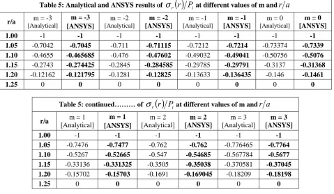
4.2.3. Radial stress for thermo-mechanical loadings: Analytical vs. ANSYS and Percentage (%) difference between Analytical and ANSYS results

σ

_r

( )

r

P

_i at different values of m and

r

a

r/a m = -3

[Analytical]

m = -3 [ANSYS]

m = -2 [Analytical]

m = -2 [ANSYS]

m = -1 [Analytical]

m = -1 [ANSYS]

m = 0 [Analytical]

m = 0 [ANSYS]

1.00 -1 -1 -1 -1 -1 -1 -1 -1

1.05 -0.7042 -0.7045 -0.711 -0.71115 -0.7212 -0.7214 -0.73374 -0.7339 1.10 -0.4655 -0.465685 -0.476 -0.47602 -0.49032 -0.49041 -0.50756 -0.5076 1.15 -0.2743 -0.274425 -0.2845 -0.284585 -0.29785 -0.29791 -0.3137 -0.31368 1.20 -0.12162 -0.121795 -0.1281 -0.12825 -0.13633 -0.136435 -0.146 -0.1461

1.25 0 0 0 0 0 0 0 0

Table 5: continued……… of

σ

_r

( )

r

P

r

a

r/a m = 1

[Analytical]

m = 1 [ANSYS]

m = 2 [Analytical]

m = 2 [ANSYS]

m = 3 [Analytical]

m = 3 [ANSYS]

1.00 -1 -1 -1 -1 -1 -1

1.05 -0.7476 -0.7477 -0.762 -0.762 -0.776465 -0.7764 1.10 -0.5267 -0.52665 -0.547 -0.54685 -0.567784 -0.5677 1.15 -0.33136 -0.331325 -0.3505 -0.35038 -0.370581 -0.37045 1.20 -0.15702 -0.15703 -0.1691 -0.169045 -0.18209 -0.18198

1.25 0 0 0 0 0 0

Table 6,

σ

_r

( )

r

P

r

a

r/a m = -3 m = -2 m = -1 m = 0 m = 1 m = 2 m = 3

1.00 0 % 0 % 0 % 0 % 0 % 0 % 0 %

1.05 0.043 % 0.0211% 0.03 % 0.022 % 0.0134 % 0 % 0.0084 % 1.10 0.04 % 0.004 % 0.02 % 0.008 % 0.01 % 0.027 % 0.148 % 1.15 0.46 % 0.03% 0.02 % 0.0064 % 0.011 % 0.034 % 0. 035 % 1.20 0. 144 % 0.117 % 0.08 % 0.0085 % 0.0064 % 0.033 % 0.06 %

1.25 0 % 0 % 0 % 0 % 0 % 0 % 0 %

(10)

Fig. 9: Radial stress for thermo-mechanical loadings [Analytical] Fig 10: Radial stress for thermo-mechanical loadings [ANSYS]

It is observed that the percentage (%) differences between Analytical and FEA [ANSYS] results, of radial stresses,

σ

_r

( )

t

, for thermal loading (Table 2), all the 42-nos of percentage (%) difference are well below of 1 %,

σ

_r

( )

m

, for mechanical loading (Table 4), all the 42-nos of percentage (%) difference are well below of 1 %, and

σ

_r

( )

r

, for thermo-mechanical loadings (Table 6), all the 42-nos of percentage (%) difference are also well below of 1 %. Tables 2, 4 and 6 clearly show the results of the Analytical (Theoretical) Analysis with those of the Finite Element Analysis (FEA) are in very good agreement.

4.3. Tangential stresses:Comparison of Analytical with FEA results

The analytical results of Tangential stresses are obtained from Eq. (16) and (18), those are tabulated below.

4.3.1. Tangential stress for thermal loading: Analytical vs. ANSYS and Percentage (%) difference between Analytical and ANSYS results

σ

_θ

( )

t

P

r

a

r/a m = -3

[Analytical]

m = -3 [ANSYS]

m = -2 [Analytical]

m = -2 [ANSYS]

m = -1 [Analytical]

m = -1 [ANSYS]

m = 0 [Analytical]

m = 0 [ANSYS] 1.00 -0.66361 -0.62575 -0.4277 -0.412215 -0.2767 -0.271515 -0.1789 -0.178895 1.05 -0.25423 -0.25294 -0.18606 -0.186055 -0.13588 -0.13571 -0.0983 -0.098265 1.10 -0.00988 -0.0083375 -0.02325 -0.0229565 -0.028606 -0.028348 -0.028613 -0.0286 1.15 +0.13323 +0.133445 +0.08606 +0.08578 +0.053563 +0.05359 +0.032153 +0.032167 1.20 +0.21388 +0.214005 +0.15873 +0.15841 +0.11675 +0.116725 +0.0856 +0.085585 1.25 +0.256 +0.260395 +0.20614 +0.206819 +0. 16545 +0. 16637 +0.13285 +0.132895

Table 7: continued…..

σ

_θ

( )

t

P

r

a

r/a m = 1

[Analytical]

m = 1 [ANSYS]

m = 2 [Analytical]

m = 2 [ANSYS]

m = 3 [Analytical]

m = 3 [ANSYS] 1.00 -0.11572 -0.11788 -0.074873 -0.077675 -0.04874 -0.05118 1.05 -0.07064 -0.070685 -0.05046 -0.05055 -0.035867 -0.0359625

1.10 -0.0261 -0.0262295 -0.0225 -0.02274

-0.01872615 -0.0189905

1.15 +0.0182 +0.0181625 +0.00928 +0.009218 +0.0037575 +0.003691 1.20 +0.062365 +0.062415 +0.0452 +0.0452455 +0.032504 +0.032586 1.25 +0.10662 +0.106105 +0.08553 +0.084675 +0.068558 +0.06754

(11)

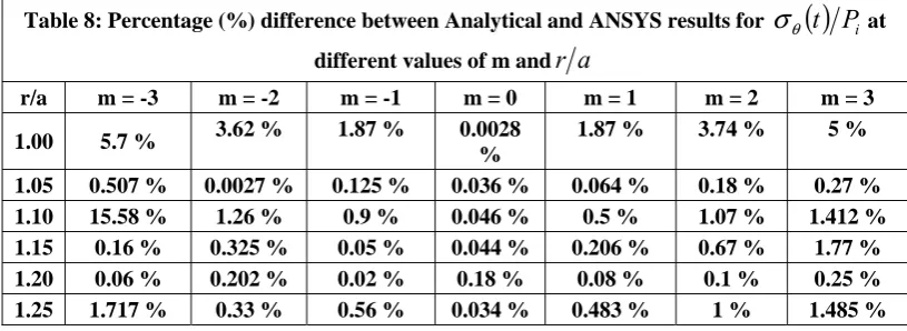
Table 8: Percentage (%) difference between Analytical and ANSYS results for

σ

_θ

( )

t

P

_i at different values of m and

r

a

r/a m = -3 m = -2 m = -1 m = 0 m = 1 m = 2 m = 3

1.00 5.7 % 3.62 % 1.87 % 0.0028

%

1.87 % 3.74 % 5 %

1.05 0.507 % 0.0027 % 0.125 % 0.036 % 0.064 % 0.18 % 0.27 %

1.10 15.58 % 1.26 % 0.9 % 0.046 % 0.5 % 1.07 % 1.412 %

1.15 0.16 % 0.325 % 0.05 % 0.044 % 0.206 % 0.67 % 1.77 %

1.20 0.06 % 0.202 % 0.02 % 0.18 % 0.08 % 0.1 % 0.25 %

1.25 1.717 % 0.33 % 0.56 % 0.034 % 0.483 % 1 % 1.485 %

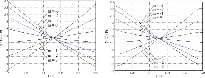
as well as with the values of the Analytical and ANSYS results in Table 7, the graphical plots of Tangential stress for thermal loading based on Analytical results and ANSYS results are shown in Fig. 11and 12, respectively.

Fig. 11: Tangential stress for thermal loading [Analytical results] Fig. 12: Tangential stress for thermal loading [ANSYS results]

4.3.2. Tangential stress for mechanical loading: Analytical vs. ANSYS and Percentage (%) difference between Analytical and ANSYS results

σ

_θ

( )

m

P

r

a

r/a

m = -3 [Analytical

]

m = -3 [ANSYS]

m = -2 [Analytical

]

m = -2 [ANSYS]

m = -1 [Analytical

]

m = -1 [ANSYS]

m = 0 [Analytical

]

m = 0 [ANSYS]

1.00 2.9397 2.87195 2.6333 2.5921 2.3445 2.3259 2.0738 2.074

1.05 2.338 2.3352 2.2062 2.2044 2.0713 2.0704 1.9343 1.9343

1.10 1.89062 1.88235 1.875 1.8703 1.851 1.8487 1.819 1.8191

1.15 1.5536 1.5484 1.61493 1.6112 1.6716 1.6696 1.723 1.7229

1.20 1.29611 1.2964 1.408265 1.4084 1.52383 1.52385 1.6421 1.64205

1.25 1.097 1.11555 1.24223 1.2562 1.40107 1.4089 1.5738 1.5737

Table 9: continued……of

σ

_θ

( )

m

P

r

a

r/a m = 1

[Analytical]

m = 1 [ANSYS]

m = 2 [Analytical]

m = 2 [ANSYS]

m = 3 [Analytical]

m = 3 [ANSYS] 1.00 1.82132 1.83695 1.58717 1.6151 1.3711805 1.4086

1.05 1.7963 1.7972 1.6585 1.6602 1.5219762 1.52445

1.10 1.7791 1.78165 1.731833 1.73685 1.67772 1.68515

1.15 1.7682 1.77045 1.80689 1.8116 1.83857 1.8459

1.20 1.7623 1.7622 1.88344 1.88335 2.00465 2.0046

(12)

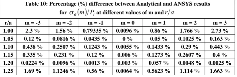
and the correspondingpercentage (%) difference between Analytical and ANSYS results are furnished in Table 10,

σ

_θ

( )

m

P

r

a

r/a m = -3 m = -2 m = -1 m = 0 m = 1 m = 2 m = 3

1.00 2.3 % 1.56 % 0.79335 % 0.0096 % 0.86 % 1.766 % 2.73 %

1.05 0.12 % 0.0816 % 0.0435 % 0 % 0.05 % 0.1025 % 0.163 %

1.10 0.438 % 0.2507 % 0.1243 % 0.0055 % 0.1433 % 0.29 % 0.443 %

1.15 0.335 % 0.231 % 0.12 % 0.006 % 0.1273 % 0.2607 % 0.4 %

1.20 0.0224 % 0.0096 % 0.0013 % 0.003 % 0.057 % 0.0048 % 0.0025 %

1.25 1.69 % 1.1246 % 0.56 % 0.0064 % 0.5623 % 1.114 % 1.663 %

as well as with the values of the Analytical and ANSYS results in Table 9, the graphical plots of Tangential stress for mechanical loading based on Analytical results and ANSYS results are shown in Fig. 13and 14, respectively.

Fig. 13: Tangential stress for mechanical loading [Analytical results] Fig. 14: Tangential stress for mechanical loading [ANSYS results]

4.3.3. Tangential stress for thermo-mechanical loadings: Analytical vs. ANSYS and Percentage (%) difference between Analytical and ANSYS results

σ

_θ

( )

r

P

r

a

r/a m = -3

[Analytical]

m = -3 [ANSYS]

m = -2 [Analytical]

m = -2 [ANSYS]

m = -1 [Analytical]

m = -1 [ANSYS]

m = 0 [Analytical]

m = 0 [ANSYS]

1.00 2.27606 2.24615 2.20563 2.17995 2.0678 2.0544 1.895 1.8951

1.05 2.0835 2.08225 2.0201 2.01835 1.9354 1.9347 1.836 1.83605

1.10 1.88074 1.8754 1.8518 1.84735 1.82243 1.82035 1.79036 1.7905

1.15 1.68683 1.68185 1.701 1.697 1.72513 1.7232 1.75502 1.7551

1.20 1.510 1.5104 1.567 1.5668 1.6406 1.64055 1.72768 1.72765

(13)

Table 11: continued……… of

σ

_θ

( )

r

P

r

a

r/a m = 1

[Analytical]

m = 1 [ANSYS]

m = 2 [Analytical]

m = 2 [ANSYS]

m = 3 [Analytical]

m = 3 [ANSYS]

1.00 1.7056 1.71905 1.5123 1.5374 1.32271 1.3571

1.05 1.725654 1.7265 1.60804 1.60965 1.48611 1.4885

1.10 1.753 1.75545 1.70933 1.7141 1.659 1.66615

1.15 1.78635 1.7886 1.81617 1.8208 1.84233 1.84955

1.20 1.82465 1.8246 1.92863 1.9286 2.037151 2.0372

1.25 1.86712 1.8567 2.046823 2.0241 2.2446 2.2074

Table 12,

σ

_θ

( )

r

P

r

a

r/a m = -3 m = -2 m = -1 m = 0 m = 1 m = 2 m = 3

1.00 1.32 % 1.164 % 0.65 % 0.0053 % 0.79 % 1.66 % 2.6 %

1.05 0.06 % 0.087 % 0.036 % 0.003 % 0.049 % 0.1 % 0.161 %

1.10 0.284 % 0.24 % 0.114 % 0.008 % 0.14 % 0.28 % 0.431 %

1.15 0.3 % 0.235 % 0.112 % 0.0046 % 0.126 % 0.255 % 0.392 %

1.20 0.027 % 0.013 % 0.003 % 0.002 % 0.003 % 0.0016 % 0.0024 %

1.25 1.7 % 1.105 % 0.56 % 0.0017 % 0.56 % 1.11 % 1.66 %

as well as with the values of the Analytical and ANSYS results in Table 11, the graphical plots of Tangential stress for thermo-mechanical loadings based on Analytical results and ANSYS results are shown in Fig. 15and 16, respectively.

Fig. 15: Tangential stress for thermo-mechanical loadings [Analytical] Fig. 16: Tangential stress for thermo-mechanical loadings [ANSYS]

It is observed that the percentage (%) differences between Analytical and FEA [ANSYS] results, of tangential stresses,

σ

_θ

( )

t

, for thermal loading (Table 8), 29 nos, out of the 42 nos, of percentage (%) difference are well below of 1 %, 08 nos, exceed 1 %, are well below of 2 % and the rest 05 nos exceed 3 %,

σ

_θ

( )

m

, for mechanical loading (Table 10), 34 nos, out of the 42 nos, of percentage (%) difference are well below of 1 %, 06 nos, exceed 1 %, are well below of 2 %, and the rest 02 nos, exceed 2 %, are well below of 3 %, and

( )

r

θ

(14)

4.4. Equivalent stress

4.4.1. Equivalent stresses:By Analytical method

The analytical results of the equivalent stress are obtained by

σ

_eq

=

2 (

σ

_θ

−

σ

_r

)

.

Table 13: Analytical results of

σ

_eq at different values of m and

r

a

[By Analytical method]

r/a m = -3 m = -2 m = -1 m = 0 m = 1 m = 2 m = 3 m = 4 m = 5

1.00 926.609 906.689 867.708 818.794 765.26 710.585 656.96 605.74746 557.73 1.05 788.469 772.427 751.384 726.822 699.536 670.343 639.953 608.9875 577.9544

1.10 663.62 658.358 654.144 649.95 644.792 638.166 629.83 619.7261 607.9054

1.15 554.685 561.577 572.184 585.111 598.977 612.815 625.906 637.743 647.94905 1.20 461.487 479.446 502.585 529.966 560.50 593.322 627.697 663.003 698.68314 1.25 382.647 409.66 443.078 482.705 528.101 578.928 634.87 695.6446 760.9563

4.4.2. Equivalent stresses:By Finite element method

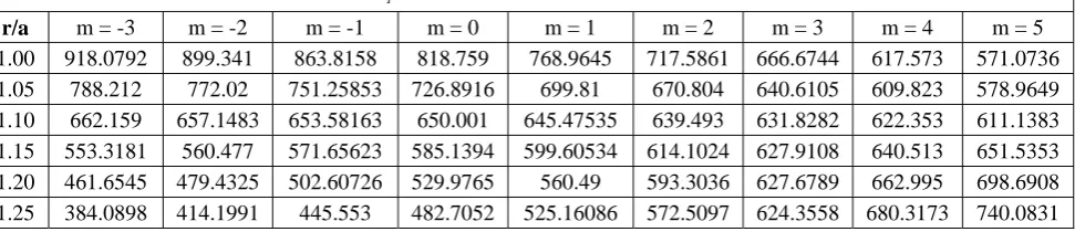
Table 14: ANSYS results of

σ

_eq at different values of m and

r

a

[By Finite element method]

r/a m = -3 m = -2 m = -1 m = 0 m = 1 m = 2 m = 3 m = 4 m = 5

1.00 918.0792 899.341 863.8158 818.759 768.9645 717.5861 666.6744 617.573 571.0736

1.05 788.212 772.02 751.25853 726.8916 699.81 670.804 640.6105 609.823 578.9649 1.10 662.159 657.1483 653.58163 650.001 645.47535 639.493 631.8282 622.353 611.1383 1.15 553.3181 560.477 571.65623 585.1394 599.60534 614.1024 627.9108 640.513 651.5353 1.20 461.6545 479.4325 502.60726 529.9765 560.49 593.3036 627.6789 662.995 698.6908 1.25 384.0898 414.1991 445.553 482.7052 525.16086 572.5097 624.3558 680.3173 740.0831

4.4.3. Percentage (%) differencebetween Analytical and ANSYS results of Equivalent stress for thermo-mechanical loadings

Based on the resultsof Tables 13 and 14, the correspondingpercentage (%) difference between Analytical and ANSYS results are furnished in Table 15,

Table 15: Percentage (%) difference between Analytical and FEA [ANSYS] results for

σ

_eq

r/a m = -3 m = -2 m = -1 m = 0 m = 1 m = 2 m = 3 m = 4 m = 5

1.00 0.92 % 0.81 % 0.45 % 0.004 % 0.5 % 0.985

% 1.479 % 1.952 % 2.392 %

1.05 0. 033 % 0.053 % 0.017 % 0.01 % 0.04 %

0.069

% 0.103 % 0.137 % 0.175 %

1.10 0.22 % 0.184 % 0.46 % 0.008 % 0.106 %

0.208

% 0.317 % 0.424 % 0.532 %

1.15 0.25 % 0.196 % 0.092 % 0.005 % 0.105

% 0.21 % 0.32 % 0.434 % 0.553 %

1.20 0.036 % 0.003 % 0.004 % 0.002 % 0.002 %

0.003

% 0.003 % 0.001 % 0.001 %

1.25 0.38 % 1.108 % 0.56 % 0.001 % 0.56 %

1.036

% 1.656 % 2.203 % 2.743 %

4.4.4. Graphical plots of Equivalent stress for thermo-mechanical loadings based on Analytical and FEA results

(15)

Fig.17: Equivalent stress for thermo-mechanical loadings [Analytical] Fig 18: Equivalent stress for thermo-mechanical loadings [ANSYS]

It is observed that the percentage (%) differences between Analytical and FEA [ANSYS] results, of equivalent stress,

σ

_eq,for thermo-mechanical loadings (Table 15) , 46 nos, out of the 54 nos, of percentage (%) difference are well below of 1 %, 05 nos, exceed 1 %, are below of 2 %, and the rest 03 nos, exceed 2 %, are well below of 3 %.Table 15 clearly shows the results of the Analytical (Theoretical) Analysis with those of the Finite Element Analysis (FEA) are in very good agreement.

5. Conclusions

The following points are concluded based on the analysis:

(1) The finite element analysis (FEA) steps are implemented using ANSYS Parametric Design Language (APDL).

(2) The final equations are already validated by [Nayak et al. (2011)] with substituting zeroes for the indices

m1, m2, m3 and in turn, obtaining the expressions for an isotropic and homogenous sphere those are same as

specified in [Chakrabarty, (1998); Noda et al. (2003)]. Again, they also validated the final equations by taking a numerical example (problem) and for the comparative study with the finite element analysis (FEA), the same problem is taken.

(3) The percentage (%) differences between Analytical and FEA [ANSYS] results, of radial stresses, for thermal loading , all the 42-nos of percentage (%) difference are well below of 1 %, for mechanical loading , all the nos of percentage (%) difference are well below of 1 %, and for thermo-mechanical loadings, all the 42-nos of percentage (%) difference are also well below of 1 %. It clearly shows that the results of the Analytical (Theoretical) Analysis with those of the Finite Element Analysis (FEA) are in very good agreement.

(4) The percentage (%) differences between Analytical and FEA [ANSYS] results, of tangential stresses, for thermal loading, 29 nos, out of the 42 nos, of percentage (%) difference are well below of 1 %, 08 nos, exceed 1 %, are well below of 2 % and the rest 05 nos exceed 3 %, for mechanical loading, 34 nos, out of the 42 nos, of percentage (%) difference are well below of 1 %, 06 nos, exceed 1 %, are well below of 2 %, and the rest 02 nos, exceed 2 %, are well below of 3 %, and for thermo-mechanical loadings, 34 nos, out of the 42 nos, of percentage (%) difference are also well below of 1 % and the rest 08 nos, exceed 1 %, are well below of 2 %. It clearly shows that the results of the Analytical (Theoretical) Analysis with those of the Finite Element Analysis (FEA) are in very good agreement.

(16)

References

[1] Alisafaei F., Ansari R. (2012): Dynamic analysis of heterogeneous pressure vessels subjected to thermo-mechanical loads. Pressure vessel technology ASME, vol. 134, pp. 1-10.

[2] Chakrabarty, J. (1998): Theory of Plasticity. McGraw Hill, New York.

[3] Chen, Y. Z,; Lin, X. Y. (2008): Elastic analysis for thick cylinders and spherical pressure vessels made of functionally graded materials.Computational Materials Science, 44, pp. 581–587.

[4] Esteban S. L., Bartolome J. F., Pecharroman C., Moya J. S. (2002): Zirconia/stainless-steel continuous functionally graded material. European Ceramic Society, vol. 22, pp. 2799-2804.

[5] Jabbari M., Bahtui A., Eslami M. R. (2009): Axisymmetric mechanical and thermal stresses in thick short length FGM cylinders. Pressure vessels and piping, vol.86, pp.296-306.

[6] Jabbari M., Meshkini M., Eslami M. R. (2012) : Nonaxisymmetric mechanical and thermal stresses in FGPPM hollow cylinder. Pressure vessel technology ASME, vol. 134, pp. 1-25.

[7] Jabbari M., Meshkini M., Eslami M. R. ( 2015):Mechanical and thermal stresses in FGPPM hollow cylinder due to radially symmetric loads.Pressure vessel technology ASME, vol. 138 (1), 011207(9 pages).

[8] Jabbari M., Mousavi S. M., Kiani M. A. (2016): Solution for equation of two- dimensional transient heat conduction in functionally graded material hollow sphere with piezoelectric internal and external layers. Pressure vessel technology ASME, vol. 139(1), 011201(6 pages).

[9] Liew, K. M.; Kitipornchai, S.; Zhang, X. Z.; Lim,C. W. (2003): Analysis of the thermal stress behaviour of functionally graded hollow circular cylinders.Solids and Structures, 40, pp. 2355–80.

[10] Nayak P., Mondal S. C., Nandi A.(2011): Stress, strain and displacement of a functionally graded thick spherical vessel. Engineering science and technology, vol 3(4), pp. 2659-2671.

[11] Nejad M. Z., Abedi M., Lotfian M. H., Ghannad M. (2011): Exact and numerical solutions for stresses in pressurized FGM solid sphere with parabolic varying properties. American journal of scientific research, vol. 32, pp. 82-89.

[12] Noda N., Hetnarski R. B., Tanigawa Y. (2003): Thermal Stresses. Taylor and Francis, New York. [13] Ozisik, M. N. (1985): Heat Transfer. McGraw Hill, New York.

[14] Peng, X. L.; Li, X. F. (2010): Thermo-elastic analysis of a cylindrical vessel of functionally graded materials. Pressure vessels and piping, 87, pp. 203-210.

[15] Poultangari R., Jabbari M., Eslami M.R. (2008): Functionally graded hollow spheres under non-axisymmetric thermo-mechanical loads. Pressure vessels and piping, vol.85, pp. 295–305.

[16] Sadeghian M., Toussi H. E. (2010): Axisymmetric yielding of functionally graded spherical vessel under thermo-mechanical loading. Computational materials science.

[17] Santos H., Mota Soares C. M., Mota Soares C. A., Reddy J.N. (2008): A semi-analytical finite element model for the analysis of cylindrical shells made of functionally graded materials under thermal shock. Composite structures, vol. 86, pp. 10–21.

[18] Shao, Z. S. (2005): Mechanical and thermal stresses of a functionally graded hollow circular cylinder with finite length. Pressure vessel and piping, 82, pp.155-163.

[19] Shao, Z. S.; Ma, G. W. (2008): Thermo-mechanical stresses in functionally graded circular hollow cylinder with linearly increasing boundary temperature.Composite Structures, 83, pp.259–265.

[20] Shariyat M. (2009): A nonlinear Hermitian transfinite element method for transient behavior analysis of hollow functionally graded cylinders with temperature-dependent materials under thermo-mechanical loads. Pressure vessels and piping, vol. 86, pp.280–289. [21] Tutuncu N, Ozturk M. (2001): Exact solutions for stresses in functionally graded pressure vessels. Composites, part B, 32, pp.

683-686.

[22] You, L. H.; Zhang, J. J.; You, X. Y. (2005): Elastic analysis of internally pressurized thick-walled spherical pressure vessels of functionally graded materials. Pressure vessel and piping, 82, pp.347-354.

Appendix A

Various constants:

A.1

(

)

(

1 2

) ( )

1

2 2 1 1 0 2 1 1 ln − − − − − ₊ ₊ − − = ba b h a h k T T

Z ,

(

)

(

1 2

)

(

1

)

2 2 1 1 0 1 2 1 1 2 1 2 1 2 2 1 1 1 1 0 2 1 2 ln ] ln ln [ − − − − − − − − − − − − − + + + − + = ba b h a h k b T a T b h T a h T k T T Z

(

)

(

)

(

1 2

)

( 1) ( 1)

2 2 1 1 0 3 2 1

3 ₃ ₃

1 − − + − − + − + − − +

+

−

= _m _k _h _a _h _b _a m _b m

T T

Z and

(

)

(

)

( ) ( )

(

)

(

1 2

)

( 1) ( 1)

2 2 1 1 0 3 1 1 2 1 1 1 2 1 2 1 2 2 1 1 1 1 0 3 2 1 4 3 3 3 3 1 ] 1 [ + − + − − − − − + − − + − − − − − − − − − + + + − + + +

= _m m _m m

b a b h a h k m b T a T b h T a h T k m T T Z

(17)

A.2

(

ν

)(

ν

)

ν λ 2 1

1+ −

= E and

₍

₎

ν + = 1 2 E G

A.3

(

)

_,

(

)

_,

1 1 2 , 2 , 1 1 2 1 0 1 1 1

1 M Z m m

m P R m P Q

P  = +

     − − + = + =       + − = α ν ν ν ν ν

N₁ =α₀

{

Z₁ +Z₂

(

m₁ +m₂

)

}

,M₂ =Z₃α₀

(

m₁ +m₂ −m₃ −1

)

,and .N₂ =Z₄α₀

(

m₁ +m₂

)

{

}(

)

[

Pm Q m R

]

M Y + + + = 1 2 2 1

1 ,

[

( )( )

]

[

( )

]

( )( )

[

]

2

2 2 2 1 2 2 1 2 1 1 2 1 R m Q Pm Q m P M R m Q Pm N Y + + + + + − + + + =

(

)

{

}(

)

[

P m m Q m m R

]

M Y + − + − − = 3 2 3 2 2 3 1 and ( )( )

[Pm Q m R]

N Y + + + = 1 2 2 2 4

(

1 ν

)(

1 2ν

)

0

− +

= E

D ,

(

)

{

(

) (

)

} (

)

(

) (

)

{

} (

)

_      + − − + + + + − − + + + − = ₊ + r r Z m Y r Z m Y Y

D _m _m

m m ln 1 1 1 1 1 1 1 2 1 2 1 0 1 2 1 0 2 2 2 1 α ν ν ν α ν ν ν ν δ

and

{

(

) (

)

} (

)

(

)(

)

{

} (

)

_      + − − − + + + − − + + = Δ ₊ ₋ ₋ + 1 0 3 3 2 3 01 4 2 4 3 2 1 2 1 1 1 2 1 1 1 m m m m m r Z m m Y r Z m Y D α ν ν ν α ν ν ν

[

2

(

1

)

]

1,

1 1

1

1+ −

− +

= m s

a D ν ν s a

β

[

2

(

1

)

]

1,

2 2

2

1+ −

− +

= m s

a D ν ν s a

β

[

(

)

]

1

1 1

1

2 + − + −

= m s

b D ν ν s b

β and

[

(

)

]

1

2 2

2 1

1

2 + − + −

= m s

b D ν ν s b

β

(

)

(

)

1 2 2 1 2 2 1 b a b a a i b b o

a p p

X β β β β δ β δ β − + − +

= and

(

)

(

)

1 2 2 1 1 1 2 b a b a b o a a i

b p p

X β β β β δ β δ β − + − + =

(

)

(

)

1 2 2 1 2 2 3 b a b a a i b b o

a p p

X β β β β β β − Δ + − Δ +

= and

(

)

(

)

1 2 2 1 1 1 4 b a b a b o a a i

b p p

X β β β β β β − Δ + − Δ + =