This may be the author’s version of a work that was submitted/accepted for publication in the following source:
Jones, Andrew, Ovenden, Jennifer, &Wang, You-Gan (2016)
Improved confidence intervals for the linkage disequilibrium method for estimating effective population size.
Heredity,117(4), pp. 217-223.
This file was downloaded from: https://eprints.qut.edu.au/104248/
c
Consult author(s) regarding copyright matters
This work is covered by copyright. Unless the document is being made available under a Creative Commons Licence, you must assume that re-use is limited to personal use and that permission from the copyright owner must be obtained for all other uses. If the docu-ment is available under a Creative Commons License (or other specified license) then refer to the Licence for details of permitted re-use. It is a condition of access that users recog-nise and abide by the legal requirements associated with these rights. If you believe that this work infringes copyright please provide details by email to qut.copyright@qut.edu.au
Notice:Please note that this document may not be the Version of Record (i.e. published version) of the work. Author manuscript versions (as Sub-mitted for peer review or as Accepted for publication after peer review) can be identified by an absence of publisher branding and/or typeset appear-ance. If there is any doubt, please refer to the published source.
Improved Confidence Intervals for the Linkage Disequilibrium
1
Method for Estimating Effective Population Size
2
A. T. Jones*, J. R. Ovenden†, Y-G Wang*,+ 3
*Centre for Applications in Natural Resource Mathematics, School of Mathematics and 4
Physics, The University of Queensland, St Lucia, 4072, Queensland, Australia. 5
† Molecular Fisheries Laboratory, School of Biomedical Sciences, University of Queensland, 6
St Lucia, 4072, Queensland, Australia. 7
+Corresponding Author: Professor You-Gan Wang, School of Mathematical Sciences
8
Science and Engineering Faculty, Queensland University of Technology, Brisbane 4001, 9
Australia, email: you-gan.wang@qut.edu.au 10
11
Running Title: Improved Confidence Intervals for 𝑁𝑁𝑒𝑒
12
Word Count: 4377 13
14
15
Abstract
16
The linkage disequilibrium method is currently the most widely used single sample 17
estimator of genetic effective population size. Commonly used software packages come 18
with two options, referred to as the parametric and jackknife methods, for computing the 19
associated confidence intervals. However little is known on the coverage performance of 20
these methods, and the published data suggests there may be some room for improvement. 21
Here we propose two new methods for generating confidence intervals and compare them 22
with the two in current use through a simulation study. The new CI methods tend to be 23
conservative but outperform the existing methods for generating confidence intervals 24
under certain circumstances, such as those that may be encountered when making 25
estimates using large numbers of SNPs. 26
Keywords: linkage disequilibrium, effective population size, confidence intervals 27
Introduction
28
Effective population size (𝑁𝑁𝑒𝑒) is an important parameter of interest to the study of
29
evolutionary biology as well as for monitoring species of conservation concern. The linkage 30
disequilibrium method is the most commonly used genetic estimator of contemporary 𝑁𝑁𝑒𝑒.
31
Its popularity stems from its ability to make powerful estimates from single samples, 32
whereas the so-called temporal methods require two or more samples from a population 33
separated in time. The linkage disequilibrium method is also easily accessible through 34
several software packages namely the programs LDNe(Waples and Do, 2008) and 35
NeEstimator 2.0 (Do et al, 2014) . 36
There are a number of studies investigating the effectiveness of the linkage disequilibrium 37
method (Luikart et al, 2010; Waples, 2005; Waples and Do, 2010; Waples and Gaggiotti, 38
2006). However there is little work published with regard to the performance of the 39
associated confidence intervals. From the statistical perspective 𝑁𝑁�𝑒𝑒, like any other
40
estimator, is a random variable with a distribution. Unfortunately, the distribution of 𝑁𝑁�𝑒𝑒 is
41
not easy to characterize, and therefore, the exact confidence intervals are not available. The 42
current practice is based on a scaled chi-square distribution. However the corresponding 43
number of degrees of freedom is not well defined due to the intrinsic correlations between 44
individual estimates of linkage disequilibrium , which are combined to estimate 𝑁𝑁𝑒𝑒.
45
For any method of generating confidence intervals at any significance level, the true value 46
of an estimated parameter must inevitably fall in some proportion of confidence intervals. 47
Ideally, for accurate confidence intervals generated at a significance level of α , this 48
proportion will be (1 − 𝛼𝛼), in the long run. That is to say, if a researcher were to generate 49
many 95% confidence intervals, they ought to be able to expect that 95% of the time the 50
true value of the parameter they are estimating will lie in its interval. If the intervals are set 51
too narrowly then the true values will not lie in the confidence intervals as often as they 52
should and the certainty of the estimates will be overstated. This is referred to as being 53
anti-conservative. The proportion of the time that confidence intervals do actually contain 54
the true value of the estimated parameter is commonly referred to as the coverage 55
probability. Conversely, if the coverage probability is too high the confidence interval is 56
said to be conservative. 57
If confidence intervals are to be valid and useful, the coverage probability ought to be the 58
same as the nominal value for that interval (i.e. 0.95 for a 95% confidence interval). This 59
ought to hold for all values of 𝛼𝛼, not just the standard 0.05 / 95% case. It should also hold 60
for all values of any other parameters that may affect the estimates. In the case of effective 61
population size these include population size (N), number of Loci (L), number of alleles at 62
each locus (K), and sample size (S). 63
A direct method to determine confidence intervals for linkage disequilibrium estimates of 64
population size was not provided in the original formulation of the method (Hill, 1981). 65
The LDNE (Waples and Do, 2008) and NeEstimator 2.0 (Do et al, 2014) software packages 66
provide two methods for generating confidence intervals. The first, referred to as the 67
‘parametric method’ (Waples, 2006) is based on a technique used for confidence intervals 68
for the temporal method (Waples, 1989). It takes the distribution for r�2⁄𝔼𝔼[r�2] to be a 𝜒𝜒2
69
distribution with the degrees of freedom being equal to the total number of ‘independent 70
comparisons’ used in the estimation. 71
The second is a ‘jackknife’ based correction to this method (Waples and Do, 2008). An 72
approximate relationship using a re-estimated parameter is used to adjust the degrees of 73
freedom in the 𝜒𝜒2 distribution in the confidence interval. The rationale behind this
74
technique is that the true value for the degrees of freedom in the 𝜒𝜒2 distribution used in
75
confidence intervals is less than the total number of comparisons, because the comparisons 76
are not all independent . As such, we expect that the performance of the ‘parametric 77
method’ and perhaps also this ‘jackknife’ based correction will decline as the total number 78
of comparisons grows. 79
However, strictly speaking, this method is not actually a jackknife technique as no 80
observations (individuals) are being removed only predictors (loci pairs). This is illustrated 81
by the fact no new calculations are needed for finding the new values, only a re-averaging 82
of existing values. Whereas, if individuals were removed one at a time instead, the linkage 83
would have to be recalculated for each loci pair every time. In addition, the variance is not 84
estimated in the standard jackknife fashion. Henceforth we refer to this method as the 85
‘pseudo-jackknife’. While the pseudo-jackknife requires more computation time than the 86
parametric method, a full jackknife based on individuals would require yet more. 87
Published confidence interval results for the parametric and pseudo-jackknife methods 88
(Waples and Do, 2008) show it is possible for the confidence intervals to be insufficiently 89
conservative and contain fewer than the nominal proportion of values. For instance, a 90
nominal 95 % interval may on average only contain the true value 80 % of the time. These 91
results suggest that there is room for improvement in the performance of these confidence 92
intervals. 93
Two variations of the application of the jackknife are proposed and tested in this paper as 94
possible improvements on the existing techniques. To test a confidence interval method it 95
is necessary to know the true value of the parameter being estimated. This means that for 96
genetic estimates of 𝑁𝑁𝑒𝑒, simulated populations are required. The simplest method to
97
empirically test the coverage probability for a given method of generating confidence 98
intervals is to simulate a large number of replicate populations with known 𝑁𝑁𝑒𝑒, make
99
estimates of this 𝑁𝑁𝑒𝑒and produce the associated confidence intervals, and then see how
100
often the (known) true value falls inside these intervals. The proportion of intervals 101
containing the true value will estimate the coverage probability for that method. 102
There is reason to believe that current methods for generating confidence intervals for 103
estimates of 𝑁𝑁𝑒𝑒using the linkage disequilibrium method may be suboptimal in at least
104
some cases. Two newer methods are proposed that may outperform the older methods and 105
all were tested on wide range of simulated population scenarios. The performance of all 106
four methods in terms of coverage probability is examined, with the objective of 107
recommending under which circumstances, if any, each of the methods should be used. 108
Materials and Methods
109
Effective population size estimation
110The original, uncorrected, formula for 𝑁𝑁�𝑒𝑒(Hill, 1981) is given by
111
𝑁𝑁^ =𝑒𝑒 3(𝑟𝑟^2− 1/𝑆𝑆) ,1 (1)
where S is the samples size, and 𝑟𝑟^2 is a measure of the association between alleles at
112
different loci. However, this formula was corrected based on empirical work (Waples, 113
2006; Waples and Do, 2008), and replaced in practice by 114
115
𝑁𝑁^ = 1/3�1/9 − 2.76𝑟𝑟^𝑒𝑒 2
2(𝑟𝑟^2− 1/𝑆𝑆) , (2)
for the case of random mating with a sample size greater than 30. Similar formulas for 116
other cases were also given. 117
The linkage disequilibrium method was originally derived for the case of one pair of loci 118
with two alleles per locus (Hill, 1981) . Where there are more than two alleles at a locus, 119
the alleles must be split up and the pairwise estimates from each allele pairs (one from 120
each locus) must be averaged within that loci pair, before the average across loci pairs is 121
taken. Each value of 𝑟𝑟^2, is estimated in practice using the Burrows’ Composite Method
122
(Cockerham and Weir, 1977), which is robust to deviations from pure random mating and 123
unbiased when corrected by a factor of 𝑆𝑆 (𝑆𝑆 − 1)⁄ (Weir, 1979). The full formula is 124
𝑟𝑟^2 = [𝑆𝑆 (𝑆𝑆 − 1⁄ )∆]2
[𝑝𝑝(1 − 𝑝𝑝)(𝑝𝑝𝐴𝐴− 𝑝𝑝2)][𝑞𝑞(1 − 𝑞𝑞)(𝑝𝑝𝐴𝐴− 𝑞𝑞2)] , (3)
where ∆ is the original Burrows coefficient, S is the sample size, 𝑝𝑝(𝑞𝑞) is the observed 125
frequency of the allele at the first (second) locus, and 𝑝𝑝𝐴𝐴 and 𝑝𝑝𝐵𝐵 are the frequencies of
126
homozygotes of the alleles at their respective loci. 127
In all cases we examined, 𝑟𝑟^2 is averaged across loci pairs according to the methodology
128
used in the NeEstimator 2.0 (Do et al, 2014) software as based on earlier work (Waples 129
and Do, 2008) . This global average is referred to as 𝑟𝑟2. We do not examine the case of 130
missing data and thus did not have recourse to the weighting techniques which have been 131
developed for this (Peel et al, 2013) . 132
This averaging of many estimates gives rise to the idea of a total number of comparisons, J, 133
used in making an estimate. A single ‘comparison’ is the estimate of 𝑟𝑟^2 produced by a single
134
pair of alleles, one each from a pair of loci. If there are 𝐿𝐿 loci and each locus 𝑖𝑖 has 𝐾𝐾𝑖𝑖 alleles
135
then the total number of nominally independent comparisons according to this method is 136
𝐽𝐽 = � (
𝑖𝑖,𝑗𝑗∈𝐿𝐿,𝑖𝑖<𝑗𝑗
𝐾𝐾𝑖𝑖− 1)(𝐾𝐾𝑗𝑗− 1). (4)
For example, with 10 loci and 15 alleles per loci, 𝐽𝐽 = 8820. This is a fairly typical result in 137
practice. 138
A complication in the calculation of 𝑟𝑟^2is that rare alleles are known to cause bias. That is,
139
alleles with low observed frequencies, tend to produce upwardly biased estimates (Waples, 140
2006; Waples and Do, 2010). The standard method to deal with this problem is to discard 141
all values of 𝑟𝑟^2 produced from allele pairs where one or both members of the pair have an
142
observed frequency (proportion) below a given cut-off. This cut-off is referred to as 𝑝𝑝𝑐𝑐𝑐𝑐𝑖𝑖𝑐𝑐
143
and is typically in the range [0 , 0.1]. This impacts the confidence intervals for 𝑁𝑁�𝑒𝑒 in several
144
ways. While removing low frequency alleles reduces bias, it also increases the variance of 145
the estimate(Waples and Do, 2010). Removing alleles also decreases the number of 146
comparisons used in the calculation. The results from two values of 𝑝𝑝𝑐𝑐𝑐𝑐𝑖𝑖𝑐𝑐 are reported for
147
this study, 0, that is with no alleles removed at all, and 0.05, a moderately high value. 148
Simulated Populations
149The software package SimuPOP(Peng and Kimmel, 2005) was used to simulate 150
standardized populations with known effective population sizes for the testing of the 151
various confidence interval methods. The populations were individual based, forward time 152
simulations with discrete generations and unlinked loci. 153
It is known that in such simulations, the realized 𝑁𝑁𝑒𝑒 will not match the nominal value but
154
will vary somewhat between simulated generations (Waples and Faulkner, 2009). As such, 155
for the purposes of determining if a confidence interval contained the true value or not, the 156
demographic effective population size was calculated for each case. The appropriate 157
formula (Crow and Denniston, 1988) is 158
𝑁𝑁𝑒𝑒 = 𝑘𝑘𝑁𝑁 − 2
𝑘𝑘 − 1 + 𝑉𝑉𝑘𝑘/𝑘𝑘+ 0.5 (5)
for the case of separate sexes. N is the population size, 𝑘𝑘 is the mean number of offspring 159
per individual and 𝑉𝑉𝑘𝑘 is the variance of the same quantity. Fortunately, all of these
160
parameters are easily retrieved from the simulation data. The linkage disequilibrium 161
method estimates the population of the parental generation of the sampled generation. 162
However the linkage ‘signal’ from prior generations also persists, declining by a factor of 2 163
every generation. The true value for 𝑁𝑁𝑒𝑒 , to be compared with its estimates, is taken to be
164
the harmonic mean of the demographic 𝑁𝑁𝑒𝑒 for the 4 generations prior to the sampled
165
generation, weighted by their relative contributions which halve each generation further 166
back in time (i.e. 0.5, 0.25, 0.125, 0.0625). 167
The simulations encompassed a wide variety of scenarios with varying sample sizes (S), 168
population sizes (N), number of alleles per locus (K), number of loci (L), and allele 169
frequency distributions, number of burn in generations (g). Table 1 summarizes these 170
scenarios and also includes the associated value of the total number of comparisons, J, 171
which is believed to be the main factor in the decline in confidence interval performance. It 172
reports them in terms of, Jmax is the total number of comparisons if no alleles go to
173
extinction during the simulation and no rare alleles are discarded, as well as a figure for 174
how many comparisons are actually used when a 𝑝𝑝𝑐𝑐𝑐𝑐𝑖𝑖𝑐𝑐 of 0.05 is applied. This second
175
figure is an average across all of the replicate populations for that scenario. 176
Current Methods
177With all of the methods we initially find a confidence interval for 𝑟𝑟2. The upper and lower 178
bounds are then placed in either Equation 2 to produce the equivalent bounds for 𝑁𝑁𝑒𝑒. The
179
parametric method assumes the value 𝐽𝐽𝑟𝑟2 has a 𝜒𝜒2 distribution with 𝐽𝐽 degrees of freedom,
180
where 𝐽𝐽 is the total number of ‘independent comparisons’ used to calculate 𝑟𝑟2, as in 181
Equation 4. In the simplest case of a two loci with two alleles each r�2⁄𝔼𝔼[r�2] has an
182
approximately 𝜒𝜒2 distribution (Waples, 2006; Waples and Do, 2008) with a single degree of
183
freedom . The sum of these estimates 𝐽𝐽𝑟𝑟2 can be scaled to a 𝜒𝜒2 distribution with 𝐽𝐽 degrees
184
of freedom if all of the 𝑟𝑟^2 are independent. Thus a (1 − 𝛼𝛼) confidence interval for 𝑟𝑟2 is
185
� 𝑟𝑟
2𝐽𝐽
𝜒𝜒𝐽𝐽,21−𝛼𝛼/2, 𝑟𝑟 2𝐽𝐽
𝜒𝜒𝐽𝐽,2(1−𝛼𝛼)/2� .
The notation 𝜒𝜒𝐽𝐽,𝛼𝛼/22 indicates the (𝛼𝛼/2)𝑐𝑐ℎ percentile of 𝜒𝜒2 distribution with 𝐽𝐽 degrees of
186
freedom. As has been noted (Waples, 2006), this will overestimate the true degrees of 187
freedom as it does not account for potential correlations between the comparisons. It is 188
expected that this approximation will worsen as J increases (Do et al, 2014) . 189
The pseudo-jackknife builds on the parametric method but tries to account for the fact that 190
the pairs of alleles used to estimate 𝑟𝑟2are not actually independent of each other. Multiple 191
estimates within a pair of loci will obviously have correlations and even if all loci are 192
independently segregating, loci pairs that share a member will be correlated. It is possible 193
(Hill, 1981) to make an approximation 𝐽𝐽 ≈ 2/𝜙𝜙 where 𝜙𝜙 = 𝑉𝑉𝑉𝑉𝑟𝑟(𝑟𝑟2)/(𝑟𝑟2)2 is the
194
coefficient of variation. This approximation comes from derivation of the simple two locus 195
case with no covariance structure. This relationship is used (Waples, 2006) to re-196
approximate 𝐽𝐽 using a pseudo-jackknifed estimate of 𝜙𝜙 (Waples and Do, 2008). With 𝐿𝐿 loci 197
the total number of loci pairs is 𝐿𝐿(𝐿𝐿 − 1)/2 . Each pair is removed one at a time and 198
𝜙𝜙𝑖𝑖 = 𝑉𝑉𝑉𝑉𝑟𝑟(𝑟𝑟^−𝑖𝑖2)/(𝑟𝑟^−𝑖𝑖2)2 is computed in each case, 𝜙𝜙𝑖𝑖 being the coefficient of variation
199
calculated using 𝑟𝑟^−𝑖𝑖2, the estimate of 𝑟𝑟2 all but the 𝑖𝑖𝑐𝑐ℎ pair of loci. The sample variance is
200
used to estimate (𝑟𝑟^−𝑖𝑖2) , rather than the jackknife variance formula. These are then averaged
201
𝐽𝐽′ = 2/𝜙𝜙′ = 2 1
𝐶𝐶 � 𝜙𝜙𝑖𝑖
𝐶𝐶
𝑖𝑖=1
� = 2 𝐶𝐶 �1 𝑉𝑉𝑉𝑉𝑟𝑟(𝑟𝑟^−𝑖𝑖2) (𝑟𝑟^−𝑖𝑖2)2 𝐶𝐶
𝑖𝑖=1
� (6)
and the new estimate of 𝐽𝐽 is given by 𝐽𝐽′ = 2/𝜙𝜙′. The (1 − 𝛼𝛼) confidence interval for 𝑟𝑟2 is 202
then 203
� 𝑟𝑟2𝐽𝐽′ 𝜒𝜒𝐽𝐽2′,1−𝛼𝛼/2,
𝑟𝑟2𝐽𝐽′ 𝜒𝜒𝐽𝐽′,2(1−𝛼𝛼)/2� .
Owing to the idiosyncratic nature of the pseudo-jackknife procedure it may not correctly 204
account for the correlations between loci as expected. It is even the case that J’ is 205
sometimes higher than J, see Figure 3. 206
New Methods
207The limitations of the previous methods lead to directly to the application of a standard 208
jackknife technique(Efron and Gong, 1983). The linkage 𝑟𝑟−𝑖𝑖2 is 𝑟𝑟2 recalculated with the 𝑖𝑖𝑐𝑐ℎ
209
individual removed from the data set. The mean of these 𝑟𝑟−𝑖𝑖2 is then taken, that is,
210
𝑟𝑟̅(∙)2 = 1
𝑆𝑆 � 𝑟𝑟̅−𝑖𝑖2 𝑆𝑆
𝑖𝑖=1
(7)
Using a normal distribution for 𝑟𝑟2could be problematic as 𝑟𝑟2cannot take negative values. 211
One solution is to perform a Fisher Transformation on each of the 𝑟𝑟̅−𝑖𝑖2, that is, take
212
𝑧𝑧−𝑖𝑖 = tanh−1(𝑟𝑟̅
−𝑖𝑖2 ) (8)
and their mean to be 213
𝑧𝑧 = 1𝑆𝑆 �𝑧𝑧−𝑖𝑖
𝑆𝑆
𝑖𝑖=1
(9)
Then a confidence interval for 𝑧𝑧 based on the normal distribution can be constructed as 214
𝑧𝑧 ± Φ𝛼𝛼 2−1⁄ 𝑆𝑆𝑆𝑆� that is,
215
�𝑧𝑧 − Φ𝛼𝛼 2−1⁄ 𝑆𝑆𝑆𝑆� , 𝑧𝑧 + Φ𝛼𝛼 2−1⁄ 𝑆𝑆𝑆𝑆� �,
where Φ𝛼𝛼 2−1⁄ is the inverse standard normal function evaluated at (𝛼𝛼/2)Aandand, 𝑆𝑆𝑆𝑆�, the
216
jackknife standard error (Efron and Gong, 1983) is given by 217
𝑆𝑆𝑆𝑆� = �𝑆𝑆 − 1𝑆𝑆 �(𝑧𝑧−𝑖𝑖 − 𝑧𝑧)2 𝑆𝑆
𝑖𝑖=1
�
1 2⁄
(10)
The confidence interval can then be transformed back for 𝑟𝑟2as 218
�tanh�𝑧𝑧 − Φ𝛼𝛼 2−1⁄ 𝑆𝑆𝑆𝑆� � , tanh�𝑧𝑧 + Φ𝛼𝛼 2−1⁄ 𝑆𝑆𝑆𝑆� ��,
Computationally this is quite intensive compared with the previous method, however the 219
total time for a single estimate is still relatively short. 220
While the sample distribution of 𝑟𝑟2 remains largely unknown (Ethier and Griffiths, 1990;
221
Golding, 1984; Hudson, 2001; Schaid, 2004), there is some theoretical basis (Hill, 1981) 222
that distribution of is approximately 𝜒𝜒2 and using a normal distribution for the confidence
223
interval may be an inappropriate approximation. Another approach would be to use the 224
same relationship, 𝐽𝐽 ≈ 2/𝜙𝜙, but to use the jackknife estimate of the variance (𝑉𝑉𝑉𝑉𝑟𝑟� ) to 225
recalculate the degrees of freedom as 𝐽𝐽∗ and also using the jackknife mean 𝑟𝑟̅
(∙)2 in place of
226
𝑟𝑟2. This produces confidence intervals of the form 227
�𝑟𝑟̅(∙)2𝐽𝐽∗ 𝜒𝜒𝐽𝐽∗,𝛼𝛼
2
2 ,
𝑟𝑟̅(∙)2𝐽𝐽∗
𝜒𝜒𝐽𝐽∗,1−1−𝛼𝛼 2
2 � .
𝐽𝐽∗is calculated as
228
𝐽𝐽∗ = 2/𝜙𝜙∗= 2 𝑉𝑉𝑉𝑉𝑟𝑟�
�𝑟𝑟̅(∙)2�2
� = 2 �𝑟𝑟̅(∙)2�2 �𝑆𝑆 − 1
𝑆𝑆 ��𝑟𝑟̅−𝑖𝑖2 − 𝑟𝑟̅(∙)2�
2 𝑆𝑆
𝑖𝑖=1
�
� (11)
It is possible for Equation 2 to produce negative estimates of 𝑁𝑁𝑒𝑒. Standard practice (Do et
229
al, 2014) is to take these estimates to be infinite. When the upper bound of an estimate is 230
infinite this is equivalent to failing to reject the implicit null hypothesis in the linkage 231
disequilibrium method at a significance level commensurate with the confidence level 232
chosen. The hypothesis being that the population has the same value of 𝑟𝑟2 as an infinite
233
sized ideal population – 0 – and is therefore indistinguishable from it based on the sample 234
estimate. For the purpose of confidence intervals any negative estimate of 𝑁𝑁𝑒𝑒is taken to be
235
an extremely high positive number. 236
Results
237
It was found that the jackknife systematically overestimated the variance. This is a common 238
issue with jackknife estimates of the variance (Efron and Stein, 1981). It is possible to 239
compensate using a second order jackknife procedure (Efron and Stein, 1981), however 240
this becomes computationally intense for large samples sizes. As it appeared that the level 241
of the effect was extremely consistent across the parameter space used for the simulations, 242
a simple empirical correction factor was developed. This factor was arrived at by looking 243
at the unadjusted coverage for the normal distribution method, with 𝑝𝑝𝑐𝑐𝑐𝑐𝑖𝑖𝑐𝑐 = 0.05 to
244
minimize potential bias, and calculating the normal distribution value for these quantiles. 245
Averaged across all runs, the coverage for the 95% normal confidence intervals was 246
approximately 98%, corresponding to a normal distribution value of 2.326, rather than the 247
expected 1.96. That is, 248
Φ0.99−1 Φ 0.975 −1
⁄ = 1.96 2.326 = 0.84⁄ . Once the jackknife standard errors were reduced by 249
0.84, the coverages for both the normal and 𝜒𝜒2 variants of the method were much
250
improved. While the correction factor used is somewhat crude and lacks a theoretical 251
basis, it appears to work consistently across the parameter space of simulated populations. 252
The coverage results for 95% confidence intervals for each of the methods, after this 253
adjustment are shown in Figures 1 and 2, as well as Table 1. The newer methods can be 254
more conservative, but their performance does not drop off as the number of comparisons 255
increases as the existing methods do. 256
One notable trend that was visible in the data is that as the number of comparisons used in 257
the calculation of 𝑟𝑟2 increased, the worse the coverage was. This is to be expected as it is 258
known these are not truly independent and the older jackknife method is only an 259
adjustment to the assumption of independence. While the newer methods also decline in 260
their performance, the effect is far less drastic. Figures 1 and 2 clearly illustrate this effect. 261
The difference between Figures 1 and 2 is the value of 𝑝𝑝𝑐𝑐𝑐𝑐𝑖𝑖𝑐𝑐 used. It can be seen that all
262
methods generally perform better when rare alleles are discarded, but the new methods 263
don’t decline in performance as much when 𝑝𝑝𝑐𝑐𝑐𝑐𝑖𝑖𝑐𝑐 = 0.05 .
264
The three methods based on a 𝜒𝜒2 have an associated number of degrees of freedom. This
265
implicit degrees of freedom value is simply J for the parametric method. For the pseudo-266
jackknife is the recalculated value, J’. In the case of the jackknife 𝜒𝜒2 it is 𝐽𝐽∗, the value for the
267
degrees of freedom determined from the jackknife variance. The decline in performance of 268
the older methods is likely due to the fact the degrees of freedom used in these confidence 269
intervals are too high. Figure 3 shows that as the number of comparisons increase, the 270
pseudo-jackknife degrees of freedom follows that of the parametric quite closely in a linear 271
relationship, whereas those calculated from the jackknife appear to be proportional to the 272
square root of the number of comparisons. This is likely due to the fact the comparisons 273
between pairs of loci are not all independent, as each will share a loci with a large number 274
of other pairs. It appears that the true degrees of freedom is approximately proportional 275
the square root of J (Figure 3), rather than the number of comparisons itself. As 𝐿𝐿 and J 276
become very large, we will have 𝑣𝑣𝑉𝑉𝑟𝑟(𝑟𝑟2) in the order of 𝐿𝐿 instead of J (see Example 15.7.1 277
in Lemann and Romano, 2005). This indicates 𝐽𝐽𝑟𝑟2 can be approximated by 𝜒𝜒𝐽𝐽2∗, where 𝐽𝐽∗ is 278
in the order of √𝐽𝐽 or L. 279
It was found that apart from J and 𝑝𝑝𝑐𝑐𝑐𝑐𝑖𝑖𝑐𝑐 none of the other parameters had a significant
280
effect on the confidence intervals. Results are only shown for a 95% confidence interval but 281
a wide range of 𝛼𝛼 values were examined and the performance does not vary notably 282
between them. 283
As a rule of thumb, it is recommended that when the number of comparisons (J) is larger 284
than 5 000, the newer methods ought to be preferred. Two examples of typical data sets 285
which would exceed this number of comparisons are 110 SNPs (J= 5 995) and 8 286
microsatellite loci with 15 alleles each (J= 5 488). In addition they may be of use in at lower 287
values of J when more conservative confidence intervals are desired or computational time 288
constraints are not issue. 289
Discussion
290
When the number of comparisons used is high, the new confidence interval methods 291
perform better than the methods currently in use, but can be over-conservative even when 292
the jackknife variance is corrected. 293
It should also be possible to introduce an empirical correction based on the trend towards 294
decreasing coverage probability as the number of independent comparisons used to 295
calculate the interval increases, in addition to the uniform reduction of the jackknife 296
variance already applied. This would allow both the over-conservative intervals at low 297
values of J and the decline in performance at higher values to be corrected for. However, as 298
this is not the only factor that may affect the coverage accuracy, this would likely over-fit 299
the intervals based on limited examples used and thereby reduce robustness. 300
The newer methods would be of use when making estimates with large numbers of SNPs as 301
J would be extremely high. For 200 SNPs there would be 39800 comparisons, well into the 302
region where the newer methods perform better. For 2000 SNPs there would be almost 4 303
million comparisons, well beyond the parameter space explored by this study. However, 304
when large numbers of SNPs are used on unmapped genomes, the amount of physical 305
linkage is unknown and this would likely be of greater concern. One downside of the new 306
methods is the additional computational effort required. Jackknife confidence intervals will 307
take approximately S times longer than the existing methods, where S is the sample size. As 308
the time taken to compute estimates also increases with J, it is likely the extra time may be 309
burdensome in some cases. 310
The new methods allow one to be very sure of the bounds of estimate. They would be good 311
to used when certainty is desirable in addition to cases where the number of comparisons 312
used is very large. The normal jackknife technique is preferable over the 𝜒𝜒2 jackknife
313
technique as it is simpler and performs almost identically. In spite of the improvements, 314
none of the techniques produce perfect results, and there is a notable amount of 315
unexplained variance in coverage performance, especially in cases where estimates may be 316
biased. 317
This paper does not look at some other issues that affect estimates of effective population 318
size, such as missing data related issues. Missing data can arise for a number of reasons. 319
While the methods used in this paper do employ the standard weighting of sub-estimates 320
by number of alleles (Peel et al, 2013; Waples, 2006) for variance reduction, it does not 321
include simulated missing data. It is assumed the weightings for this can be applied 322
independently. However, the problems that arise in the confidence intervals as the number 323
of comparisons increases, which is also related to the number of alleles, may mean there is 324
potential for interaction effects between these two factors. 325
It also does not look at the issue of age structured populations. Age structure is known to 326
effect point estimates of 𝑁𝑁𝑒𝑒, and there has been a great deal of recent work in this
327
area(Waples and Antao, 2014; Waples et al, 2014; Waples et al, 2011). It is a possibility that 328
the confidence intervals may also be affected; however it is unlikely to be the case. 329
The greatest cause of uncertainty in 𝑁𝑁𝑒𝑒estimation, 𝑝𝑝𝑐𝑐𝑐𝑐𝑖𝑖𝑐𝑐, is also examined only in part. On
330
the whole, values of 𝑝𝑝𝑐𝑐𝑐𝑐𝑖𝑖𝑐𝑐 do not seem to have large effect on confidence interval accuracy,
331
except when J is high. It is likely that a higher number of comparisons can compound the 332
biasing effect of rare alleles. The choice of 𝑝𝑝𝑐𝑐𝑐𝑐𝑖𝑖𝑐𝑐 can make a large difference to the
333
conclusions drawn, especially when working with real datasets. When chosen 334
appropriately (Waples and Do (2010) includes a detailed study of the effects of 𝑝𝑝𝑐𝑐𝑐𝑐𝑖𝑖𝑐𝑐 level
335
on 𝑁𝑁𝑒𝑒 estimates) it does not appear to significantly impact the coverage accuracy of
336
confidence intervals for any of the methods. 337
While the coverage results were reported as a single figure, the split between confidence 338
intervals that fail by being too high and too low are not even. More intervals fail by being 339
too low, rather than too high, across all methods. This occurs in spite of the linkage 340
disequilibrium method having a small upward bias. The mapping of ‘negative’ estimates to 341
infinity skews the distribution; an infinite upper bound is, of course, never too high. It is 342
believed that the distribution of intervals which don’t contain the true value are symmetric 343
when considered in terms of 𝑟𝑟2, however as the true value of 𝑟𝑟2 is not as precisely known
344
as that of 𝑁𝑁𝑒𝑒 , this is issue remains unclear. Whether or not this issue is of concern in
345
practice would depend on the context. 346
It is the goal of the authors to incorporate the new methods for generating confidence 347
intervals for the linkage disequilibrium method into a user friendly software package in the 348
future. 349
Acknowledgements
350
We thank Robin Waples for his advice with regard to the determination of the true effective 351
population size from a particular realization of a simulation. We also thank him and two 352
other anonymous reviewers for their suggestions on this manuscript. 353
Conflict of Interest
354
None. 355
Data Archiving
356
The software used in this paper is available at 357
https://github.com/andrewthomasjones/LDNe_CI. 358
359
References
360 361
Cockerham CC, Weir BS (1977). Digenic descent measures for finite populations. Genetics 362
Research30(02): 121-147. 363
364
Crow JF, Denniston C (1988). Inbreeding and variance effective population numbers. 365
Evolution: 482-495. 366
367
Do C, Waples RS, Peel D, Macbeth G, Tillett BJ, Ovenden JR (2014). NeEstimator v2: re-368
implementation of software for the estimation of contemporary effective population size 369
(Ne) from genetic data. Molecular Ecology Resources14(1): 209-214. 370
371
Efron B, Gong G (1983). A leisurely look at the bootstrap, the jackknife, and cross-372
validation. The American Statistician37(1): 36-48. 373
374
Efron B, Stein C (1981). The jackknife estimate of variance. The Annals of Statistics: 586-375
596. 376
377 378
Ethier S, Griffiths R (1990). On the two-locus sampling distribution. Journal of Mathematical 379
Biology29(2): 131-159. 380
381
Golding G (1984). The sampling distribution of linkage disequilibrium. Genetics108(1):
382
257-274. 383
384
Hill WG (1981). Estimation of effective population size from data on linkage disequilibrium. 385
Genetical Research38: 209-216. 386
387
Hudson RR (2001). Two-locus sampling distributions and their application. Genetics 388
159(4): 1805-1817. 389
390
Lehmann EL, Romano JP (2005). Testing statistical Hypotheses, New York, Springer. 391
392
Luikart G, Ryman N, Tallmon DA, Schwartz M, Allendorf F (2010). Estimation of census and 393
effective population sizes: the increasing usefulness of DNA-based approaches. Conserv 394
Genet11: 355-373. 395
396
Peel D, Waples RS, Macbeth G, Do C, Ovenden JR (2013). Accounting for missing data in the 397
estimation of contemporary genetic effective population size (Ne). Molecular Ecology 398
Resources13(2): 243-253. 399
400
Peng B, Kimmel M (2005). simuPOP: a forward-time population genetics simulation 401
environment. Bioinformatics21(18): 3686-3687. 402
403
Schaid DJ (2004). Linkage disequilibrium testing when linkage phase is unknown. Genetics 404
166(1): 505-512. 405
406
Waples RS (1989). A generalized approach for estimating effective population size from 407
temporal changes in allele frequency. Genetics121(2): 379-391. 408
409
Waples RS (2005). Genetic estimates of contemporary effective population size: to what 410
time periods do the estimates apply? Molecular Ecology14(11): 3335-3352. 411
412
Waples RS (2006). A bias correction for estimates of effective population size based on 413
linkage disequilibrium at unlinked gene loci. Conserv Genet7: 167-184. 414
415
Waples RS, Antao T (2014). Intermittent breeding and constraints on litter size: 416
consequences for effective population size per generation (Ne) and per reproductive cycle 417
(Nb). Evolution68(6): 1722-1734. 418
419
Waples RS, Antao T, Luikart G (2014). Effects of overlapping generations on linkage 420
disequilibrium estimates of effective population size. Genetics197(2): 769-780. 421
422
Waples RS, Do C (2008). LDNE: a program for estimating effective population size from 423
data on linkage disequilibrium. Molecular Ecology Resources8(4): 753-756. 424
425
Waples RS, Do C (2010). Linkage disequilibrium estimates of contemporary Ne using highly 426
variable genetic markers: a largely untapped resource for applied conservation and 427
evolution. Evolutionary Applications3(3): 244-262. 428
429
Waples RS, Do C, Chopelet J (2011). Calculating Ne and Ne/N in age-structured populations: 430
a hybrid Felsenstein-Hill approach. Ecology92(7): 1513-1522. 431
432
Waples RS, Faulkner JR (2009). Modelling evolutionary processes in small populations: not 433
as ideal as you think. Molecular ecology18(9): 1834-1847. 434
435
Waples RS, Gaggiotti O (2006). INVITED REVIEW: What is a population? An empirical 436
evaluation of some genetic methods for identifying the number of gene pools and their 437
degree of connectivity. Molecular Ecology15(6): 1419-1439. 438
439
Weir BS (1979). Inferences about linkage disequilibrium. Biometrics: 235-254. 440
441 442
Tables
443
Table 1
444This table summarizes the various simulation scenarios used to evaluate the various 445
methods. Each scenario consists of 1000 replicates of population with the same 446
population size (N), sample size (S), number of marker loci (L), number of alleles per locus 447
(K), and number of burn in generations (g). Jmax is calculated from the initial number of
448
alleles and loci using Equation 4. The column, J, pcrit 0.05, is the mean number of comparisons
449
used when pcrit is set at 0.05. This figure is an average across replicate populations.
450
The last two Ne columns report the harmonic mean estimate of Ne for the stated pcrit levels.
451
It can be seen that there is less bias in the pcrit = 0.05 case.
452
Scenario Jmax Population Size (N) Sample Size (S) Number of Loci (L) Number of alleles per loci (K) Burn in generations (g) J, pcrit 0.05 Ne, pcrit 0.00 Ne, pcrit 0.05
1 45 200 200 10 2 10 45 176.7 176.7
2 45 1000 100 10 2 10 45 994.1 994.1
3 190 200 100 20 2 10 190 222.2 209.3
4 190 500 100 20 2 10 190 550.8 550.8
5 1225 500 200 50 2 10 1225 500.1 500.1
6 2415 500 100 70 2 10 2415 590.4 496.0
7 3645 200 50 10 10 50 676.8 238.4 192.9
8 3645 200 50 10 10 50 726.4 251.9 192.8
9 3645 200 50 10 10 20 2848.7 251.1 200.4
10 3645 200 200 10 10 10 3644.6 254.8 199.5
11 4005 200 200 90 2 10 4005 270.3 192.8
12 15390 1000 50 20 10 50 2858.2 1085.5 1085.5
13 15390 1000 100 20 10 10 14765 1047.0 1042.9
14 15390 200 200 20 10 10 15389.3 270.9 190.3
15 37240 1000 100 20 15 10 20513.6 1062.1 1059.2
16 37240 1000 100 20 15 10 25236.7 1091.0 1001.2
17 37240 200 200 20 15 10 30407.8 251.9 192.8
18 99225 1000 50 50 10 50 3078.7 1012.8 1012.8
19 99225 1000 200 50 10 10 99219.7 1058.3 1055.3
20 195615 1000 50 70 10 20 18347.9 1018.7 1018.7
453
Table 2
454Summary of coverage results for the various methods based on a standard 95% confidence 455
interval and using a pcrit of 0.05. The coverage and degrees of freedom values are averages
456
taken across all replicate populations for a particular scenario. This data is also shown 457
graphically in Figure 2. 458
Scenario Parametric J Pseudo-jackknife J’
Jackknife-𝝌𝝌𝟐𝟐 J* Jackknife-normal
1 0.944 45.0 0.920 203.2 0.937 54.6 0.926
2 0.949 45.0 0.937 52.2 0.950 48.8 0.934
3 0.944 190.0 0.938 201.9 0.944 199.1 0.934
4 0.962 190.0 0.956 3271.6 0.954 203.8 0.948
5 0.960 1225.0 0.959 1251.4 0.958 1264.6 0.956
6 0.930 2415.0 0.925 24864.6 0.930 2313.0 0.932
7 0.868 676.8 0.929 450.4 0.952 388.6 0.952
8 0.880 726.4 0.944 474.5 0.958 392.8 0.952
9 0.880 2848.7 0.944 1625.5 0.958 392.8 0.952
10 0.951 3644.6 0.930 3953.8 0.958 3513.0 0.950
11 0.935 4005.0 0.931 4069.0 0.936 3908.1 0.940
12 0.836 2858.2 0.913 1633.6 0.956 1387.8 0.958
13 0.722 14765.0 0.736 12013.2 0.916 5831.4 0.907
14 0.905 15389.3 0.898 16359.4 0.939 12277.6 0.939
15 0.669 20513.6 0.672 29964.6 0.952 4978.7 0.956
16 0.825 25236.7 0.831 19599.8 0.969 8491.5 0.970
17 0.846 30407.8 0.868 28527.6 0.974 12041.9 0.974
18 0.694 3078.7 0.813 1896.4 0.949 5137.8 0.943
19 0.741 99219.7 0.730 104310.6 0.915 39720.8 0.916
20 0.592 18347.9 0.723 11055.6 0.954 7350.3 0.955
459
460 461
Figures 462
463 464
465
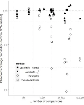
Figure 1
466
The observed coverage probability for nominal 95% confidence intervals plotted against the 467
number of comparisons, J, used in the calculation. No rare alleles are discarded (pcrit=0). The new
468
methods (filled shapes) while often over-conservative, hold up better than the existing ones 469
(hollow shapes) when J is extremely high. Note the logged scaled on the x-axis 470
471 472 473
Figure 2
474
The observed coverage probability for nominal 95% confidence intervals plotted against the 475
number of comparisons, J, used in the calculation. Alleles with observed frequencies less than 0.05 476
have been removed (Pcrit = 0.05). The performance of the new methods do not drop off as J
477
increases as much as the Pcrit = 0 case. This figure corresponds to the data shown in Table 2.
478
479
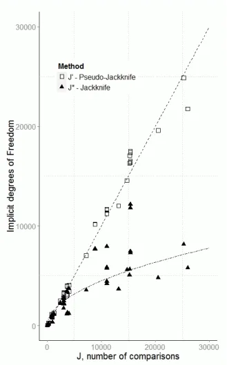
Figure 3
480
The number of degrees of freedom calculated for each of the two jackknife methods against the 481
nominal J value taken from the actual number of comparisons. The Pseudo-jackknife values appear 482
approximately proportional to the number of comparisons J. 483
The true jackknife values appear to be proportional to the square root of J, a simple linear 484
regression fitted to square root of the implicit degrees of freedom for the true jackknife is shown for 485
illustration(dotted line). 486
In the case of the parametric method the number of degrees of freedom is simply J, so the 487
value lies exactly on the top dashed line. 488
489