Pixel-Based Teeth Classification Using Dental
Panoramic X - Ray Images with Machine Learning
Methods
Ali GUVEN
Department of Electrical and Electronic Engineering, MS Student Economy and Technology University of TOBB
Sogutozu, Cankaya / Ankara, TURKEY Email: [email protected]
Abstract—Today many people suffer from dental diseases. Identifying the diseases is hard and takes time for doctors. Teeth classification from the X-Ray image becomes important to determine these diseases. Elimination of the pixels, that are not contains teeth pixels, from the image makes easy to understand disorders. So pixel-based elimination is used for this problem. By Using machine learning methods that are Extreme Gradient Boosting (XGB), Light Extreme Gradient Boosting (LXGB),and Cat Boosting training data set is learned. To measure the performance of the methods, accuracy scores are compared.
Index Terms—Dental Classification, Teeth Classification, Panoramic X-Ray, Machine Learning, Deep Learning
I. INTRODUCTION
The images have irrelevant pixels that do not belong to teeth. For example, bones, lips or flesh. Also pixel intensity values are same to each other. So that images have got high bias and much outliers. Elimination of bias and outliers is a np-hard problem. Classification of this irrelevant pixels and showing the teeth without them help doctors to determine the disorders. In the future, it may be a base tool for segmentation teeth and showing the disorders in seconds without supervisor. The main goal is classifying teeth with high accuracy like above 90 percent. Using the newest algorithms for machine learning is new according to the other related articles.
II. RELATEDWORKS
The general approach to pixel-based image classification problems is to apply image processing methods and then use K-means or Support Vector Machines (SVM) or KNN classi-fiers to determine if the pixel belongs to teeth or not. Used image processing methods are Scale-Invariant Feature Trans-form (SIFT), and Histogram of Oriented Gradients (HOG). Both make a bag-of-words pipeline for the machine learning methods, SVM and KNN. The words act like features or predictors and each pixels act like sample. The dataset is prepared by doing these processes. The another approach to classify the pixels is Convolutional Neural Network. Using CNN, it is much easier than other to eliminate the irrelevant pixels than others. However, CNN has black box and there is no explanation for added neuron number or used layer
on optimization the hyper parameters of SVM or KNN and on selection of features. In the references [1], it is given the recent published article of this problem. The classes of this problems 1 (teeth) and 0 (not teeth).
III. PREPARATION OFDATASET
The dataset is not open to public. It is given for research to solve this problem by using machine learning methods. So that, it is limited by 50 images. The dataset is prepared by this images. First some of them is tagged manually as drawing the teeth and assign 1 to tooth’s pixels and the other pixels are 0. The target (class) vector is prepared like that. The main problem of preparing dataset like the other problems is selection and determination of features.
A. Feature Determination
Determination of features is doing by image processing. Many identical features can be found. The most common of them are intensity, intensity of texture of image, and location of region of interest fields. The texture of image has many ways. One of them is using kernel and convolve the image with it then use the subtraction of maximum value and minimum value. The another is looking the variance of the same process.
B. Feature Selection
Selection of features is doing by principal component anal-ysis (PCA). For this problem, at the beginning, there are five features that are intensity of each pixels, texture of image by looking subtraction between maximum intensity value and minimum intensity value of convolution of kernel and image, texture of image by looking variance values of convolution of kernel and image, and location of region of interest. PCA uses the variance of features and eliminates the feature or features that has the least variance. By doing PCA, the texture of image by looking variance values of convolution of kernel and image has the least variance value and is eliminated from the dataset. The largest variance is faced in location of region of interest, intensity of image and texture of image by looking subtraction between maximum intensity value and minimum
GSJ: Volume 7, Issue 11, November 2019, Online: ISSN 2320-9186
1) Intensity Value of Image: It is looking the intensity value of each pixel and using as a feature. Using this feature is meaningless to classify teeth, because image has high bias. There are many irrelevant pixels that have same intensity value of tooth’s.
2) Texture of Image by Looking Subtraction between Maxi-mum Intensity Value and MiniMaxi-mum Intensity Value of Convolu-tion of Kernel and Image: It is looking the subtraction between the maximum intensity value and the minimum intensity value in the window by using kernel (filter) or without using kernel. This acts like high-pass filter for image.
3) Location of Region of Interest: This feature is separated into two independent feature. One of them is the x-axis coordinate of region of interest and the other one is y-axis coordinate of region of interest. That is the most important feature at all. User manually draws region of interest that includes all teeth. After the drawing, the center point of the region is automatically found and coordinate system has appeared.
IV. METHODS
1) Extreme Gradient Boosting (XGB)
XGBoost is an ensemble learning method. Ensemble learning offers a systematic solution to combine the predictive power of multiple learners. The resultant is a single model which gives the aggregated output from several models. The models that form the ensemble, also known as base learners, could be either from the same learning algorithm or different learning algorithms. Bagging and boosting are two widely used ensemble learners. Though these two techniques can be used with several statistical models, the most predominant usage has been with decision trees. Decision trees are said to be associated with high variance due to this behavior. Bagging or boosting aggregation helps to reduce the variance in any learner. Several decision trees which are generated in parallel, form the base learners of bagging technique. Data sampled with replacement is fed to these learners for training. The final prediction is the averaged output from all the learners. In boosting, the trees are built sequentially such that each subsequent tree aims to reduce the errors of the previous tree. Each tree learns from its predecessors and updates the residual errors. Hence, the tree that grows next in the sequence will learn from an updated version of the residuals. Having a large number of trees might lead to overfitting. So, it is necessary to carefully choose the stopping criteria for boosting. XGBoost is a popular implementation of gradient boosting. Unique features of XGBoost are regularization, handling sparse data, weighted quantile sketch, block structure for parallel learning, cache awareness, and out-of-core computing. XGBoost has an option to penalize complex models through both L1 and L2. Missing values or data pro-cessing steps like one-hot encoding make data sparse.
XGBoost incorporates a sparsity-aware split finding al-gorithm to handle different types of sparsity patterns in the data. Most existing tree based algorithms can find the split points when the data points are of equal weights (using quantile sketch algorithm). However, they are not equipped to handle weighted data. XGBoost has a distributed weighted quantile sketch algorithm to effectively handle weighted data. For faster computing, XGBoost can make use of multiple cores on the CPU. This is possible because of a block structure in its system design. Data is sorted and stored in in-memory units called blocks. Unlike other algorithms, this enables the data layout to be reused by subsequent iterations, instead of computing it again. This feature also serves useful for steps like split finding and column sub-sampling. In XGBoost, non-continuous memory access is required to get the gradient statistics by row index. Hence, XGBoost has been designed to make optimal use of hardware. This is done by allocating internal buffers in each thread, where the gradient statistics can be stored. This feature optimizes the available disk space and maximizes its usage when handling huge datasets that do not fit into memory.
2) Light Extreme Gradient Boosting (LXGB)
LightGBM uses histogram-based algorithms, which bucket continuous feature (attribute) values into discrete bins. This speeds up training and reduces memory us-age. Advantages of histogram-based algorithms include reduced cost of calculating the gain for each split, use histogram subtraction for further speedup, reduce memory usage, reduce communication cost for parallel learning. LightGBM grows trees leaf-wise (best-first). It will choose the leaf with max delta loss to grow. Holding number leaf fixed, leaf-wise algorithms tend to achieve lower loss than level-wise algorithms. Leaf-wise may cause over-fitting when data is small, so LightGBM includes the max depth parameter to limit tree depth. However, trees still grow leaf-wise even when max depth is specified.
3) Cat Boost
provides state of the art results and it is competitive with any leading machine learning algorithm on the performance front. CatBoost converts categorical values into numbers using various statistics on combinations of categorical features and combinations of categorical and numerical features. It reduces the need for ex-tensive hyper-parameter tuning and lower the chances of overfitting also which leads to more generalized models. Although, CatBoost has multiple parameters to tune and it contains parameters like the number of trees, learning rate, regularization, tree depth, fold size, bagging temperature and others.
V. RESULTS ANDDISCUSSION
The training dataset is prepared for seven image of dental panoramic X-Ray. The model is created by this training dataset and tested by two example image. The results are listed below for each method.
A. XGB Results
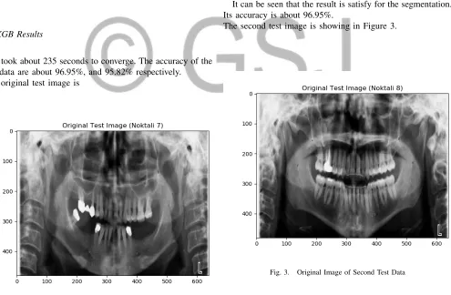
It took about 235 seconds to converge. The accuracy of the test data are about 96.95%, and 95.82% respectively.
The original test image is
Fig. 1. Original Image of First Test Data
The XGB result for the test data is showing in Figure 2.
Fig. 2. XGB Result for the Image of First Test Data
It can be seen that the result is satisfy for the segmentation. Its accuracy is about 96.95%.
The second test image is showing in Figure 3.
Fig. 3. Original Image of Second Test Data
Fig. 4. XGB Result for the Image of Second Test Data
It can be seen that the result is satisfy for the segmentation. Its accuracy is about 96.95%.
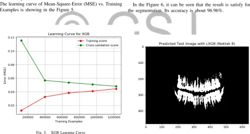
The learning curve of Mean-Square-Error (MSE) vs. Training Examples is showing in the Figure 5.
Fig. 5. XGB Learning Curve
B. LXGB Results
It took about 38 seconds to converge. The accuracy of the test data are about 96.96%, and 95.78% respectively.
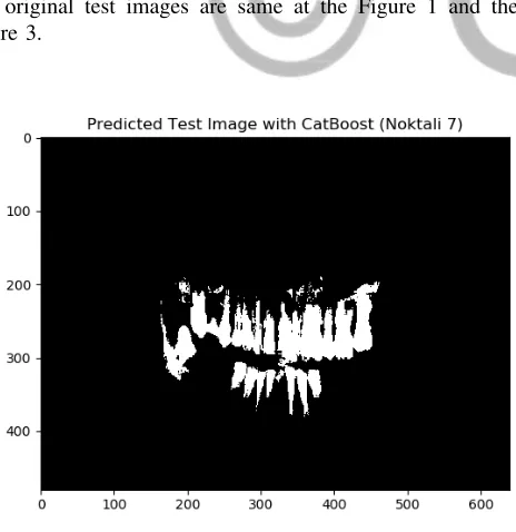
The original test images are same at the Figure 1 and the Figure 3.
Fig. 6. LXGB Result for the Image of First Test Data
In the Figure 6, it can be seen that the result is satisfy for the segmentation. Its accuracy is about 96.96%.
Fig. 7. LXGB Result for the Image of Second Test Data
Fig. 8. LXGB Learning Curve
The results of LGBX is almost same as the results of XGB. LXGB takes less time than XGB does.
C. Cat Boost Results
It took about 39 seconds to converge because of using GPU. The accuracy of the test data are about 97.17%, and 95.94% respectively.
The original test images are same at the Figure 1 and the Figure 3.
Fig. 9. Cat Boost Result for the Image of First Test Data
In the Figure 9, it can be seen that the result is satisfy for the segmentation. Its accuracy is about 97.17%.
Fig. 10. Cat Boost Result for the Image of Second Test Data
In the Figure 10, it can be seen that the result is satisfy for the segmentation. Its accuracy is about 95.94%.
Fig. 11. Cat Boost Learning Curve
Cat Boost is much better than the other methods. According to both elapsed time and accuracy score, Cat Boost performs well.
VI. CONCLUSIONS
TABLE I
TABLE OFTHEACCURACYSCORES OFTHEMODELS
Number of Test Image XGB LXGB Cat Boost
1 96.95% 96.96% 97.17%
2 95.82% 95.78% 95.94%
REFERENCES
[1] Yu, Young-junMachine Learning for Dental Image Analysis.2016: eprint arXiv:1611.09958.
[2] An End-to-End Guide to Understand the Math behind XGBoost.
URL: https://www.analyticsvidhya.com/blog/2018/09/an-end-to-end-guide-to-understand-the-math-behind-xgboost/ (accessed: September 6, 2018).
[3] Welcome to LightGBM’s documentation!. URL: https://lightgbm.readthedocs.io/en/latest/Features.html (accessed: 2019). [4] Ray, Sunil.CatBoost: A machine learning library to