A
Variable
N
eighborhood
S
earch
A
lgorithm
for
S
olving
the
S
teiner
M
inimal
T
ree
P
roblem
in
S
parse
G
raphs
C.V. Tran
1,*, N. H. Ha
21The Center for Information Technology and Communication, 284 Tran Hung Dao Street, Ca Mau City, Vietnam
2Research Institute of Posts and Telecommunications (RIPT), 122 Hoang Quoc Viet Street, Ha Noi City, Vietnam
Abstract
Steiner Minimal Tree (SMT) is a complex optimization problem that has many important applications in science and technology; This is a NP-hard problem. Much research has been carried out to solve the SMT problem using approximate algorithms. This paper presents A Variable Neighborhood Search (VNS) algorithm for solving the SMT problem in sparse graphs; The proposed algorithm has been tested on sparse graphs in a standardized experimental data system, and it yields better results than some other heuristic algorithms.
Keywords: Minimal tree, sparse graph, variable neighborhood search algorithm, metaheuristic algorithm, Steiner minimal tree.
Received on 01 December 2018, accepted on 07 December 2018, published on 10 December 2018
Copyright © 2018 C.V. Tran and N. H. Ha, licensed to EAI. This is an open access article distributed under the terms of the Creative Commons Attribution licence (http://creativecommons.org/licenses/by/3.0/), which permits unlimited use, distribution and reproduction in any medium so long as the original work is properly cited.
doi: 10.4108/eai.6-2-2019.156534
A preliminary version of this work under the title “A Variable Neighborhood Search Algorithm for Solving the Steiner Minimal Tree Problem” has appeared in the proceedings of the 7th EAI International Conference, ICCASA 2018 and 4th EAI International Conference, ICTCC 2018 in Viet Tri City, Vietnam, November 22–23, 2018.
1.
1.1. Definitions
This section presents several definitions and properties associated with the Steiner minimal tree problem.
Definition 1. Steiner tree [2]
Let’s assume that G = (V(G), E(G)) is a simple undirected connected graph with non-negative weight on the edge; V(G)
is the set of n vertices, E(G) is a set of m edges, w(e) is the weight of edge e, e ∈ E(G). Assume that L is a subset of vertices of V(G); Tree T passing through all vertices in L is called Steiner tree's L.
The set L is called the terminal set, the vertices in the set L
are called the terminal vertices; the vertices in the T trees that
are not in the set L are called the Steiner vertices. Unlike most common spanning tree problems, the Steiner tree just passes
Introduction
through all the vertices in the terminal set L and some othervertices in the set V(G).
Definition 2. Cost of Steiner tree [2]
Let T = (V(T), E(T)) is a Steiner tree of graph G, cost of the tree T, denoted by C(T), is the total weight of the edges of the tree T, i.e.𝐶(𝑇) = ∑𝑒∈𝐸(𝑇)𝑤(𝑒)
Definition 3. Steiner Minimal Tree [2]
Given the graph G, the problem of finding Steiner Trees with Minimal Cost is defined as the Steiner Minimal Tree problem – SMT or more concisely as Steiner Tree Problem.
In this paper, the word graph is used to describe a connected undirected graph with the non-negative weights.
1.2. Application of SMT problem
The SMT problem has important applications in different fields of science and technology. For example, it has been applied in network design, circuit layout…SMT problem is
NP-hard [6,7], and hence its applications are fallen into two different perspectives: design and execution. Design problems favor the quality of the solution while running time is more prioritized for execution problems [1,3,8,11].
1.3. Related work
The SMT problem has attracted the academic attention of many scientists in the world over the past decades; There have been different algorithms for solving SMT problem that can be divided into the following approaches:
The first approach is the algorithms for finding the correct solution. Algorithms of this class are dynamic programming, augmented Lagrangian-based algorithms, Branch and Bound Algorithm, etc.. One of the advantages of this approach is that correct solutions can be found. However, this class of algorithms is only suitable for the small-sized problems. The algorithms with correct solutions can be used for benchmarking the accuracy of approximation algorithms. Finding a correct solution to the SMT problem is a big challenge in combinatorial optimization theory [4,6].
The second approach is the class of heuristic algorithms. Heuristic algorithms make use of individual experiences for finding solutions to a particular optimization problem. Heuristic algorithms yield acceptable solutions, which might not be the best solution, in the permissible time. Optimal running time can be achieved with this class of algorithms [9,10,11].
The third approach is metaheuristic algorithms. The metaheuristic algorithms use a variety of heuristic algorithms in combination with auxiliary techniques to exploit the search space; The metaheuristic algorithm belongs to the class of optimal search algorithms. There have been already a number of different projects employed the metaheuristic algorithms for solving the SMT problem such as local search algorithms, Tabu search algorithms, genetic algorithms, parallel genetic algorithms, etc. Up to the present, the metaheuristic approach provides high quality solutions among approximation algorithms [13,14]; However, the execution time of the metaheuristic algorithms is much slower than that of the heuristic algorithms.
This paper presents a metaheuristic approximation algorithm that is a VNS algorithm for solving the SMT
problem in sparse graphs, a preliminary version of this work under the title “A Variable Neighborhood Search Algorithm for Solving the Steiner Minimal Tree Problem” [16].
2. VNS algorithm for solving SMT problem
2.1. Using the variable neighborhood search
Node-Base (Node-Based) [12]
Input: Let G=(V(G), E(G)) be an undirected graph with V - a set of vertices, E - a set of edges; L ⊆V - a set of terminal vertices.
Output: A minimum Steiner tree T
Use Like Prim’s algorithm to search a spanning tree in the graph, T is a tree;
Remove redundant edges of T, then T is a Steiner tree, proceed as follows: With each Steiner tree T, browse all pendant vertices u∈T, if u∉L, delete edge containing vertex
ufrom E(T), delete vertex u in V(T) and update the vertex’s
degree which is adjacent to vertex u in T. Repeat this procedure until T is unchanged.
while (stop condition is not satisfied) {
Let T1=T;
Select random vertex u ∈ T1; the vertex u which doesn’t belong to a set of terminal vertices L; then, remove the edges related to the vertex u in T1; when T1 is divided into more connected parts; that graph is T2.
Arrange the edges of the G – graph by ascendant weights, add the edges in the order sorted in G to the graph T2until T2 is a tree;
Remove redundant edges in T2;
If the tree T2 is lighter weight than T, replace T by T2; vice versa, if the tree T2 is not created, let T be T1;
}
2.2. Using the variable neighborhood search
Path Based (Path-Based) [13]
A key-node is a Steiner node with degree of 3 at the lowest. A key-path is one with all intermediate vertices (not be terminal vertex) with degree 2, the first and the last vertex of that path or belong to a set of terminal vertices or become a key-node. Searching a random key-path proceeds as follows: Select a random edge in T; if the first and the last vertex are ones with degree 2 and they and Steiner vertices, add the next adjacent edge of that vertex until the first and the last vertex have degree not equal to 2 and they are not Steiner vertices, check if the path is a key-path or not. Stop if stop condition is met. Using Like Prim’s algorithm to search the Steiner of tree, T
is a tree;
Remove redundant edges of T, then T is a Steiner tree; while (stop condition is not satisfied)
{ Let T1=T;
Suppose that p is a random key-path; proceed removing
p; then T is divided into two components Ta and Tb;
Select the minimum-weight edge which connects two components Ta and Tb; suppose we have a new tree T2.
If the tree T2 is lighter weight than T, replace T by T2; vice versa, if T2 doesn’t exist, let T be T1;
}
Stop condition: Stop condition is considered to be met if the best solution cannot be improved by after a predefined number of iterations t.
Initial condition: Each spanning tree is created by using Prim's algorithm described as: initialize a tree with a single vertex chosen arbitrarily from the graph. the algorithm will be iterated for n-1 times. In each iteration, grow the tree by adding a vertex that is adjacent to at least one vertex of the spanning tree without consideration of its weight and its connected edges to the spanning tree. This algorithm is named as Like Prim’s algorithm.
Like Prim (V, E)
Input: Graph G = (V(G), E(G))
Output: Return a random spanning tree T = (V(T), E(T))
1. Choose a vertex u ∈ V(G); 2.V(T) = {u};
3.E(T) = ∅;
4. while (|V(T)| < n) {
5. Choose a vertex v ∈ V(G) – V(T)v is an adjacent vertex of a vertex z ∈ V(T);
6. V(T)= V(T) ∪ {v};
7. E(T)= E(T) ∪ {(v, z)};
8.}
9. return spanning tree T;
Run the Like Prim's algorithm separately for each connected component and/or connected components of the graph or to find the minimum spanning forest in heuristic and metaheuristic algorithm to solve SMT problem. The advantage of Like Prim's algorithm in comparison with heuristic algorithms in providing an initial solution is the variety of edges of the spanning tree. The quality of the initial population created by Like Prim's algorithm is not so good as that of the initial population created by heuristic algorithms. However, after the evolutionary process, spanning trees created by Like Prim's algorithm usually provide better quality solutions.
Step – form of VNS algorithm to solve SMT problem:
T is a spanning tree which is formed by Like Prim algorithm.
Remove redundant edges.
Get the Steiner tree by removing redundant edges in T; While (The stop condition is not true)
{
- Execute 2 variable neighborhood search Node-based and Path-based one by one;
- Record the better solution;
- While executing VNS algorithm, if a better solution is found, execute VNS algorithm from the beginning (after while loop) and vice versa, continue to the next VNS algorithm;
- VNS algorithm stops when stop condition is met. The stop condition in this particularly algorithm is the number of iterations, which is 10*n in this case, n is the number of vertices in the graph.
}
Return to the best solution.
3. Experiments
3.1. Experimental data
Experiment has been conducted to evaluate related algorithms. 78 sets of data have been selected from the standard experimental database for benchmarking algorithms for solving the Steiner tree problem. The data set can be found at URL:
http://people.brunel.ac.uk/~mastjjb/jeb/orlib/steininfo.html [5]. 18 graphs are from group steinb, 20 graphs are from group steinc, 20 graphs are from group steind and the other 20 graphs come from steine.
3.2. Experimental environment
The MST-Steiner, SPT-Steiner, PD-Steiner, Node-based, Path-based algorithm and VNS algorithm are implemented in C++, DEV C++ 5.9.2; experimented on a Virtual Server Windows server 2008 R2 Enterprise, 64bit, Intel(R) Xeon (R) CPU E5-2660 @ 2.20 GHz, RAM 4GB.
3.3. Experimental results and evaluation
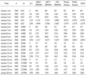
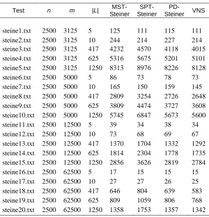
Experimental results of algorithms are given in Tables 1, 2, 3, 4. The tables are structured as follows: The first column (Test) is the name of the data sets in the experimental data system; number of vertices (n), number of edges (m) and number of vertices in the terminal vertices (|L|) of each graph; The next column records the Steiner tree’s cost value corresponding to the MST-Steiner, SPT-Steiner, PD-Steiner or Node-based, Path-based and Variable Neighborhood Search algorithm (VNS).
Table 1. Experimental algorithm results on the steinb
graph group
Test n m |L| MST-Steiner
SPT-Steiner
PD-Steiner VNS
steinb13.txt 100 125 17 175 172 175 165 steinb14.txt 100 125 25 237 253 235 236 steinb15.txt 100 125 50 323 335 318 318 steinb16.txt 100 200 17 137 138 133 127 steinb17.txt 100 200 25 134 139 132 131 steinb18.txt 100 200 50 222 250 222 218
Table 2. Experimental algorithm results on the steinc graph group
Test n m |L| MST-Steiner
SPT-Steiner
PD-Steiner
Node-based
Path-based VNS
steinc1.txt 500 625 5 88 86 85 85 85 85
steinc2.txt 500 625 10 144 158 144 144 144 144 steinc3.txt 500 625 83 779 843 762 754 754 754 steinc4.txt 500 625 125 1114 1193 1085 1079 1079 1079 steinc5.txt 500 625 250 1599 1706 1583 1579 1579 1579 steinc6.txt 500 1000 5 60 56 55 55 55 55 steinc7.txt 500 1000 10 115 103 102 102 103 102 steinc8.txt 500 1000 83 531 597 516 509 509 509 steinc9.txt 500 1000 125 728 865 718 707 707 707 steinc10.txt 500 1000 250 1117 1327 1107 1093 1093 1093 steinc11.txt 500 2500 5 37 32 34 32 33 33 steinc12.txt 500 2500 10 49 46 48 46 46 46 steinc13.txt 500 2500 83 274 322 268 258 258 258 steinc14.txt 500 2500 125 337 417 332 323 323 323 steinc15.txt 500 2500 250 571 703 562 556 556 556 steinc16.txt 500 12500 5 13 12 12 11 11 11 steinc17.txt 500 12500 10 19 19 20 18 18 18 steinc18.txt 500 12500 83 125 146 123 116 116 115 steinc19.txt 500 12500 125 158 195 159 147 147 148 steinc20.txt 500 12500 250 269 339 268 267 268 268
Table 3. Experimental algorithm results on the steind graph group
Test n m |L| MST-Steiner
SPT-Steiner
PD-Steiner
Node-based
Path-based VNS
steind12.txt 1000 5000 10 43 44 42 42 42 42 steind13.txt 1000 5000 167 531 643 518 501 502 502 steind14.txt 1000 5000 250 702 851 691 669 667 671 steind15.txt 1000 5000 500 1151 1437 1134 1117 1120 1116 steind16.txt 1000 25000 5 15 13 14 13 13 13 steind17.txt 1000 25000 10 25 25 23 23 23 23 steind18.txt 1000 25000 167 251 301 246 228 228 228 steind19.txt 1000 25000 250 344 424 334 313 317 318 steind20.txt 1000 25000 500 544 691 542 537 539 538
Table 4. Experimental algorithm results on the steine graph group
Test n m |L| MST-Steiner
SPT-Steiner
PD-Steiner VNS
steine1.txt 2500 3125 5 125 111 115 111 steine2.txt 2500 3125 10 244 214 227 214 steine3.txt 2500 3125 417 4232 4570 4118 4015 steine4.txt 2500 3125 625 5316 5675 5201 5101 steine5.txt 2500 3125 1250 8313 8976 8226 8128 steine6.txt 2500 5000 5 86 73 78 73 steine7.txt 2500 5000 10 165 150 159 145 steine8.txt 2500 5000 417 2809 3254 2726 2648 steine9.txt 2500 5000 625 3809 4474 3727 3608 steine10.txt 2500 5000 1250 5745 6847 5673 5600 steine11.txt 2500 12500 5 39 34 38 34 steine12.txt 2500 12500 10 73 68 69 67 steine13.txt 2500 12500 417 1370 1704 1332 1292 steine14.txt 2500 12500 625 1814 2304 1778 1735 steine15.txt 2500 12500 1250 2856 3626 2819 2784 steine16.txt 2500 62500 5 17 15 15 15 steine17.txt 2500 62500 10 27 27 26 25 steine18.txt 2500 62500 417 646 804 639 583 steine19.txt 2500 62500 625 809 1059 806 768 steine20.txt 2500 62500 1250 1358 1753 1357 1342
This section aims to compare the solution quality of VNS algorithm with the group of MST-Steiner, SPT-Steiner, PD-Steiner algorithm [15] and group of Node-based, Path-based algorithm [12].
With 20 sets of data in steinb group, the VNS algorithm offers a better solution quality at 72.2%, equivalent quality at 22.2% and worse quality at 5.6% in comparison with MST-Steiner algorithm. The VNS algorithm offers a better solution quality at 77.8%, equivalent quality at 16.7% and worse quality at 5.6% in comparison with SPT-Steiner algorithm. The VNS algorithm offers a better solution quality at 50.0%, equivalent quality at 44.4% and worse quality at 5.6% in comparison to PD-Steiner algorithm.
With 20 sets of data in steinc group, the VNS algorithm offers a better solution quality at 5%, equivalent quality at
based algorithm. The VNS algorithm offers a better solution quality at 10%, equivalent quality at 85% and worse quality at 5% in comparison with Path-based algorithm. The VNS algorithm offers a better solution quality at 95%, equivalent quality at 5% and worse quality at 0% in comparison with MST-Steiner algorithm. The VNS algorithm offers a better solution quality at 90%, equivalent quality at 5% and worse quality at 5% in comparison with SPT-Steiner algorithm. The VNS algorithm offers a better solution quality at 75%, equivalent quality at 25% and worse quality at 0% in comparison to PD-Steiner algorithm.
Node-solution quality at 30%, equivalent quality at 60% and worse quality at 10% in comparison with Path-based algorithm. The VNS algorithm offers a better solution quality at 100%, equivalent quality at 0% and worse quality at 0% in comparison with MST-Steiner algorithm. The VNS algorithm offers a better solution quality at 90%, equivalent quality at 10% and worse quality at 0% in comparison with SPT-Steiner algorithm. The VNS algorithm offers a better solution quality at 85%, equivalent quality at 15% and worse quality at 0% in comparison to PD-Steiner algorithm.
With 20 sets of data in steine group, the VNS algorithm offers a better solution quality at 100%, equivalent quality at 0% and worse quality at 0% in comparison with MST-Steiner algorithm. The VNS algorithm offers a better solution quality at 75%, equivalent quality at 25% and worse quality at 0% in comparison with SPT-Steiner algorithm. The VNS algorithm offers a better solution quality at 95%, equivalent quality at 5% and worse quality at 0% in comparison to PD-Steiner algorithm.
4. Conclusions
In this paper, the VNS algorithm has been proposed to solve SMT problem in sparse graphs; The proposed algorithm has been experimentally implemented and evaluated using 78 sets of data as sparse graphs in the standard experimental datasets. The experiment outcomes show promising results in which the solution quality provided by the proposed algorithm is significantly improved compared to MST-Steiner, SPT-Steiner, PD-Steiner, Node-based and Path-based algorithm.
References
[1] Koster, A., Munoz, X. (2010) Graphs and Algorithms in Communication Networks. Springer.
[2] Wu, B, Y., Chao, K. (2004) Spanning Trees and Optimization Problems. Chapman&Hall/CRC: pp.158–165. [3] Lu, C, L., Tang, C, Y. (2003) The full Steiner tree problem.
ELSEVIER: pp.55-67.
[4] Una, D, D., Gange, G., Schachte, p., Stuckey, P, J. (2016) Steiner Tree Problems with Side Constraints Using Constraint Programming. Proceedings of the Thirtieth AAAI Conference on Artificial Intelligence.
[5] Beasley J. E., OR-Library: URL, http://people.brunel.ac.uk/~mastjjb/jeb/orlib/steininfo.html, last accessed 2018.
[6] Laarhoven, J, W, V. (2010) Exact and heuristic algorithms for the Euclidean Steiner tree problem. University of Iowa, Doctoral thesis.
[7] Caleffi, M., Akyildiz, I, F., Paura, L. (2015) On the Solution of the Steiner Tree NP-Hard Problem via Physarum BioNetwork. IEEE: pp.1092-1106.
[8] Hauptmann, M., Karpinski, M. (2015) A Compendium on Steiner Tree Problems: pp.1-36.
[9] Hougardy, S., Silvanus, J., Vygen, J. (2015) Dijkstra meets Steiner: a fast exact goal-oriented Steiner tree algorithm. University of Bonn.
[10] Bosman, T. (2015) A Solution Merging Heuristic for the Steiner Problem in Graphs Using Tree Decompositions. VU University Amsterdam, Netherlands: pp.1-12.
[11] Cheng, X., Du, D, Z. (2004) Steiner trees in industry. Kluwer Academic Publishers, 5: pp.193-216.
[12] Martins, S, L., Resende, M.G.C., Ribeiro, C.C, Pardalos, P.M. (1999) A parallel grasp for the steiner tree problem in graphs using a hybrid local search strategy.
[13] Uchoa, E., Werneck, R, F. (2010) Fast Local Search for Steiner Trees in Graphs.
[14] Ribeiro, C, C., Mauricio, C., Souza, D. (2000) Tabu Search for the Steiner Problem in Graphs. Networks, 36: pp.138-146.
[15] C. V. Tran, Q. T. Phan, N. H. Ha. (2017) Heuristic Algorithms for solving Steiner Minimal Tree Problem. Proceedings of the 10th National Coference on Fundamental
and Applied Information Technology Research (FAIR’10): pp. 138-147.