R E S E A R C H A R T I C L E
Open Access
Optimum binary cut-off threshold of a diagnostic
test: comparison of different methods using
Monte Carlo technique
Gilbert Reibnegger
*and Walter Schrabmair
Abstract
Background:Using Monte Carlo simulations, we compare different methods (maximizing Youden index, maximizing mutual information, and logistic regression) for their ability to determine optimum binary cut-off thresholds for a ratio-scaled diagnostic test variable. Special attention is given to the stability and precision of the results in dependence on the distributional characteristics as well as the pre-test probabilities of the diagnostic categories in the test population.
Methods:Fictitious data sets of a ratio-scaled diagnostic test with different distributional characteristics are generated for 50, 100 and 200 fictitious“individuals”with systematic variation of pre-test probabilities of two diagnostic categories. For each data set, optimum binary cut-off limits are determined employing different methods. Based on these optimum cut-off thresholds, sensitivities and specificities are calculated for the respective data sets. Mean values and SD of these variables are computed for 1000 repetitions each.
Results:Optimizations of cut-off limits using Youden index and logistic regression-derived likelihood ratio functions with correct adaption for pre-test probabilities both yield reasonably stable results, being nearly independent from pre-test probabilities actually used. Maximizing mutual information yields cut-off levels decreasing with increasing pre-test probability of disease. The most precise results (in terms of the smallest SD) are usually seen for the likelihood ratio method. With this parametric method, however, cut-off values show a significant positive bias and, hence, specificities are usually slightly higher, and sensitivities are consequently slightly lower than with the two non-parametric methods.
Conclusions:In terms of stability and bias, Youden index is best suited for determining optimal cut-off limits of a diagnostic variable. The results of Youden method and likelihood ratio method are surprisingly insensitive against distributional differences as well as pre-test probabilities of the two diagnostic categories. As an additional bonus of the parametric procedure, transfer of the likelihood ratio functions, obtained from logistic regression analysis, to other diagnostic scenarios with different pre-test probabilities is straightforward.
Background
Evaluation of diagnostic tests is an important issue in medical disciplines. Best known is the analysis of simple diagnostic test situations which can be represented by means of a 2 × 2-contingency table: one dimension of such a table is defined by two diagnostic categories (e.g., “non-diseased”versus“diseased”), and the second dimen-sion represents the dichotomous test result (e.g.,“normal” versus“pathological”). According to its importance, there
is a large literature on the subject. A recent series of review articles presents an excellent overview cover-ing all relevant theoretical and practical aspects of the subject [1-4].
An interesting way of evaluating diagnostic tests is provided by information theory [5-9], and an alternative elegant way of dealing with multiple, variably scaled diag-nostic variables, has been suggested in 1982 by Albert [10]: he demonstrated that logistic regression analysis can be employed to compute likelihood ratio functions which, in analogy to the well-known likelihood ratio ob-tained from a simple 2 × 2-contingency table, are useful to * Correspondence:[email protected]
Institute of Physiological Chemistry, Center of Physiological Medicine, Medical University of Graz, A-8010 Graz, Austria
compute post-test probability functions of the diagnostic categories investigated. A critical step when applying lo-gistic regression results for the computation of likelihood ratio functions is a correction according to the pre-test probabilities of the diagnostic categories actually used for the regression procedure [10]. A combination of Albert’s findings with a generalization of the computation of post-test probabilities for more than two diagnostic categories [11,12] was demonstrated [13].
In an attempt to (1) direct new awareness to Albert’s time-honoured but nevertheless most relevant results re-garding the use of logistic regression analysis in clinical chemistry, and to (2) compare logistic regression analysis with other methods for dividing patients into those with low versus those with high risk of being“diseased”, we here present the results of Monte-Carlo simulation studies. Spe-cifically, for a diagnostic dilemma (“diseased”versus“ non-diseased”) we simulate data sets for a fictitious diagnostic variable x with different pre-specified distributional charac-teristics for the two diagnostic categories. Then, we search for the optimum cut-off threshold of x including the fol-lowing methods:
maximizing the mutual information of the respective 2 × 2-contingency table obtained by systematically varying a binary cut-off threshold for the diagnostic variable x
maximizing the Youden index (Youden index = sensitivity + specificity−1) by systematically varying a binary cut-off threshold for the diagnostic variable x
performing a logistic regression analysis on the problem and searching the value of the diagnostic variable x for which the logistic regression-derived likelihood ratio (LR) function, properly corrected for the pre-test probabilities of the diagnostic categories used for the regression procedure, attains unity (i.e., the test value at which the post-test probabilities of the diagnostic categories equal the pre-test
probabilities).
Major results of the simulations investigated are, for each of these three statistical procedures, the respective optimum cut-off values as well as their associated sensi-tivities and specificities. Besides mean values of these quantities of central interest, important“by-products” of the Monte-Carlo approach are their SD observed over the repetitive computer experiments.
We perform such calculations for four scenarios using different distributional characteristics underlying the computer-generated test data. Besides employing dif-ferent sample sizes, as the most important additional con-trol variable pre-test probabilities of disease [P(D)] are systematically varied over a wide range (from 0.10 to 0.90).
With these Monte-Carlo simulation experiments we attempt to answer the following research questions:
How well are the two non-parametric methods (maximizing mutual information, maximizing Youden index) and the parametric method (LR technique based on logistic regression analysis) suited for determining optimum binary cut-off levels of a ratio-scaled diagnostic test, given different distributional characteristics of test data, and how well do the results of the three methods agree with the theoretical crossing points of the distribution functions underlying the two diagnostic categories?
How do total numbers of test data and their composition in terms of pre-test probabilities of the two diagnostic categories influence the results?
Which of the techniques yields the most precise estimates in terms of the resulting SD values of the Monte Carlo simulation runs?
Methods
All computations are done using the commercially avail-able computer software MATHEMATICA, version 9, by Wolfram Research, Inc., Champaign, IL, USA.
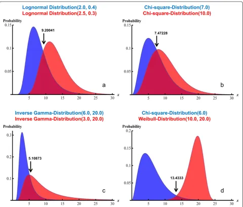
First, for the categories “no disease” and “disease”, according to P(D) chosen, fictitious patient data sets are generated using the random number generator of MATHEMATICA in combination with one out of many possible distribution functions: thus, for both diagnostic categories, fictitious data of a ratio-scaled diagnostic vari-able are generated following the chosen distribution func-tions. We choose total numbers of fictitious data sets of 50, 100 and 200, and we assume pre-test probabilities of category“disease”[P(D)] increasing from 0.10 to 0.90 in steps of 0.10. We simulate four different diagnostic scenarios:
Scenario 1: The lognormal distribution with mean value 2.0 and standard deviation 0.4 is assumed for the“healthy”category, and with mean value 2.5 and standard deviation 0.3 for the“diseased”category.
Scenario 2: The chi-square distribution with 7 degrees of freedom is assumed for the“healthy” category, and with 10 degrees of freedom for the “diseased”category.
Scenario 3: The inverse gamma distribution with shape parameter 6.0 is assumed for the“healthy” category and 3.0 for the“diseased”category. The scale parameter is set to 20.0 for both categories.
Using the MATHEMATICA function FindRoot, we obtain the following crossing points for the distribution functions of the two diagnostic categories: Scenario 1,
x= 9.20041; Scenario 2, x= 7.47228; Scenario 3; x= 5.10873; and Scenario 4, x= 13.4333. Differences from these values define the bias of the actually detected mean cut-off levels.
Analyses done on each data set include:
“Empirical”determination of the cut-off value at which mutual information is maximum (“Mutual information method”): the cut-off value is
systematically varied over the range of all test values by increments of 1.0, and that cut-off value is searched for which the resulting 2 × 2-contingency table produces the maximum mutual information.
Determination of the cut-off value at which Youden index is maximum. In the following, we shall designate this method as“Youden index method”. The cut-off value is systematically varied over the range of all test values by increments of 1.0, and that cut-off value is searched for which the resulting 2 × 2-contingency table produces the maximum Youden index.
Logistic regression analysis and calculation of the LR function (with proper correction for P(D) .
Determination of the test values for which the LR functions become equal to unity (“LR method”). Briefly, logistic regression analysis on a data set for N fictitious“individuals”yields a linear predictor functionα0 +α1 x, where x is the test result. The parametersα0 andα1 denote the intercept and the slope of the linear predictor. The linear predictor must be corrected for the pre-test probabilities of the diagnostic categories in order to yield the corrected linear predictor (equal to the natural logarithm of the LR function [10]):
logeð Þ ¼LR α0 þα1:x‐loge P Dð Þ 1‐P Dð Þ
;
the argument of the logarithm on the right side of the equation being the pre-test odds.
Thus, for each data set, according to each of these three methods, three cut-off limits as well as their asso-ciated sensitivities and specificities are computed as main results.
These analyses are repeated 1000 times in order to get not only estimates of these quantities of interest, but also“empirical”estimates for their SD values.
Additionally, the effects of P(D) on the parametersα0 andα1 as well as on the properly corrected intercept para-meter and, hence, on the post-test probabilities computed
thereof under different diagnostic situations, are demon-strated for a specific example.
For convenience, we supply the MATHEMATICA do-cuments necessary to reproduce our results: Additional file 1 (help.docx) gives a short explanation how to use the MATHEMATICA notebooks monte_carlo_SDev.nb (Additional file 2) which performs the necessary statis-tical calculations as well as the Monte Carlo simulation, and distributions.nb (Additional file 3) which produces graphical visualizations of the distribution functions used, and which calculates the crossing points of the two distri-bution functions for the“non-diseased”and the“diseased” fictitious individuals.
Results
The Monte Carlo experiments
For the Monte-Carlo experiments, we use the following conditions: total numbers of fictitious “individuals” are chosen as N =50, 100 and 200.
P(D) is varied, in steps of width 0.10, between P(D) =0.10 and P(D) =0.90.
At each P(D), 1000 data sets, each consisting of N =50, 100 or 200 randomly chosen test values x, are generated according to the four distributional scenarios detailed in the Methods section. Figure 1 demonstrates the distribu-tion funcdistribu-tions underlying the four scenarios.
Each data set contains N test values, of which N × P(D) values are associated with “Disease”, and N × [1−P(D)] values are labelled “No disease”. For each data set, the optimum cut-off threshold for x is determined by each of three different techniques (see Methods section).
Table 1 reports the ranges of the resulting mean values (and SD values) of the optimum cut-off values together with the associated sensitivities and specificities, obtained by the variation of P(D) from 0.1 to 0.9 in steps of 0.1.
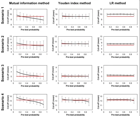
For the mean cut-off values and their SD values ob-tained with each of the three methods, Figure 2 demon-strates for the four scenarios the dependence on P(D) as well as the deviations with respect to the theoretical crossing points of the distribution functions underlying the two diagnostic categories. (Notably, each result is based on 200 fictitious individuals and 1000 repetitions.)
shows by far the smallest variations. On the other hand, the LR method tends to produce a constant positive bias; with the exception of Scenario 4 (strongly separated distri-bution functions underlying the two diagnostic categories) the cut-off levels found with this method lie consistently above the theoretical crossing points of the respective dis-tribution functions. In fact, the smallest bias is found with the Youden index method; with the Mutual information method cut-off levels at small P(D) are generally too high, and too low with high P(D).
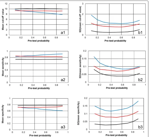
Figure 3 visualizes in more detail the results obtained for Scenario 1 (lognormal distributions with mean value 2.0 and standard deviation 0.4 for the“healthy”category, and with mean value 2.5 and standard deviation 0.3 for
the “diseased” category) and 200 fictitious “individuals” (N =200).
In accordance with Table 1 and Figure 2, the cut-off values and hence, the associated specificities, found by the LR method are usually slightly higher than those de-tected with the two non-parametric techniques. Con-sequently, the latter methods yield slightly better test sensitivities but slightly worse specificities than the LR method. As already shown in Figure 2 for the mean cut-off levels, also for sensitivities and specificities the stron-ger dependence of the Mutual information method on P(D) is clearly obvious from Figure 3 (panels a2 and a3). Analogously, also for the SD values of cut-off levels as well as of sensitivities and specificities the order LR
Chi-square-Distribution(7.0)
Chi-square-Distribution(10.0)
Lognormal Distribution(2.0, 0.4)
Lognormal Distribution(2.5, 0.3)
Inverse Gamma-Distribution(6.0, 20.0)
Inverse Gamma-Distribution(3.0, 20.0)
Chi-square-Distribution(6.0)
Weibull-Distribution(10.0, 20.0)
c
b
d
a
9.20041
7.47228
5.10873
13.4333
method < Youden index method < Mutual information method is obtained.
Closer inspection of the SD results in Table 1 shows in addition that in accordance with expectation, the variances of the results decrease with increasing sample size N.
Dependence on P(D) of the parametric estimates obtained by the LR-method
Despite the remarkable stability of the optimum cut-off thresholds as well as of sensitivities and specificities ob-tained by the parametric LR method over a broad range of P(D), the mean estimates of the logistic regression
Table 1 Results of the Monte Carlo simulations
N Mutual information Youden Likelihood ratio
Mean SD Mean Sd Mean SD
Scenario 1 (lognormal)
50
Cut-off 8.1 - 10.4 1.7 - 2.6 9.0 - 9.7 1.2 - 1.8 9.9 - 10.1 0.5 - 1.1
Se 0.78 - 0.86 0.17 - 0.30 0.82 - 0.91 0.10 - 0.14 0.74 - 0.76 0.08 - 0.16
Sp 0.69 - 0.76 0.18 - 0.23 0.73 - 0.82 0.12 - 0.17 0.78 - 0.78 0.06 - 0.14
100
Cut-off 8.1 - 10.0 1.4 - 2.2 9.2 - 9.5 1.0 - 1.4 10.0 - 10.10 0.4 - 0.7
Se 0.84 - 0.89 0.11 - 0.19 0.81 - 0.87 0.09 - 0.13 0.74 -0.75 0.05 - 0.11
Sp 0.65 - 0.74 0.15 - 0.22 0.72 - 0.78 0.09 - 0.15 0.78 - 0.78 0.04 - 0.10
200
Cut-off 7.8 - 9.7 1.1 - 1.9 9.2 - 9.4 0.8 - 1.1 10.0 - 10.1 0.3 - 0.5
Se 0.83 - 0.91 0.08 - 0.16 0.82 - 0.85 0.07 - 0.10 0.74 - 0.74 0.04 - 0.08
Sp 0.61 - 0.72 0.12 - 0.18 0.71 - 0.75 0.08 - 0.12 0.78 - 0.78 0.03 - 0.07
Scenario 2 (chi-square)
50
Cut-off 7.4 - 9.3 3.3 - 4.1 7.5 - 8.1 1.9 - 2.7 8.2 - 8.4 0.6 - 1.1
Se 0.67 - 0.70 0.26 - 0.35 0.69 - 0.80 0.17 - 90.21 0.59 - 0.61 0.08 - 0.17
Sp 0.62 - 0.73 0.24 - 0.30 0.65 - 0.77 0.17 - 0.22 0.69 - 0.70 0.07 - 0.15
100
Cut-off 7.4 - 9.0 3.1 - 4.1 7.5 - 8.0 1.5 - 2.2 8.3 - 8.4 0.4 - 0.8
Se 0.66 - 0.71 0.23 - 0.30 0.68 - 0.76 0.14 - 0.18 0.59 - 0.61 0.06 - 0.12
Sp 0.61 - 0.69 0.23 - 0.29 0.64 - 0.72 0.14 - 0.19 0.69 - 0.70 0.05 - 0.10
200
Cut-off 7.0 - 8.8 2.4 - 3.9 7.5 - 7.9 1.2 - 1.8 8.3 - 8.4 0.3 - 0.5
Se 0.67 - 0.72 0.20 - 0.27 0.67 - 0.72 0.12 - 0.16 0.59 - 0.60 0.04 - 0.09
Sp 0.59 - 0.65 0.21 - 0.26 0.63 - 0.67 0.12 - 0.17 0.69 - 0.70 0.03 - 0.07
Scenario 3 (inverse gamma)
50
Cut-off 5.1 - 7.1 1.7 - 2.6 5.1 - 5.8 0.9 - 1.6 5.4 - 5.8 0.5 - 0.9
Se 0.64 - 0.76 0.17 - 0.34 0.75 - 0.83 0.11 - 0.17 0.69 - 0.72 0.08 - 0.17
Sp 0.80 - 0.87 0.15 - 0.20 0.81 - 0.90 0.11 - 0.15 0.84 - 0.85 0.05 - 0.12
100
Cut-off 5.1 - 7.2 1.4 - 2.3 5.1 - 5.6 0.8 - 1.3 5.4 - 5.7 0.3 - 0.6
Se 0.63 - 0.76 0.15 - 0.27 0.75 - 0.79 0.09 - 0.14 0.69 - 0.71 0.06 - 0.12
Sp 0.81 - 0.87 0.12 - 0.19 0.81 - 0.85 0.09 - 0.13 0.84 - 0.85 0.04 - 0.08
200
Cut-off 5.1 - 7.2 1.1 - 2.2 5.1 - 5.3 0.6 - 1.0 5.5 - 5.6 0.2 - 0.5
Se 0.62 - 0.76 0.12 - 0.21 0.75 - 0.78 0.08 - 0.11 0.69 - 0.71 0.04 - 0.09
Sp 0.80 - 0.89 0.09 - 0.17 0.80 - 0.83 0.08 - 0.11 0.84 - 0.85 0.02 - 0.06
Scenario 4 (mixed)
50
Cut-off 9.9 - 14.2 1.6 - 2.5 10.4 - 14.1 1.6 - 2.9 12.1 - 14.6 1.1 - 1.8
Se 0.41 - 0.47 0.32 - 0.45 0.99 - 1.00 0.01 - 0.03 0.98 - 1.00 0.02 - 0.03
Sp 0.65 - 0.82 0.22 - 0.24 0.97 - 0.99 0.03 - 0.04 0.97 - 0.98 0.03 - 0.06
100
Cut-off 11.0 - 14.6 1.3 - 2.0 11.7 - 14.2 1.2 - 2.3 12.6 - 13.9 0.7 - 1.6
Se 0.48 - 0.69 0.43 - 0.47 0.98 - 1.00 0.02 - 0.02 0.98 - 0.99 0.02 - 0.03
Sp 0.79 - 0.94 0.13 - 0.23 0.97 - 0.98 0.02 - 0.04 0.97 - 0.97 0.02 - 0.05
200
Cut-off 11.4 - 14.6 1.0 - 1.4 12.5 - 13.9 0.9 - 1.7 13.1 - 13.6 0.5 - 1.2
Se 0.65 - 0.91 0.26 - 0.46 0.98 - 0.99 0.01 - 0.02 0.98 - 0.98 0.01 - 0.02
Sp 0.90 - 0.97 0.04 - 0.16 0.96 - 0.98 0.02 - 0.03 0.96 - 0.97 0.01 - 0.03
analyses (α0 and α1) nevertheless are somewhat depen-dent on P(D), and this dependence even remains after proper correction. For the example shown in Figure 3 [Scenario 1 (lognormal distributions with mean value 2.0 and standard deviation 0.4 for the “healthy” category, and with mean value 2.5 and standard deviation 0.3 for the “diseased” category) and 200 fictitious “individuals” (N =200)], at P(D) =0.10 the uncorrected mean intercept estimate (α0) is -5.246, and at P(D) =0.90 it increases to -3.075. Hence, the mean corrected intercept esti-mate decreases from -3.049 to -5.273 between these limits; and the mean slope estimates (α1) increases from 0.303 to 0.535. So in fact, also the corrected linear predictor functions (as well as the LR functions) change some-what according to P(D). How strongly influence these
dependencies the estimated post-test probabilities of dis-ease? To answer this question, the mean values of the Monte-Carlo estimates of the logistic regression analyses at P(D) =0.10, 0.50 and 0.90 were used to calculate three respective corrected LR functions. With each of these three functions, then, according to the fact that the post-odds can be computed by multiplication of the pre-post-odds
by the LR h1P D x‐ðP D xðjÞjÞ¼1P D‐ð ÞP Dð ÞLR xð Þi, we compute the
post-test probabilities P(D|x) (conditional probabilities for disease given test result x) as functions of test value x, again for three P(D) =0.10, 0.50 and 0.90.
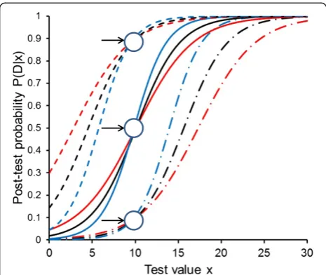
Figure 4 shows the resulting curves of the post-test probabilities. Notably, if the corrected estimates of the logistic regression analyses were independent from P(D)
Mutual information method Youden index method LR method
of the data set employed, the three LR functions would coincide, and we would finally obtain only three different and parallel sigmoid curves (one for each P(D) used for the second step of this computation). However, as the estimated slope parameters (α1) increase with increasing P(D) in the data sets used for the logistic regression ana-lyses, the sigmoidal post-test probability curves are steeper with respect to variation of test value x when we employ the estimates of logistic regression analyses obtained at higher P(D). Interestingly, each three curves obtained with
the three different sets of logistic regression estimates for a specified P(D) in the second calculation step (in Figure 4 these are the curves with the same line style each) cross at a test valuex≈10 and at a post-test probability which ap-proximates the actually specified P(D) (look at the little ar-rows in Figure 4).
Taking into account the results from Figure 2, we can easily understand this behaviour: Figure 3, panel a1, shows that with the LR method, a cut-off value ofx≈10 is obtained over the whole range of P(D). In other words,
a1
a2
a3
b1
b2
b3
at x ≈ 10, all three different LR functions yield approxi-mately unity, and hence, the post-test probabilities ap-proximate P(D).
In addition we note, that for each of the three different LR functions the respective set of three curves at differ-ent P(D) in the second calculation step (in Figure 4 these are the curves with the same colour) shows “parallel” course, due to their common slope parameter α1 being representative for the respective LR function.
Discussion
In this paper, we compare a parametric and two non-parametric methods of determining optimum binary cut-off levels of a ratio-scaled test using Monte Carlo technique. For scenarios with quite different distributio-nal characteristics underlying the computer-generated data sets, and for different total numbers of fictitious “individuals” (i.e., data sets), we focus on the effects of varying P(D) on the optimum cut-off levels obtained, and on sensitivities and specificities associated with these threshold values.
Our study shows that the Youden index method and the LR method yield very stable mean cut-off levels over the whole range of P(D), while the results of the Mutual information method show a characteristic monotonous decrease of the mean cut-off values with increasing P(D).
While the parametric LR method, based on logistic regres-sion analysis followed by proper correction of the inter-cept parameter for P(D), produces by far the most precise estimates (smallest SD values), the method yields results which are positively biased for three of the four distribu-tional scenarios studied. The best agreement between mean cut-off levels is obtained by the Youden index me-thod, and the worst precision (largest SD values) is gene-rally found by the technique of maximizing the mutual information statistic.
In perfect accordance with the behaviour of the mean optimum cut-off levels is the effect of the distributional scenarios as well as of P(D) on important test charac-teristics like sensitivities and specificities (and their SD values). Notably, as the LR technique generally produces the highest estimates of optimum cut-off levels (nearly irrespective of the distributional scenarios), it also yields the highest mean values for specificities, and in turn, the smallest mean values for sensitivities.
The estimates of the logistic regression analysis are somewhat dependent on the actual P(D) used, and post-test probability functions for the presence of disease, given a certain value of the diagnostic test variable, therefore show somewhat different slopes and positions; but as shown in Figure 4, the different curves obtained from lo-gistic regression analyses with different P(D), when ap-plied to compute post-test probabilities for a situation with an arbitrarily specified P(D) (in the second step), all cross approximately at a point in a P(D|x) vs. x diagram the abscissa of which is approximately equal to the op-timum cut-off value and the ordinate of which approxi-mates the specified P(D) (in the second step).
The results of the Monte Carlo simulations reported here appear to be representative for a broad variety of distributional characteristics underlying the test data in the“non-diseased”and the“diseased”category. Moreover, the results do not greatly vary when using 50, 100 or 200 fictitious“individuals”; clearly, the SD values obtained for increasing numbers of“individuals”are slightly decreasing. The study is restricted insofar as in any case, 1000 repeti-tions are employed for computing the respective mean values and SD values; however, this number is apparently high enough to guarantee quite stable estimates.
One might question the use of the crossing points of the involved distribution functions as the reference value for determining the bias of the methods: the crossing points of the distribution functions as used in our work imply a P(D) of 0.50 (both diagnostic categories would have the same weight) and, of course, varying the rela-tive weights of the two distribution functions would lead to varying crossing points. For example, the theoretical crossing points for the distribution functions of scenario 4 vary between 15.748 and 11.358 when P(D) changes from 0.10 to 0.90; the reported value of 13.4333 is
Figure 4The effect of P(D) on post-test probability functions obtained by the LR method.Post-test probability functions P(D|x) of diagnostic value x, computed at different P(D) of 0.10 (dash-dotted lines), 0.50 (solid lines) and 0.90 (dashed lines). The three curves at each pre-test probability are obtained from the Monte Carlo experiment shown also in Figure 3 (scenario 1, 200 fictitious data sets) using the LR method, employing data sets with P(D) of 0.10 (red), 0.50 (black) and 0.90 (blue). Note that all three curves with the same colour run
obtained for P(D) =0.50. However, we deliberately use the crossing points of the equally weighted distribution functions as the stable and correct reference value be-cause we think that in diagnostic practice, the compos-ition of a test sample with arbitrary P(D) should have as little effect as possible on critical results such as the optimum cut-off threshold. And in the light of these considerations, it is particularly surprising and satisfy-ing that the Youden index method and the LR method indeed provide optimum cut-off value which are essen-tially independent from P(D).
In this work, we have concentrated on the specific influence of varying P(D) on few critical results of the diagnostic evaluation process; namely, the optimum cut-off levels and their associated sensitivities and specific-ities. We have not included many other important facets of modern test evaluation theory such as, e.g., utility as-pects. It would certainly be promising to extend such simulation studies as our present one also on these and other advanced issues.
Conclusions
Over a remarkably wide spectrum of distributional sce-narios and over a wide range of different P(D) values, the Youden index method and the LR method give quite satisfactory results for optimum cut-off values in terms of stability and of test characteristics derived thereof. The results of the Mutual information method are stron-ger dependent on P(D) and, in addition, show the highest variation. Notably, the parametric LR technique yields par-ticularly precise, however frequently positively biased re-sults. A bonus of this method, on the other hand, is the straightforward transferability of the results to situations with other pre-test probabilities.
Additional files
Additional file 1:The file“help.docx”explains how to use the MATHEMATICA notebooks supplied.
Additional file 2:The MATHEMATICA notebook“monte_carlo_SDev.nb” performs the statistical calculations as well as the Monte-Carlo simulations and produces graphical output as well as results stored in EXCEL spreadsheets.
Additional file 3:The MATHEMATICA notebook“distributions.nb” allows visualizing the distribution functions used for the two diagnostic categories and computes the respective crossing points.
Competing interests
The authors declare that they have no competing interests.
Authors’contributions
GR designed the study, developed the statistical content of the paper and programmed the computational core of the MATHEMATICA program. WS programmed the Monte Carlo part of the MATHEMATICA program, the output of the Monte Carlo results in EXCEL sheets as well as visual representations of the results. GR wrote the primary draft of the manuscript. Both authors revised the manuscript critically and both read and approved the final draft.
Received: 14 January 2014 Accepted: 27 October 2014
References
1. Linnet K, Bossuyt PMM, Moons KGM, Reitsma JB:Quantifying the accuracy of a diagnostic test or marker.Clin Chem2012,58:1292–1301.
2. Moons KGM, de Groot JAH, Linnet K, Reitsma JB, Bossuyt PMM:Quantifying the added value of a diagnostic test.Clin Chem2012,58:1408–1417. 3. Reitsma JB, Moons KGM, Bossuyt PMM, Linnet K:Systematic reviews of
studies quantifying the accuracy of diagnostic tests and markers. Clin Chem2012,58:1534–1545.
4. Bossuyt PMM, Reitsma JB, Linnet K, Moons KGM:Beyond diagnostic accuracy: the clinical utility of diagnostic tests.Clin Chem2012, 58:1636–1643.
5. Diamond GA, Hirsch M, Forrester JS, Staniloff HM, Vas R, Halpern SW, Swan HJC:Application of information theory to clinical diagnostic testing. The electrocardiographic stress test.Circulation1981,63:915–921. 6. Büttner J:Grundlagen der Anwendung der Informationstheorie auf
qualitative klinisch-chemische Untersuchungen.J Clin Chem Clin Biochem 1982,20:477–490.
7. Rudolph RA, Bernstein LH, Babb J:Information induction for predicting acute myocardial infarction.Clin Chem1988,34:2031–2038.
8. Kazmierczak SC, Catrou PG, Van Lente F:Enzymatic markers of gallstone-induced pancreatitis identified by ROC curve analysis, discriminant analysis, logistic regression, likelihood ratios, and information theory. Clin Chem1995,41:523–531.
9. Reibnegger G:Beyond the 2×2-contingency table: a primer on entropies and mutual information in various scenarios involving m diagnostic categories and n categories of diagnostic tests.Clin Chim Acta2013, 425:97–103.
10. Albert A:On the use and computation of likelihood ratios in clinical chemistry.Clin Chem1982,28:1113–1119.
11. Birkett NJ:Evaluation of diagnostic tests with multiple diagnostic categories.J Clin Epidemiol1988,41:491–494.
12. Reibnegger G, Fuchs D, Hausen A, Werner ER, Werner-Felmayer G, Wachter H:Generalization of the likelihood ratio concept for diagnostic tests with multiple diagnostic categories.J Clin Epidemiol1989,42:477–479. 13. Reibnegger G, Fuchs D, Hausen A, Werner ER, Werner-Felmayer G, Wachter
H:Generalized likelihood ratio concept and logistic regression analysis for multiple diagnostic categories.Clin Chem1989,35:990–994.
doi:10.1186/s12911-014-0099-1
Cite this article as:Reibnegger and Schrabmair:Optimum binary cut-off threshold of a diagnostic test: comparison of different methods using Monte Carlo technique.BMC Medical Informatics and Decision Making
201414:99.
Submit your next manuscript to BioMed Central and take full advantage of:
• Convenient online submission
• Thorough peer review
• No space constraints or color figure charges
• Immediate publication on acceptance
• Inclusion in PubMed, CAS, Scopus and Google Scholar
• Research which is freely available for redistribution