Predictive Modelling Of Air Pollutionusing Machine Learning Models And Neural Networks

(1)

Predictive Modelling Of Air Pollutionusing

Machine Learning Models And Neural

Networks

Md. Baig Mohammad, Eswar Prasad Reddy Venna, Chris Peter Pallepogu, Madhu Babu Redapongala

Abstract: Air is the major resource for sustenance of life. Estimating and protecting air quality has become one of the most essential activity in many industrial and urban areas today. The geographical and traffic factors, burning of fossil fuels, and industrial pa rameters play significant roles in air pollution. The air quality index and associated concentrations of air pollutants (Ozone, Particle Matter PM2.5, PM10, Sulphur dioxide SO2) are predicted

using Machine Learning approaches and artificial neural network using MATLAB. The neural network model can appropriately predict the air pollutants and hence Air Quality Index (AQI) with mean square error of 0.744 is obtained in comparison withother regression models like SVR, GPR, Linear, Tree Bagger.

Keywords: Machine Learning (ML), Prediction, Air Quality Index (AQI). Neural Network Predictive Modelling.

————————————————————

1. INTRODUCTION

Pollution is the key issue in the developing countries, rapid growth in population lead to environmental problems such as air pollution, water pollution, noise pollution and many more. Air pollution has direct impact on human health. There has been increased public awareness on the effects of Air Pollution. Precise air quality forecasting can reduce the effect of maximal pollution on the humans and environment. Hence, developing air quality forecasting is essential. Out of the many air pollutants available the major focus is on Particulate Matter (PM2.5 & PM10), Carbon Monoxide (CO), Nitrogen

Dioxide (NO2), Sulphur Dioxide (SO2), Ozone(O3) and Lead

(Pb).

A. Particulate Matter (PM2.5 and PM10):

PM2.5refers to the atmospheric particulate matter that has the

diameter of less than 2.5 microns, which is of about 3% of diameter of human hair. The particles in PM2.5 is very small

compared to PM10 so that they can be detected only by using

electronic microscope. PM10 are the particles which has the

diameter of 10 microns and they are called fine particles.PM10

is also known as respirable particulate matter. Particulate matter is a mixture of soot, smoke, metal, nitrates, dust, water and rubber etc. It is mostly generated from smoke from auto mobiles, industries, burning of agricultural waste etc. PM2.5

and PM10 are directly inhaled into lungs causes several

short-term and long-short-term effects such as infection of lungs, permanent damage of respiratory track, heart diseases and coronary diseases among children, breathing difficulties for infants etc. The natural concentration of PM2.5 and PM10 in air

are 60 µg/m3 and 100 µg/m3 [1] and that may not be harmful to humans.

B. Carbon monoxide (CO):

Carbon monoxide isair pollutant which is produced during the incomplete combustion of carbon containing fuels such as gasoline, natural gas, oil, coal, wood etc. High levels of CO are harmful to humans and, it cannot detect by human beings because it has no colour and odour, so it cannot detect. The natural concentration of CO in air is about of 0.2 ppm and that may not harmful to humans. Natural sources of carbon monoxide include volcanoes and bushfires. Excessive

presence of CO than permissible level can cause headaches, heart diseases and impaired reaction timing.

C. Nitrogen Dioxide (NO2):

NO2 is a group of gaseous air pollutants produced as a result

of road traffic and the other fossil fuel combustion process. The over exposure to the NO2causes the Respiratory

ailments, inflames the lining of the lungs. The maximum permissible level of NO2 is 80µg/m

3

[1]and it is not affected to humans.

D. Sulphur Dioxide (SO2):

SO2 is a colourless, bad smelling, toxic gas, is a part of a

larger group of chemicals referred to as sulphur oxides(SOx). Especially the SO2 is emitted by the burning of fossil fuels like

coal, oil etc which contains sulphur. SO2 is also a natural

by-product of a volcano activity. Similar to nitrogen dioxide, the SO2 can create a secondary pollutant once it is released in

air. The natural concentration of SO2 is 80µg/m 3

[1] which is not harmful to humans. Secondary pollutants produced by SO2 includes sulphate aerosols, particulate matter, and acid

rain.

E. Ozone (O3):

Ozone is present in the atmosphere although there are concentration peaks at two levels, stratosphere (15 -50) km and troposphere (0-15) km. Stratospheric O3 is important

because it regulates the transmission of UV light to earth surface. Mixing with stratospheric air provides a natural global average background of around 10-20 parts per billion (ppb), though there is some debate about the concentration. Additional quantities of tropospheric O3 are produced by

photochemical reactions from nitrogen oxides (NOX) and

volatile organic compounds (VOCs), which includes various hydrocarbons.

F. Ammonia (NH3):

(2)

trigonal pyramid. The immediate effects of ammonia are inhalation, ingestion, skin or eye contact. In inhalation it causes immediate burning of nose, throat and respiratory tract, the skin or eye contact causes the skin burn permanent eye damage or blindness. And ingestion results to corrosive damage to mouth throat and stomach.

G. Lead (Pb):

Lead is an elemental heavy metal found naturally in the environments as well as in manufacturing products. It can be released directly into the air, as suspended particles. The major sources of lead air emissions are motor vehicles and industrial sources. The permissible concentration of Pb is 1.0 which is not harmful to humankind. With the help of phasing out of leaded gasoline the motor vehicle emissions have been reduced, still lead is used in general aviation gasoline for piston engine aircraft.

H. Benzene (C6H6):

Benzene is a colourless liquid with a distinctive smell. It can be evaporated easily and highly flammable when it is exposed to flame or heat. It is soluble in water, and it can mix with most organic solvents. Benzene is part of the group of compounds knows as volatile organic compounds. This paper has been organised in V sections. Section I discusses about introduction and motivation. Section II describes the related work. Section III describes the methodology. Section IV describes the results and discussion. Section V describes about conclusion and future scope.

2. RELATED WORK

Various techniques have been proposed to apply data science, data mining to the topic like prediction for Air Pollution control in recent literatures [10]. Chavi srivastha et.al [2] applied linear regression, stochastic gradient descent, random forest, decision tree, support vector, multi-layer perceptron, gradient boosting, adaptive boosting for the prediction of pollutants like PM10, PM2.5, O3, NO2, CO, SO2 in

the city of New Delhi and observed the R squared quality meter for PM2.5 as 0.692 by applying multi-layer perceptron.

similarly, PM10 as 0.494 by applying random forest

regression. Ke hu et.al [3] appliedsupport vector regression,

multilayer perceptron, linear regression, adaptive boosting Models in the city of Metropolitan Sydney for the prediction of concentration of co and obtained Mean Absolute Error value (MAE) values are 0.0493 by applying linear regression. Aditya CR et.al [4] applied Logistic Regression and Auto regression in the city of Beijing in China. For the prediction of future values of PM2.5 based on previous PM2.5 readings and

obtained for Mean Accuracy of 0.998859 for Logistic Regression and Mean Square Error of 27.00 for Auto Regression. Sachit Mahajan et.al [5] employedNeural Network Auto Regression and Auto Regressive Integrated moving average and they also applied Holt-winter model for predicting PM2.5 in the city of Tiachung in China and resulted

Mean Absolute error for Neural Network Auto Regression is 1.47 and RMSE of 1.58. Jan Kleine Deters et.al [6] employed Neural Network, Linear Support Vector Machine, Binary Tree, CGM for predictingPM2.5 in the city of Belisario, Cotocollao and the obtained results for Neural Network for MSE in Belisario is 26% and in Cotocolla is 40% and for MAPE in Belisario is 22.1 and in Cotocolla is 40.7. V.Duc Le et.al [7] applied Convolutional Neural Network and the combination of Long short- Term Memory for time series data and a Neural Network model for other air pollution impact factors for predicting PM2.5 in the city of Daegu city of Korea and the

resulted prediction accuracy of 74%. Ping Wang et.al [8] proposed Hybrid Artificial Neural Network and Hybrid Support Vector Machine to enhance the prediction accuracy of traditional ANN and SVM by revising the error terms. For evaluation they used data set of PM10 and concentration of SO2 from different monitoring stations located in Taiyuan of China. The statistical index of MAE comparison for traditional and hybrid ANN is given by 0.049, 0.036. Sachin Bhogite et.al [9] applied the integrated model using Artificial Neural Networks and Gaussian Process Regression to Predict the level of SO2 pollutant in Mumbai obtained Mean Square Error

(MSE) 166.358. Zhongang Qi et.al [11] proposed general and effective approach in Deep Air Learning (DAL). It is an embedding feature selection and semi supervised learning in different layers of Deep Learning networks.

3. METHODOLOGY

Calculation of AQI

(3)

(4)

AQI, the first step is to collect the raw data. Authors have obtained raw data from the Pollution Control Board- Vijayawada. In that, sensordata has missing entries, outliers and the anomalies due to human errors, machine errors and experimental errors. Data pre-processing is carried out to handle those missing entries followed by outlier removal. The processed data is ready for statistical analysis. The processed data has been evaluated for AQI in Indian Standards. After calculating AQI, data set hasto be updated with a provision for AQI along with other sensory data. The obtained dataset is divided into training set and testing set. Machine learning models mainly regression and neural networks have been trained on the training set to predict the future samples of the AQI. Several quality metrics like MSE, RMSE, MAE, R2 error have been evaluated for performance comparison.

4. RESULTS & DISCUSSION

a. DATA SET

The required data of past 5 years has been provided by the Andhra Pradesh Pollution Control Board (APPCB)-Vijayawada, in an unstructuredform. The data set is comprising of 1550 records of pollutant concentration recorded at Municipal Guest House (MGH)-Vijayawada. The dataset has 22 parameters consisting of pollutant

concentrations viz.

PM2.5,PM10,NO2,SO2,NH3(Ammonia),NOX,NO,CO,O3,Benzene,

Toluene, Ethyl Benzene, Meta &Para Xylene, Ortho-Xylene and weather data like Relative Humidity, Temperature, Wind Speed, Wind Direction, Rainfall, Solar radiation, Barometric Pressure, Vertical wind speed.For the estimation of AQI the authors have consideredmajorly nine pollutantconcentrationsofPM10,PM2.5,SO2,NO2,NH3, CO, O3,

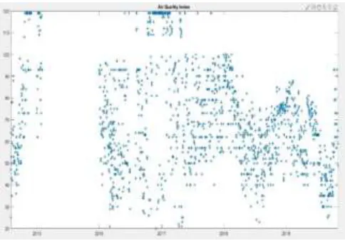
Benzene. Figure 4.1 represents the scatterplot for the concentration of air pollutants.

Fig-4.1: Scatter plot of pollutants b. DATA PRE-PROCESSING

The dataset has been found with a large number of missing entries due to sensor faults or human errors. The missing entries are filled up using median value of the data. Outliers are the data points which differs significantly with the other observationsbecause of either experimental errors or the sensory faults. This error has a serious effect in the statistical evaluation. Outlierswhich fall outside 3 standard deviations from the mean value are processed. A statistical evaluation is

replaced with clip method. Quartiles method considers above 75% data and below 25% data as an outlier. Clip method fills the detected outliers with nearest values above and below the threshold. Figure 4.2 represents the plots of various pollutants filled with median of the data for missing entries. Figure 4.3 represents the plots for various pollutants after outlier removal with the nearest threshold value.

Fig-4.3: Plots of air pollutants after removal of outliers On observing the plots in Figure 4.2 and 4.3 the data have spread accordingly on filling the missing entries and removal of the outlier. On observing the benzene data in the processed data (Fig:4.2) the authors have observed the sudden change in the data point which varied significantly compared to the other data points. Such error points are removed or clipped off in the outlier handling process. c.

d. AIR QUALITY INDEX (AQI):

(5)

Fig-4.2: Plots for pre-processed data

Fig-4.4: Calculated Air Quality Index (AQI) scatter plot

Table-1: Break Point Standards.

The equation for AQI proposed by Central Pollution Control board for individual pollutants is given by the equation-1[1].

……. (1) AQIhi = Max Aqi Range AQIlow = Min Aqi Range

Conchi = Max Break Point concentration Conclow = Min Break Point concentration Conc = Current concentration.

After Calculating the individual pollutants AQI the Overall AQI is given by the maximum of the Current day’s AQI.

i.e., AQI = Maximum (AQI_1, AQI_2, ……, AQI_n).

……… (2)

Fig-4.5: Calculated Air Quality Index (AQI)

Figure 4.5 describes the AQI calculated for the pollutant data obtained after pre-processingand outlier removal.

e.

PREDICTIVE MODELLING

Predictive modelling is a technique that uses mathematical and computational methods to forecast an event. The mathematical approach uses the equation-based phenomenon. The model parameters help how model inputs effect the output. Where the computational approach involves in the simulation to create a prediction. Regression is a statistical approach used to find the relation between the dependent and independent variables. There are different regression models in order to fit all the data into an equation.

There are total 5 types of regressions techniques are used.

i. Support vector regression ii. Decision tree regression iii. Regression Tree

iv. Gaussian Process Regression v. Linear regression

i. Support vector regression:

It is a supervised machine learning model for regression analysis. It will provide the non-linear mapping function to map a given data set M: {(x1, y1), (x2, y2) …. (xi, yi) to a high dimensional feature space. In that space a command separating hyper plane can be defined which separate the data points with maximal functional margin[3]. The algorithm involved in SVR is presented below,

AQI Category AQI Range

Break point concentration O3

(ug/m3)

NO2

(ug/m3)

PM10

(ug/m3)

PM 2.5

(ug/m3)

SO2

(ug/m3)

CO (mg/m3)

NH3

(ug/m3) Pb (ug/m3)

Good 0-50 50 40 50 30 48 1 200 0.5

Satisfactory 51-100 100 80 100 60 80 2 400 1

Moderately

Polluted 101-200 200 180 250 90 380 10 800 2

Poor 201-300 265 280 350 150 800 17 1200 3

Very Poor 301-400 748 400 430 250 1600 34 1800 3.5

(6)

Step2: Choose a kernel and its parameters as well as any regularization needed.

Step3: Form the correlation matrix, K.

Step4: Train your machine, exactly or approximately to get contraction coefficients, α = {αi}.

Step5: Use these coefficients to create your estimator, f(X, α, x*) = x*

ii. Decision Tree Regression:

It is frequently used machine learning method for regression analysis and classification. It will create a model that can target values by learning decision rules from features. If we want our response variable as categorical then that will work as a classifier, if we want our response variable as numeric then it works as a regression model.[3] The flow involved in Tree bagger is presented below,

Step1: Tree Bagger generates in bag samples by oversampling classes with large misclassification costs and under sampling classes with small misclassification costs.

Step2:consequently out of bag samples have fewer observations from classes with large misclassification costs and more observations from classes with small misclassification costs.

Step3: Tree bagger selects a random subset of predictors to use at each decision split as in the random forest algorithm. By default, tree bagger bags classification trees.

iii. Regression Tree:

Its breakdowns the data into smaller subsets while at the same time an associated decision tree is incrementally developed and represents a decision on the numerical target.it is used the examine the relation between one dependent and one independent variable. It allows input variable to be a mixture of continuous and categorial values. Regression tree is designed to approximate real-valued functions.

Step1: Regression tree breaks the data set in smaller and smaller subsets. And at the same time the associated tree will Incrementally developed. This is basically dividing the points into some groups.

Step2: The tree contains decision nodes and leaf nodes. The decision nodes are those the nodes which represent the value of input variable and it has two or more branches. The leaf nodes contain the decision or output variable. The decision node that corresponds to the best predictor becomes the top most node called the root node.

Step3: The algorithm decides the optimal number of splits and splits the dataset accordingly.

Fig: 4.6: Plot of Regression Tree

Figure 4.6 shows the regression tree model with the pruning level of 75 out of 126 levels.

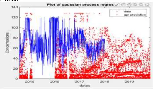
Gaussian process generates data located throughout some domain such that any finite subset of range follows a multivariate gaussian distribution. It is a interpolation method for which the interpolated values are modelled by a gaussian process governed by prior covariance. The prior covariance is specified by passing a kernel object. The procedure involved in GPR is shown below,

Step1: Assume a Gaussian process prior which can be specified using a mean function and covariance function. Step2: Calculate the probability distribution over all admissible functions that fit the data.

Step3: Calculate the posterior using the training data, and compute the predictive posterior distribution on our points of interest.

Fig-4.7: Gaussian Process Regression v. Linear Regression:

Linear Regression is used to find the relationship between one or more multiple inputs x and one output y. [3]

Step1: Start with a training set

X is input training data Y labels the data

When training the model – it fits the best line to predict the value of y for a given value of x. The model gets thebest regression fit line by finding the best θ1 and

θ2 values.

Step2: Start with parameter with random variables.

Step3:The algorithm learns the line, plane or hyper-plane that best fits the training sample

Step4: Prediction: uses the learning line, plane or hyper-plane to predict the output value for any input sample.

Artificial Neural Network:

(7)

Step1: Initialising the training epoch =1

Step2:Initialising network of weights and biases with uniform distribution values

Step3: Calculate actual output of actual units and hidden units Step4: Calculate error.

Fig 4.8: Neural network layers

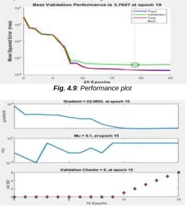
The performance plot and the train state plots for the neural network algorithm that used for training a model, Levenberg-Marquardt is as shown below in figure 4.9

Fig. 4.9: Performance plot

Fig.4.10: Training State Plot.

In this Model we set the Target as AQI and all the other parameters like PM10, PM2.5, O3, etc. as the input vector. For employing the regression model to the data set, the data splitsinto two partitions. The first one is for training the model and other set for testing. Data before Jan-2019 for training and after Jan-2019 for testing the model. The Quality metrics or performance features like Mean Square Error, Mean Absolute Error, Root Mean Square Error, R squared Error, Median error, Median absolute error, Average error etc. were

computed.The Quality Metrics for different models are tabulated in table-3. Evaluation of each model is done to estimate the performancefor forecasting.

MAE: Mean Absolute Error is the difference between the original and the forecasted values extracted by averaged the absolute difference over the data.[10][14]

∑

MSE: Mean Square Error is the difference between the original and the forecasted values extracted by square of the difference over the data.[10][14]. MSE is the averaged square per prediction.[15]

∑

R-Squared: Coefficient of determination, represents the coefficient of how better the values fit compared to the original values.[10]

∑

RMSE: The square root of the difference between the original and forecasted values extracted by the square of the difference over the data.[10]

√

√ ∑

Where Yi is the current value in Y

Y’ is the predicted value of Y Y’’ is the mean value of the Y.

(8)

Fig-4.11: Test Set using different regression models.

In figure 4.11 represents the final plots of actual versus predicted using different regression models like SVR, GPR LR, etc, and Neural Networks applying the Levenberg- Marquardt training algorithm.

5. CONCLUSION & FUTURE SCOPE

Different regression modelsand Neural Networksare used for predicting the AQI using the previous data of the Vijayawada City. The AQI value for the test set year 2019 hasbeen forecasted with the different regression models and the Neural Networks. Support vector machine-based regression

model has provided MSE of 98.431 and R2 error of 0.599. Gaussian process regression-based model has provided MSE of 10.355and R2 error of 0.958. Linear regression model has provided MSE of 61.302and R2 error of 0.750. Tree regression model has provided MSE of 0.744and R2 error of 0.997.Tree bagger-based regression model has provided

(9)

MSE of 11.747and R2 error of 0.952. Neural Network has provided the MSE of 0.857 and R2error of 0.997. Neural network and regression tree have provided same R2 error. Tree regression model gives lowest MSE. Tree regression model provides better performance when compared to all other models in terms of MSE and R2 error. Deep learning can be employed to learn features of pollutants and may provide better classification.

ACKNOWLEDGEMENT

The authors acknowledge theauthorities of Andhra Pradesh Pollution Control Board - Vijayawada forproviding with necessary air pollution data.Authors thank their parents, teachers for their constant help and support. Authors extend theirthanks to the director, Andhra Loyola Institute of Engineering and Technology, Vijayawada, Dr. Francis Xavier SJ, Principal of the institute, members of Dr.APJ Abdul kalam research forum, staff of the department of ECE for their constant inspiration and encouragement.

REFERENCES

[1]. Control of urban Pollution series CUPS/ 82/2014-2015 “National Air Quality Index” Central Pollution Control Board, Ministry of Environment Forest and Climate Change.

[2]. Chavi Srivastha, Shyamli Singh, Amit Prakash Singh:’ Estimation of Air Pollution in Delhi using Machine Learning Techniques’,2018 International Conference of Computing, Power and Communication Technologies(GUCON).

[3]. Ka Hu, Ashfaqur Rahman, Vijay Sivaraman: ‘HazeEst: Machine Learning Based Metropolitan Air PollutionEstimation from Fixed and Mobile Sensors’, DOI10.1109/JSEN.2017.2690975 IEEE Sensors journal. [4] Aditya CR, Chandana R Deshmukh, Nayana D K,

PraveenGandhi:’ Detecting and Prediction of Air Pollution UsingMachine Learning Models’, International Journal of Engineering Trends and Technology (IJETT)-volume 59 issue /24-May 2018.

[5]. Sachit Mahajan, Ling-Jyh Chen, Tzu-Chieh Tsai: AnEmpirical Study of PM2.5 Forecasting Using neuralnetwork. IEEE Smart World Congress, At San Francisco,USA 2017.

[6]. Jan Kleine Deters, Rasa Zalakeviciute, Mario Onzalez, Yves Rybarczyk:’Modelling PM2.5 Urban Pollution Using Machine Learning and Selected Meteorological Parameters’ Hindawi, journal of Electrical and Computer Engineering,Volume 2017, Article ID 5106045.

[7].V.Duc Le, Sang Kyun Cha, ‘Real-time Air Pollution prediction model based on Spatiotemporal Big data’.The International Conference on Big data, IoT, and Cloud Computing (BIC 2018)

[8]. Ping Wang a, Yong Liua, Zuodong Qin a, Guisheng Zhang b,’ A novel hybrid forecasting model for PM10 and SO2 daily concentrations’ Science of the Total Environment 505 (2015) 1202–1212.

[9]. Sachin Bhogtie, Sejal Pitale, Pooja Bhalgat’ Air Quality Prediction Using Machine Learning Algorithms’, Internationl Journals of Computer Applications Technology and Research Volume 8-Issue 09,367-370,2019, ISSN: -2319-8656.

[10].Ping Wang a, Yong Liua, Zuodong Qin a, Guisheng Zhang b,’ A novel hybrid forecasting modelforPM10andSO2 daily concentrations’Science of the Total Environment 505 (2015) 1202–1212.

[11]. Z. Qi and et al., “Deep Air Learning: Interpolation, Prediction, and Feature Analysis of Fine-grained Air Quality,” TKDE 2018, IEEE transaction on knowledge anddata engineering vol.30 no.12.

[12].Azman azid, HafizanJuahir, Mohd Khairul Amri Kamaruddin, Ahmad Shakir MohdSoudi,” Prediction of the level of Air pollution using principle component analysis and artificial neural network techniques: a case study in Malaysia”, Water Air Soil pollut(2014) 225:2063, DOI: 10.1007/s 11270-014-2063-1

[13]. Norusis, M.J. (1990). SPSS base system user’s guide. Chicago, IL, USA: SPSS.

[14].Shikha Saxena, Anil K Mathur, ‘Prediction of Respirable Particulate Matter (PM10) Concentration using Artificial Neural Network in Kota city’, Asian Journal of Convergence in Technology Volume III, Issue III ISSN No.:2350-1146, I.F-2.71.