NOVEL SECOND-ORDER TECHNIQUES AND GLOBAL
OPTIMISATION METHODS FOR SUPERVISED TRAINING
OF MULTI-LAYER PERCEPTRONS
Adrian John Shepherd
Thesis submitted for the degree of
Doctor o f Philosophy in the University o f London
September 1995
ProQuest Number: 10106017
All rights reserved
INFORMATION TO ALL USERS
The quality of this reproduction is dependent upon the quality of the copy submitted.
In the unlikely event that the author did not send a complete manuscript and there are missing pages, these will be noted. Also, if material had to be removed,
a note will indicate the deletion.
uest.
ProQuest 10106017
Published by ProQuest LLC(2016). Copyright of the Dissertation is held by the Author.
All rights reserved.
This work is protected against unauthorized copying under Title 17, United States Code. Microform Edition © ProQuest LLC.
ProQuest LLC
789 East Eisenhower Parkway P.O. Box 1346
ABSTRACT
Conventional training methods for multi-layer perceptrons (MLPs), derived from the traditional backpropagation algorithm, have three serious inadequacies: convergence to a solution is frequently slow; they do not always converge to the desired global solution; and their performance is highly dependent on the setting of one or more user-defined parameters. A growing body of research indicates that second-order training methods, derived from classical optimisation theory, offer substantial improvements in training speed and a reduced sensitivity to initial parameter settings. However, experiments
conducted for this research suggest that most second-order methods have worse global convergence properties than conventional methods. On the other hand, training methods that are designed to have better global convergence characteristics than conventional methods - for example, stochastic training methods - are typically as slow or slower than conventional methods.
The aim of this research is to develop MLP training algorithms that are both fast and globally-reliable' by combining second-order methods with a novel deterministic strategy for global optimisation. Expanded Range Approximation (ERA). Unlike most stochastic methods for global optimisation, the implementation of ERA with a second-order algorithm is trivial. When tested on benchmark training tasks, hybrid second-order/ERA algorithms (with appropriate parameter settings) were considerably faster and converged to a global minimum as or more frequently than conventional algorithms.
CONTENTS
Acknowledgements 6
List of Figures 7
List of Graphs 8
List of Tables 10
1. INTRODUCTION
11
2. MULTI-LAYER PERCEPTRON TRAINING
13
2.1 Introduction to MLPs 13
2.1.1 The MLP architecture 13
2.1.2 MLP training 15
2.2 Error Surfaces and Local Minima 17
2.2.1 The MLP error surface 17
2.2.2 Local minima 19
2.3 Backpropagation 20
2.3.1 Backpropagation - an overview 20
2.3.2 On-line backpropagation 22
2.3.3 Backpropagation with momentum 24
3. CLASSICAL OPTIMISATION
25
3.1 Introduction to Classical Methods 25
3.1.1 The linear model and steepest descent 26
3.1.2 The quadratic model and Newton’s method 28
3.1.3 Line-search methods vs. model-trust region methods 30
3.1.4 Special methods for nonlinear least squares 32
3.1.5 Scaling and preconditioning 34
3.2 Line Minimisation 36
3.2.1 Line minimisation strategies 36
3.2.2 Safeguarded polynomial interpolation 37
3.2.3 Inaccurate line searches 38
3.2.4 Backtracking line search 39
3.2.5 Hybrid Brent/backtracking line search 40
3.2.6 Line search implementation 41
3.3 Model-Trust Region Strategies 41
3.3.1 A simple model-trust region algorithm 41
3.3.3 Modem model-tmst region algorithms 43
3.4 Quasi-Newton Methods 44
3.4.1 The Hessian update formula 44
3.4.2 Representing the Hessian approximation matrix 45
3.4.3 Modified quasi-Newton methods 46
3.5 Conjugate Gradient Methods 47
3.5.1 The conjugate gradient formula 47
3.5.2 Conjugate gradient restarts 48
3.6 Levenberg-Marquardt Method 49
3.6.1 From Gauss-Newton to Levenberg-Marquardt 49
3.6.2 Neural implementation 50
3.7 Comparison of Methods 51
4. CLASSICAL MLP TRAINING METHODS
52
4.1 Research Review 52
4.2 Benchmark Training Sets 60
4.2.1 Benchmark criteria 60
4.2.2 XOR 61
4.2.3 The sine problem 63
4.3 Experimental Results 64
4.3.1 General training conditions 64
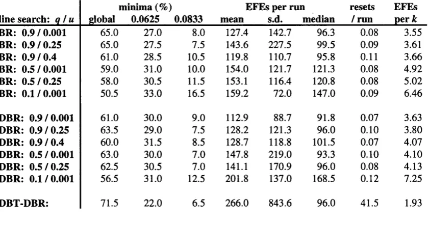
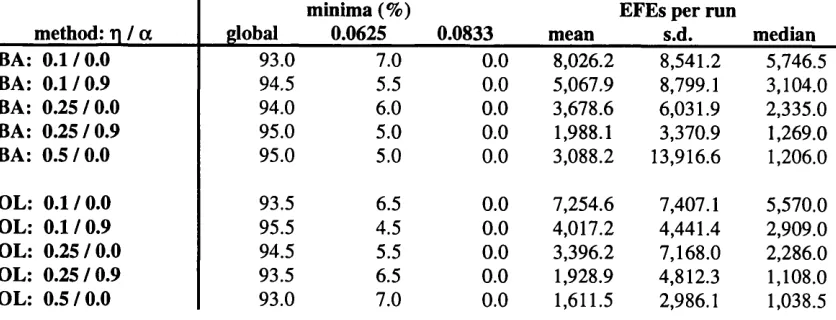
4.3.2 XOR results, sigmoid output nodes 69
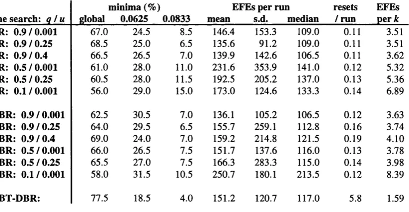
4.3.3 XOR results, linear output nodes 74
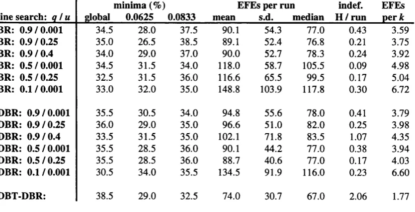
4.3.4 Sine results 80
4.4 Comparison of Training Methods 85
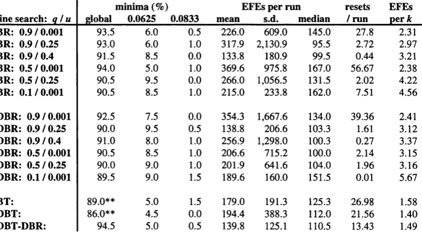
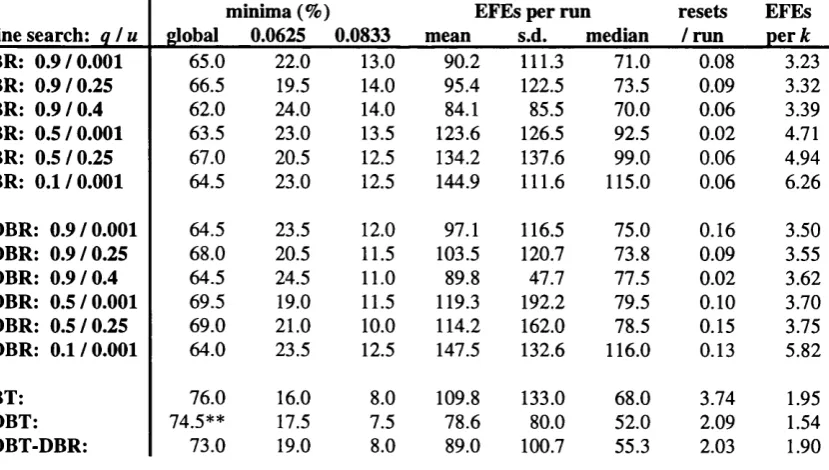
4.4.1 Convergence to local minima 85
4.4.2 Training speed and accuracy 95
4.4.3 Conclusion 111
5. GLOBAL OPTIMISATION - A NEW ERA?
112
5.1 Introduction to Global Optimisation 112
5.1.1 Stochastic methods 112
5.1.2 Deterministic methods 117
5.2 Expanded Range Approximation (ERA) 118
5.2.1 Introduction 118
5.2.2 How ERA works 120
5.2.3 Implementing ERA 125
5.3 Conclusion 141
6. CONCLUSION
142
ACKNOWLEDGEMENTS
The British postgraduate student is a lonely forlorn soul... for whom nothing has been real since the Big Push.
David Lodge*, Changing Places
I would like to thank the following for making this thesis possible, and for saving me from the narrow existence of the British postgraduate student':
• my first-supervisor. Dr Denise Gorse, for her enthusiastic guidance throughout the production of this thesis;
• my second-supervisor. Dr Simon Arridge, for sharing his knowledge and experience in the field of classical optimisation;
• Templer Hart, for the generous gift of computer equipment, and for acting as an unpaid PC help-desk operator;
LIST OF FIGURES
Figure 1 Minimal 2-2-1 MLP architecture, suitable for learning the XOR
problem_____________________________________________________ 14 Figure 2 Steepest descent and the ‘narrow valley effect' __________________ 27 Figure 3 Parameter u and the model-tmst region search direction___________ 32 Figure 4 Schematic representation of error surfaces E(0) (with a single
global minimum) and E] (with multiple minima)____________________ 123 Figure 5 Illustration of how the number of stationary points in error surface
E(t|) is determined by the size of r| (T|,<T)2<T|3). Stationary points in
LIST OF GRAPHS
Graph 1 Sample location of XOR stationary points in terms of pattern
classification/misclassification___________________________________ 62 Graph 2 Location of sine stationary points in terms of pattern
classification/misclassification___________________________________ 64 Graph 3 Training algorithm convergence to global minima (XOR, sigmoid) 86 Graph 4 Training algorithm convergence to global minima (XOR, linear) ____ 86 Graph 5 Training algorithm convergence to global minima (sine)___________ 87 Graph 6 Global convergence frequency vs. log mean resets per successful run,
QN line-search methods (XOR, sigmoid)___________________________ 90 Graph 7 Line searches and global convergence (XOR, sigmoid)____________ 92 Graph 8 Line searches and global convergence (XOR, linear)______________ 92 Graph 9 Model-trust region strategies and global convergence (XOR, sigmoid)
___________________________________________________________ 94 Graph 10 Relative frequency histogram, SD DBR: 0.5 / 0.25 (sine)_________ 96 Graph 11 Training speed, first- and second-order methods (XOR, sigmoid)___ 97 Graph 12 Training speed, first- and second-order methods (XOR, linear)____ 97 Graph 13 Training speed, first- and second-order methods (sine)___________ 98 Graph 14 Training speed, second-order methods (XOR, sigmoid)___________ 99 Graph 15 Training speed, second-order methods (XOR, linear) ___________ 100 Graph 16 Training speed, second-order methods (sine)__________________ 100 Graph 17 Training speed, PR CO with SD resets (XOR, sigmoid)_________102 Graph 18 Training speed, PR CO with SD resets (XOR, linear)___________102 Graph 19 Training speed, PR CG with SD resets (sine) _________________103 Graph 20 Training speed, NQN with SD resets (XOR, sigmoid)___________ 103 Graph 21 Training speed, NQN with SD resets (XOR, linear)____________ 104 Graph 22 Training speed, NQN with SD resets (sine)___________________ 104 Graph 23 Training speed, QN with SD resets (XOR, sigmoid) ___________105 Graph 24 Training speed, QN with SD resets (XOR, linear)______________105 Graph 25 Training speed, QN with SD resets (sine)____________________106 Graph 26 Training speed, QN without resets (XOR, sigmoid)____________106 Graph 27 Training speed, QN without resets (XOR, linear)______________107 Graph 28 Training speed, QN without resets (sine)_____________________107 Graph 29 EFEs per run vs. EFEs per epoch, QN methods without resets
(XOR, sigmoid)_____________________________________________ 109 Graph 30 EFEs per run vs. EFEs per epoch, QN methods without resets
(XOR, linear)_______________________________________________ 110 Graph 31 EFEs per run vs. EFEs per epoch, QN methods without resets
(sine)______________________________________________________ 110 Graph 32 N-sX&p ERA, global convergence frequency vs. log N
(XOR, sigmoid)_____________________________________________ 129 Graph 33 A-step ERA, global convergence frequency vs. log N
(XOR, linear)_______________________________________________ 130 Graph 34 Sample 10-step ERA training curve, QN without resets
Graph 35 Trajectory of network outputs for XOR patterns 00 and 10
with T)=l___________________________________________________ 133 Graph 36 Trajectory of network outputs for XOR patterns 00 and 10
with T|=0.3_________________________________________________ 134 Graph 37 Trajectory of network outputs for XOR patterns 00 and 10
with T|=0.2_________________________________________________ 135 Graph 38 Trajectory of network outputs for XOR patterns 00 and 10
with T|=0.1 _________________________________________________ 136 Graph 39 The value of a single MLP weight plotted as a function of time
LIST OF TABLES
Table 1 69
Table 2 69
Table 3 70
Table 4 70
Table 5 71
Table 6 71
Table 7 72
Table 8 72
Table 9 73
Table 10 73
Table 11 74
Table 12 74
Table 13 75
Table 14 75
Table 15 76
Table 16 76
Table 17 77
Table 18 77
Table 19 78
Table 20 78
Table 21 79
Table 22 79
Table 23 80
Table 24 80
Table 25 81
Table 26 81
Table 27 82
Table 28 82
Table 29 83
Table 30 83
Table 31 84
Table 32 84
Table 33 mean resets bv E=0.0625 tXOR. sigmoidl 88
Table 34 mean resets by E=0.0625 tXOR. linear! 88
Table 35 mean resets bv E=0.0625 tsine! 88
Table 36 mean resets by E=0.0625. QN methods 89
Table 37 MLP architectures, training set sizes, and numbers of runs used
in testing the proposition that E(0) has only a global minimum 121
Table 38 A^-step ERA. XOR with sigmoid output nodes 127
Table 39 N-step ERA. XOR with linear output nodes 128
Table 40 A^-step ERA. sine task 129
Table 41 ERA expansion-rate parameter. P 138
1. INTRODUCTION
Conventional training methods for multi-layer perceptrons (MLPs), derived from the traditional backpropagation algorithm, have three serious inadequacies: convergence to a solution is frequently slow; they do not always succeed in converging to a desired (and achievable) solution, irrespective of the number of training iterations allowed; and they tend to be highly sensitive to the choice of input-parameters, set heuristically by the user. A growing body of research (reviewed in section 4.1) indicates that second-order training methods, derived from classical optimisation theory, offer substantial improvements in training speed as well as a greatly reduced sensitivity to the choice of initial parameters. However, experiments conducted for this research suggest that most second-order methods have worse global convergence properties than conventional methods; tested on benchmark tests with known local minima, second-order methods failed to converge to the desired global solution as frequently as conventional methods. On the other hand, training methods that are designed to have better global convergence characteristics than
conventional training methods - for example, stochastic training methods - are typically as slow or slower than conventional algorithms.
The underlying aim of this research is the development of MLP training algorithms that are both faster and more globally-reliable' than conventional training methods. The approach adopted here has been to combine fast second-order classical algorithms with a novel deterministic strategy for global optimisation - Expanded Range Approximation, or ERA for short. When tested on benchmark tasks, hybrid second-order/ERA training algorithms (with appropriate parameter settings) were considerably faster and converged to a global minimum as or more frequently than conventional training algorithms.
2. MULTI-LAYER PERCEPTRON TRAINING
The class of neural network considered in this research is the multi-layer perceptron (MLP)’ . MLPs have a wide range of applications, including pattern classification and function-learning [Lisboa, ed., 1992]. MLP training involves adjusting the network so that it is able to produce a specified output for each of a given set of input patterns; since the desired outputs are known in advance, MLP training is an example of supervised
learning.
This chapter sets the context for the research presented in the remainder of this thesis: section 2.1 considers the physical properties and dynamics of MLP training, section 2.2 the essential characteristics of MLP training tasks and their implications for training algorithm design, and section 2.3 the properties of error-backpropagation, the dominant training paradigm for MLPs.
2.1 Introduction to MLPs
2.1.1 The M LP architecture
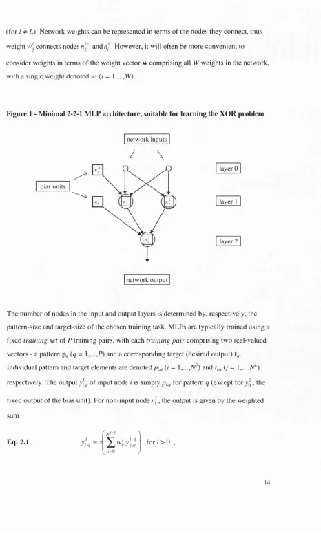
The MLP architecture consists of units or nodes arranged in two or more layers. (The input layer, which serves only to distribute the input from each pattern, is not counted.) Some of the nodes are connected by real-valued weights, but there are no connections between nodes in the same layer. For notational convenience, it is assumed throughout that MLP architectures are of a ‘standard’ form, with adjacent layers fully-connected but no connections between non-adjacent layers. Such an MLP consists of L layers with nodes in each layer (/ = 0,...,L), with I = 0 denoting the input layer. The notation for a
single node is n' (i = 1,...,V). The thresholds for the weighted sum of inputs to each node
(given by Eq. 2.1 below) are treated uniformly by adding an extra node with a fixed
output of 1.0 to all but the output layer. This node - called the bias unit - is denoted
(for / ^ L). Network weights can be represented in terms of the nodes they connect, thus
weight w\j connects nodes n~^ and n \. However, it will often be more convenient to
consider weights in terms of the weight vector w comprising all weights in the network, with a single weight denoted w, (/ = l,...,Vk).
Figure 1 - Minimal 2-2-1 MLP architecture, suitable for learning the XOR problem
bias units
network inputs
/
\
network output
layer 0
layer 1
layer 2
The number of nodes in the input and output layers is determined by, respectively, the pattern-size and target-size of the chosen training task. MLPs are typically trained using a fixed training set of P training pairs, with each training pair comprising two real-valued vectors - a pattern (^ = 1 and a corresponding target (desired output)
Individual pattern and target elements are denoted (/ = 1 ,...,A^) and tj,^ (j = 1 ,...,N^)
respectively. The output of input node i is simply p ^ for pattern q (except for y j , the
fixed output of the bias unit). For non-input noden/, the output is given by the weighted
sum
Eq. 2.1
M,y'u
7 =0
where the activation or squashing function s is typically the sigmoid:
1
Eq. 2.2 =
1 + e'
The layers between the input and output layers are known as hidden layers. The number of hidden layers and nodes has a major impact on MLP training: too few, and the network will be unable to learn the problem; too many, and the network may take excessively long to train and have poor generalisation capabilities - a measure of the network’s ability to classify patterns which share the same general features as, but are not identical to, patterns in the training set. Numerous schemes have been developed which calculate an appropriate number of hidden nodes from the training data or which adapt the architecture (i.e. add or ‘prune’ nodes) during training [Brent, 1991] [Hirose, Yamashita & Hijiya, 1991] [Santini, 1992]. (Upper and lower bounds on the number of nodes are given in [Huang & Huang, 1991].) None of these schemes have been adopted for this research, since the appropriate architecture was known in advance for the chosen benchmark tests, but all the training methods presented here could easily be modified to incorporate such schemes.
2.1.2 M LP training
MLP training is an iterative process which involves, at each iteration or epoch, the calculation of network outputs for each pattern in the training set and the adjustment of network weights according to the disparity between actual and desired outputs. Prior to training, the weights are initialised to small random values - small to prevent saturation (where one or more hidden nodes is highly active or inactive for all patterns and therefore insensitive to the training process) and random to break symmetry. The choice of
initialisation range can have a significant impact on training performance (see [Kolen & Pollack, 1990]).
;=1
The advantages of Eq. 2.3 are consistency with the majority of MLP research and compatibility with the nonlinear least squares methods considered in sections 3.1.4 and 3.6. However, the MSB function is a ‘greedy’ error function; the number of
misclassifications can increase from one iteration to the next despite a reduction in E. Other error functions, such as the exponential, frequently perform better in practice [M0ller, 1993e, 65-70 & 149-161]. An investigation of the impact of different error functions on the training methods presented here will be the subject of future research.
MLP training is deemed to be successful when E becomes ‘acceptably’ small. Precisely how small is application-specific, but a close approximation to zero is generally undesirable since an MLP’s ability to generahse decreases with overtraining [Hecht- Nielsen, 1990, 116].
The key factor in the dynamics of MLP training is the role of the hidden nodes. A hidden node that duplicates the function of another hidden node is redundant, i.e. makes no useful contribution to the training process. A mathematical analysis by Annema et al. of the dynamics of MLP training indicates that the build-up and dissipation of hidden-node redundancy is an integral part of the training process [Annema, Hoen & Wallinga, 1994]. The core analysis, which holds for a two-layer MLP with two hidden nodes and ‘very small’ initial weights, describes three distinct training phases; for MLPs of arbitrary size, this three-phase analysis can be applied iteratively to smaller and smaller clusters of redundant hidden nodes.
vectors associated with each cluster now converge towards different attractors in weight space.
The inability of an MLP to ehminate hidden-node redundancy (i.e. to proceed beyond phase two of the preceding analysis) is a frequent cause of training failure (see section
2.2.1).
2.2 Error Surfaces and Local Minima
In order to design efficient and reliable training algorithms, it is essential to gain an understanding of the principal characteristics of MLP training tasks and their implications for different training strategies. The perspective adopted here is that of function
optimisation - that is, the minimisation of the MLP error function E. Viewed in these terms, MLP training is an error-minimisation or optimisation process (for which many techniques have been developed outside the neural network field), and each training task defines a multi-dimensional non-negative error surface (section 2.2.1), formed by plotting the value of E for all (reasonable) settings of the MLP weight vector w. This approach has two important benefits: it aids visualisation of the training process through analogy with a three-dimensional landscape; and it leads to numerically-testable definitions for many of the conditions encountered during training.
The lowest points on the error surface are known as global minima. (Typically MLP error surfaces have multiple global minima, each of which is a surface rather than a single point.) If the lowest point of a ‘basin’ in the error surface has a higher error than that associated with a global minimum, it is termed a local minimum. Since the impact of local minima on MLP training is a major theme of this research, they are considered separately in section 2.2.2.
2.2.1 The M LP error surface
weights. The precise shape of the error surface is problem- and architecture-specific; since it is impractical to produce a map of an error surface that is both detailed and extensive (even for small training problems and architectures), it is no surprise that the properties of MLP error surfaces remains a subject for debate [Hecht-Nielsen, 1990,
131].
It is worth stressing that the common practice of inferring the presence of landscape features based on training error-curve information alone is highly suspect. There is, for example, a tendency to say an MLP has become trapped in a local minimum whenever the training curve flattens out at a comparatively high level, despite the fact that there are equally plausible causes for this behaviour which are unrelated to local minima. This is not simply a case of pedantry about the use of terminology; the precise cause of a given training characteristic may have profound implications for the efficacy of an attempted solution.
What reliable evidence there is (for example, from contour plots of small sections of an error surface) suggests that most MLP error surfaces share a number of broad
characteristics: a high degree of smoothness', 'a multitude of areas with shallow slopes in multiple dimensions simultaneously' [Hecht-Nielsen, 1990,131] (‘plateaus’);
convolutions and ellipses of high eccentricity (‘valleys’); and many ‘basins’ or minima. MLP error surfaces typically have multiple global minima, owing to permutations of the weights that leave the MLP input-output function unchanged; an assessment of the prevalence of local minima is deferred to section 2.2.2.
‘Plateaus’, ‘narrow valleys’, and local minima often prove to be serious obstacles to successful training. If an MLP encounters a region with very shallow gradients, it can take many training epochs before a significant reduction in E is made - the network is said to be stuck in a temporary minimum [Annema, Hoen & Wallinga, 1994]. Training algorithms derived from the steepest descent method are prone to slow training in narrow valleys (see section 3.1.1). And algorithms which do not allow an increase in E at any epoch are prone to becoming trapped in local minima, i.e. no amount of additional
three most frequently encountered are redundant hidden nodes, hidden node saturation, and ‘dead regions’ of weights space where all hidden nodes are inactive [Wessels, Barnard & van Rooyen, 1990].)
The characteristics of MLP error surfaces give a good indication of the kinds of strategy that are likely to engender efficient and reliable training: the smoothness of the error surface suggests that classical optimisation with derivatives (chapters 3 and 4) will be effective; rounding errors, floating-point precision and the choice of termination criteria are likely to be important in nearly flat regions; some methods are far less prone to slow progress in ‘narrow valleys’ than others; and, if there are local minima, global
minimisation strategies (chapter 5) may be necessary to ensure an acceptable probability of training success.
2.2.2 Local minima
For the purposes of this research, the term ‘local minimum’ is used in a rigorous
mathematical sense. If, for a given combination of MLP architecture and training task, the error function E(w) is twice-continuously differentiable (i.e. the second-derivatives of E are continuous), it is possible to define useful theoretical conditions for a point w* to be a minimum of E in terms of the gradient vector g(w*)
Eq.2.4
dw-and Hessian matrix G(w*)
a"E (w )
Eq. 2.5 G, =
^ dW;dw;
< J
If g(w*) is zero, w* is a stationary point - which means it is either a minimum, a
maximum or a saddle point. Stationary point w* is definitely a minimum if G(w*) is positive definite (i.e. all the eigenvalues of G are strictly positive), and may be a minimum if G(w*) is positive semi-definite (i.e. all the eigenvalues of G are non
The prevalence of local minima in MLP error surfaces remains a matter of debate. Local minima are known to occur with specific test problems [Mclnemey et al., 1989] [Lisboa & Perantonis, 1991]. On the other hand, local minima cannot occur if the training task is linearly separable [Gori & Tesi, 1992], if there are as many hidden nodes as patterns in
the training set [Poston et al., 1991], or if the number of patterns is less than or equal the
number of pattern elements [Yu, 1992] - assuming, in each of these cases, that the chosen architecture is capable (with some set of weights) of learning the task in question.
Unfortunately, none of these results give much guidance to real-world applications, for which there is precious little hard evidence on either side of the debate. At present, it is probably reasonable to conclude that for many (if not all) realistic applications local minima present a serious obstacle to successful training.
Every minimum has an associated basin o f attraction - a region surrounding the minimum from which it is only possible to escape by passing over higher ground (or by deforming the error surface in some way). A number of contrasting approaches have been proposed for reducing the likelihood of an MLP getting trapped in the attractive basin of a local minimum, including: stochastic methods (section 5.1.1); deterministic strategies, such as homotopic methods (section 5.1.2); changing the error function [Solla, Levin & Fleisher, 1988]; weight initialisation schemes [Wessels & Barnard, 1992]; and schemes for dynamically changing the number of hidden nodes [Hirose, Yamashita & Hijiya, 1991]. As these schemes apply to different aspects of the training process, it is likely that the ‘optimal’ strategy will combine several of these schemes in a single algorithm.
2.3 Backpropagation
2.3.1 Backpropagation - an overview
The vast majority of MLP research has used a version of the backpropagation (BP) training method (rediscovered and disseminated to a wide audience by [Rumelhart, Hinton
In essence, BP implements gradient or steepest descent (section 3.1.1) for an MLP. At each epoch k the gradient g(wt) is calculated and the weights updated according to the
simple rule
Eq. 2.6 - n S t , fo rrj> 0 ,
where T) is a constant heuristically-chosen training rate, typically set in the range [0, 1]. A reduction in total network error E at each epoch is guaranteed so long as the gradient is
greater than zero and T) is sufficiently small. The calculation of the gradient by backpropagation is implemented in two phases - a forward pass and a backward pass. 'Yïie, forward pass generates the network outputs for pattern p through the calculation of
each y \ p, from layer / = 1 to / = L, according to the weighted sum of Eq. 2.1. The
backward pass calculates the partial contribution of pattern p to the total network
error E, and the corresponding partial gradient with elements . These
elements are calculated by applying the following rule from layer / = L to / = 1 :
Eq.2.7 a £ ,/a w ' = 5 ',y ': ; ,
where the error term ô is given by
Eq.2.8 K p = [ h .p - y t p ) y i .p { ^ - y l)
K . P = y '> . p {^ -y ] . p ) lL K p < '^ f ° ^ i< i^ ■ (=1
A single training epoch consisting of P forward passes interleaved with P backward passes.
updates, the adaptation of the MLP training rate, and the addition of noise to the weights. All these techniques have reported strengths when applied to specific problems, but tend to be ineffective in general. Moreover, many require an additional problem-specific parameter (or parameters) to be set heuristically by the user.
One implication of this diversity of practical BP implementations is that the choice of a ‘fair’ BP benchmark is extremely difficult. This thesis considers only two of the most widely-used modifications to the standard BP algorithm - on-line training (section 2.3.2) and momentum (section 2.3.3). The steepest descent algorithm, a 'classical'
implementation of batch BP that sets the training rate optimally at each epoch, is described in section 3.1.1.
2.3.2 On-line backpropagation
On-line BP^ differs from batch BP in that the weights are updated at the end of each
backward pass (i.e. P times per epoch), rather than once every P backward passes (i.e. once per epoch). The weight update rule for on-line BP is
E q .2.9 = w J-T ig * , forTi>0.
Typically, the P patterns are presented to the network in random order. If the training rate
Tj tends to zero, on-line BP can be regarded as an approximation to batch BP; however,
for practical settings of r| the two methods diverge.
In theory, on-line BP has several potential disadvantages compared to batch BP:
• it is not guaranteed to 'make progress' (i.e. reduce E) at each training epoch;
• it requires slightly more computational effort per epoch than batch BP;
• the optimal training rate for on-line BP is poorly understood (cf. the batch mode steepest descent method);
• it is much more difficult to analyse.
Nevertheless, on-line BP has several practical advantages over batch BP:
• on-line BP is an example of a stochastic process that can prevent an MLP
from getting trapped in a local minimum;
• if the training set contains redundant information, the more frequent weight updates of on-line BP often prove more efficient [M0ller, 1993b] (although it may be possible to remove redundant information by pre-processing the training set [Battiti, 1992]);
• on-line training is essential if the full complement of training patterns is not known at the start of training.
For these reasons, on-line BP can be regarded as the backpropagation benchmark.
There are two ways in which on-line BP can be regarded as a stochastic process. Firstly, the total network error E may rise at one or more epochs such that the network is able to escape from the basin of attraction of a local minimum. Secondly, the shape of the MLP error surface is not constant with on-line BP; local minima are meta-stable states which
slowly decay to the global minimum, at a rate of t jt for some constant t that is 'much
larger than the typical time scale \jt to reach equilibrium inside an attractive region'
[Kappen & Heskes, 1992,72]. In its traditional' form - with weights updated after the presentation of every pattern - on-line BP makes no attempt to regulate the amount of stochastic 'noise' added to the system at each training epoch. However, the term 'on-line training' is often used in a more general sense to encompass training algorithms which
2.3.3 Backpropagation with momentum
Backpropagation with momentum uses a modified version of the standard BP weight update formula (given by Eq. 2.6), as follows:
Eq. 2.10 = -T|gt + cxAw^, for Tj > 0 and 0 < a < 1 ,
where a is known as the momentum term. (With momentum turned 'off, i.e. with a=0, Eq. 2.10 is equivalent to the standard update of Eq. 2.6.) Experience shows that the addition of momentum can significantly speed up the BP training algorithm, attributable to its impact in precisely those regions of the MLP error surface where the
backpropagation algorithm performs badly - 'plateaus' and 'narrow valleys'; the
momentum term accelerates convergence in flat regions by a factor that approaches ^ 1 - a as the number of epochs (k) gets large, and reduces the number of oscillations in a narrow valley - i.e. reduces the 'narrow valley effect' (see section 3.1.1) - by averaging out the components of the gradient which alternate in sign [Watrous, 1987]. As M0ller points out [1993e, 19], batch BP with momentum can be viewed as an approximation to conjugate gradient methods (section 3.5) - the important difference being that conjugate gradient methods chose parameters Tj and a automatically at each iteration, whereas batch BP with momentum sets T[ and a to fixed heuristic values.
An alternative weight update to Eq. 2.10, given by
Eq. 2.11 Awjt+, = - ( l - a ) r |g ^ + a A w ^ , fo rt| > 0 and 0 < a < 1,
3. CLASSICAL OPTIMISATION
3.1 Introduction to Classical Methods
Unconstrained nonlinear optimisation is a mature branch of numerical analysis
concerned with the minimisation of multi-dimensional functions^. For a wide class of smooth convex functions, convergence is guaranteed. However, classical optimisation is concerned only with local optimisation.
All the optimisation methods considered in this chapter share important characteristics: all derive, algebraically, from the Taylor-series expansion of a smooth function / i n the neighbourhood of an arbitrary point x
Eq. 3.1 f(x-l-s)= f(x )-l-g (x )^s+ is^ G(x)s+... ;
all are iterative descent algorithms (i.e. minimum x* is located in a series of steps, with
f(xjt+i) < f(xjfe) at each step); and all are hybrid methods, which fall somewhere between the steepest descent method (section 3.1.1) and Newton’s method (section 3.1.2).
In order to compare the theoretical performance of these methods, it will be useful to consider their global and local convergence properties. In the context of the convergence of classical algorithms, the terms ‘local’ and ‘global’ have a different meaning to that introduced in section 2.2. A method is said to be globally convergent if, for an arbitrary smooth convex function, it is guaranteed to converge (eventually) to a minimum from (almost) any starting position. (The global convergence properties of algorithms
associated with convex functions are applicable to non-convex functions inside the basin of attraction of a minimum.) A method’s local convergence rate, on the other hand, is its anticipated rate of convergence close to a minimum. Convergence characteristics act as a rough guide to a method’s performance, but they should be treated with caution; they require conditions that do not apply in general, and the effect of rounding error is ignored.
The following survey of classical methods is necessarily selective; the emphasis is on tried and tested methods which are fast and reliable, and can be readily implemented in a neural network context.
3.1.1 The linear model and steepest descent
Optimisation methods which derive from the linear model
Eq. 3.2 f(x + s)~ f(x) + g(x)^s
(i.e. all but the first two terms of Eq. 3.1 are ignored) are termed first-order methods. The pre-eminent example is steepest descent (SD)^, the longest- and most widely-known optimisation technique of all. SD sets search direction s* to the negative gradient -gjt at each iteration, i.e.
Eq. 3.3 - a & g t
This is equivalent to the standard BP update of Eq. 2.6 except that a* is chosen to minimise E(xt - g*) rather than set to the fixed heuristic value of the BP training rate (t| ) .
SD is easy to implement and requires, on average, the least computational effort per iteration of any classical method. However, SD is often both inefficient and unreliable. Ellipses of large eccentricity can produce the so-called ‘narrow valley effect’ (Figure 2), with the path oscillating back and forth along the local gradient. Successive SD search directions have a tendency to interfere, i.e. a minimisation in one direction can spoil the minimisation previously achieved in other directions.
If SD is applied to a quadratic function Q such as
Eq. 3.4 Q(x) = x ^ b + i x ^ A x ,
Eq. 3.5 r =
c =
where c is the condition number of A, and Vmax and v^in are, respectively, the largest and smallest eigenvalues of A [Luenberger, 1984, 219]. This amounts to an arbitrarily slow rate of linear convergence (which becomes slower as c increases). Moreover, SD is sensitive to rounding errors, which can cause termination far from the solution; global convergence to a stationary point of /cannot be guaranteed in practice.
Both the convergence ratio r and the steepest descent direction s are sensitive to the scale
of X . The feasibility of changing the scale of x so that c is reduced (with a corresponding improvement in the convergence characteristics of the SD algorithm) is considered in section 3.1.5.
Figure 2 - Steepest descent and the * narrow valley effect'
3.1.2 The quadratic model and N ewton’s method
With the exception of steepest descent, all the classical methods considered here are second-order methods, based on the quadratic model
Eq. 3.6 f(x + s )« f ( x ) + g ( x ) ^ s + i s ^ G(x)s .
The theoretical convergence rate and practical performance of second-order methods are generally superior to those of first-order methods (provided/is sufficiently smooth). The success of the quadratic model derives from the fact that quadratic functions are a good approximation to general functions near a minimum. If successive search directions satisfy
Eq. 3.7 sf Gs^ = 0, for j ,
that is, the directions are mutually conjugate with respect to the Hessian matrix, they will (unlike successive steepest descent directions) be approximately non-interfering, with a correspondingly fast rate of convergence.
The straightforward implementation of the quadratic model, known as Newton’s method, generates each search direction s* as follows:
Eq. 3.8 s ^ = - G ’g^
If G is positive definite, the s* given by Eq. 3.8, commonly denoted , has a number of
important properties [Dennis & Schnabel, 1983]: uniquely minimises the quadratic
model at Xk and is guaranteed to be a descent direction, i.e. satisfies
Eq. 3.9 g[s^ < 0 ;
it defines both the direction (the Newton direction) and step-length (the Newton step) to be taken at each iteration, hence
Eq. 3.10 X;t+]=X/t+sf ;
For quadratic functions with a positive definite Hessian, Newton’s method converges in a single iteration. For non-quadratic functions, the local convergence rate is quadratic. A sequence that converges to the minimiser x* is said to be quadratically convergent if
Eq. 3.11 |x^^, -x*|<c|x^-x*p
for some constant c > 0.
Unfortunately, unmodified Newton’s method suffers from a number of drawbacks which make it unsuitable as a general optimisation method: it requires both first and second
analytic derivatives to be available at every point x / ; it is only defined if G is positive definite (and is prone to failure whenever G is ill-conditioned), so that global convergence cannot be guaranteed; and its computational and storage costs are comparatively high - O(n^) (to solve Eq. 3.8) and 0{rt) (to store G) respectively.
All the remaining second-order methods considered in this chapter fall somewhere between steepest descent and Newton’s method. Broadly speaking, all these methods aim to: retain the guaranteed global convergence of steepest descent; generate search
directions that are ‘superior’ to (i.e. interfere less than) the steepest descent direction when (comparatively) remote from a minimum; and approach the fast local convergence rate of Newton’s method when close to a minimum. None of the methods require the prohibitively expensive calculation of second derivatives at each iteration.
In view of their ‘heritage’, we should expect the local convergence properties of these methods (for non-quadratic functions) to lie somewhere between those of steepest descent and Newton’s method. In formal terms, this amounts to linear convergence at a faster rate than SD, or super-linear convergence. A sequence {x^} that converges to x* is said to be super-linearly convergent if
^ There are two (non-equivalent) definitions of 'quadratic convergence' in general usage. The alternative definition to that used here is: convergence in (at most) n iterations for an n- dimensional quadratic function. This is often termed 'quadratic termination' - see, for example, [Wolfe, 1978,114].
Eq. 3.12 1x^+1- x J < c^lx^-x*p
for some sequence {c&} that converges to zero.
3.1.3 Line-search m ethods vs. m odel-trust region m ethods
Classical methods fall into two categories: line-search methods and model-trust region methods. Line searches share the same iterative structure, outlined in the following
pseudo-algorithm:
1. Choose a random starting point Xq.
2. At each iteration k, do the following until termination criteria are satisfied: 2 .1. compute a search direction Sk that is a descent direction;
2 .2 . chose a step-length CLk>0 that satisfies Eq. 3.13 f(x^ + a * s j < f ( x j
2.3. set Xjt+i to Xfc + ttjtSjt.
If Sk is a descent direction (i.e. satisfies Eq. 3.9), the existence of a positive oCt that satisfies Eq. 3.13 is guaranteed.
Whereas for line-search methods the sub-task at each iteration is to locate the minimum along the search direction from Xk, with model-trust region methods^ the aim is to find the minimum in a ‘trusted’ region Ok around x*. Ok is conveniently defined in terms of its radius %, and s* chosen to satisfy
Eq. 3.14 ||st||<a^ ,
where IMI is the Euclidean {Lj) norm^. The basic iterative structure of model-trust region methods is outlined in the following pseudo-algorithm:
1. Choose a random starting point Xo and region size oco > 0.
2. At each iteration k, do the following until termination criteria are satisfied: 2.1. compute search direction Sk for tmsted region Ok with radius a*; 2.2. IF f(xjt + Sjfe) < f(X;t),
2 .2 .1. set Xifc+i to Xjfe + S)t;
2.3. update according to a regulation scheme.
Broadly speaking, schemes for regulating the radius are designed to increase a at
iteration k if the local model o f/is accurate, but decrease a if the model is inaccurate (for
example, if f(x^ + s*) > f(x*)). In practice, it is usual to control a* indirectly by performing the substitution
Eq. 3.15 =H^
where is the model Hessian and I the identity matrix. In Eq. 3.15 a change to the
scalar m (m > 0) produces an inverse change in a. If Uk = 0, s* is the same as the Newton
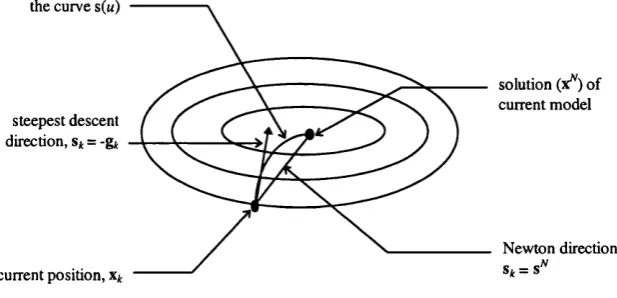
direction; as Uk tends to infinity, Sjt tends to the steepest descent direction - see Figure 3. Strategies for initialising and regulating u are considered in section 3.3.
An important feature of the substitution in Eq. 3.15 is that, if Uk is ‘sufficiently’ large,
will be strictly diagonally dominant - that is, for all i (i = 1,...,»),
Eq. 3.16 ÏÎ,, - ]^|H^.|>0.
j=hj*i
It follows, from the Gerschgorin circle theorem, that such an H is positive definite [Dennis & Schnabel, 1983, 60]. Parameter u can therefore be viewed as providing a mechanism for regulating the positive definiteness of the model Hessian.
Neither line searches nor model-trust region methods are clearly superior. With line
searches, the optimal accuracy with which % approximates the minimum along s* is method- and problem-dependent. With model-trust region methods, the chosen scheme for
initialising and regulating a (or u) can have a significant impact on training performance.
Figure 3 - Parameter u and the model-trust region search direction Note: curve s(m) plots the points = x* + s* for 0 < « <
the curve s(m)
solution (x^) of current model
steepest descent direction, s* = -g*
Newton direction,
St=
current position, x*
3.1.4 Special m ethods for nonlinear least squares
When using the ‘traditional’ sum-of-squares error function
Eq. 3.17
p=\ j= i
(cf. Eq. 2.3), the MLP training task is equivalent to a special category of problem known as nonlinear least squares. Such problems occur when fitting model functions to
experimental data; typically the number of data values m (equivalent to PN^ for an MLP) is greater than the number of free parameters n (equivalent to the number of weights), i.e. the corresponding system of equations is over-determined.
The gradient and Hessian of Eq. 3.17 have a special structure with respect to the residual
vector r and m x n Jacobian matrix J:
Eq. 3.18
In terms of r and J at iteration k.
Eq. 3.20 - 2
Eq. 3.21 gt —
Eq. 3.22 +Sj^
f=]
where is the matrix of second derivatives such that r is the Hessian of r.
Eq. 3.22 is unsuitable as the basis of a general nonlinear least-squares algorithm because the second-order term S is typically unavailable. One option is to ignore S altogether on the assumption that the first-order term of Eq. 3.22 dominates the second-order term near the solution - a reasonable assumption so long as the residuals at the solution are small or zero [Dennis & Schnabel, 1983, 222]. Nonlinear least-squares algorithms which
approximate G according to
Eq.3.23
are considered in section 3.6. A second alternative to Eq. 3.22 is to approximate S by a secant approximation A, i.e.
E q .3.24 G^ = J^Jj^-l-A^ .
Methods derived from Eq. 3.24, which are superior to those derived from Eq. 3.23 for large-residual problems, are considered in [Fletcher, 1980] and [Dennis & Schnabel,
1983, 228-233].
The significance of Eq. 3.23 and Eq. 3.24 is that, given only r* and J*, it is possible to approximate the Hessian matrix G^ immediately at each iteration, whereas with general unconstrained minimisation strategies (such as the quasi-Newton methods of section 3.4)
it may take n iterations to calculate a satisfactory approximation of the {n x n) Hessian.
3.1.5 Scaling and preconditioning
Although none of the classical algorithms considered in the remainder of this chapter are as sensitive to 'sub-optimal' scaling as the steepest descent algorithm (see section 3.1.1), all are prone to numerical problems - ranging from a general degradation in performance and loss of stability to premature termination of the multivariate algorithm - if the scale of either the independent variables x or the function/is sufficiently poor^. Scaling schemes aim to prevent these problems from arising by improving the scale of x (so that the independent variables are of a similar order of magnitude in the 'region of interest') and/or the scale o f/(so that the norm of the model Hessian is of a similar order of magnitude to that of the Hessian itself). A convenient way of approaching the issue of scaling is in term of the condition of the Hessian matrix; a scheme that ensures a problem is 'well-scaled' by minimising the condition number (see Eq. 3.5) of the Hessian - so that similar changes in X lead to similar changes i n /- is known as a preconditioning scheme.
Most scaling schemes modify the scale of x according to the linear transformation
Eq. 3.25 X = Lx ,
where matrix L is fixed and non-singular. The optimal L, which transforms the model Hessian at x* to the identity matrix (assuming G(x*) is positive definite), is
Eq. 3.26 L = G(x.)"''^ ,
where L is a n x n matrix. Assuming G(x*) is not known, the L in Eq. 3.26 can be
approximated using G(xo) (or, if second derivatives are unavailable, a finite-difference approximation of G(xo)). However, unless G is positive definite and remains relatively constant in the region of interest - properties which cannot be guaranteed in general - there is a risk that such a scaling will actually degrade the performance of the
multivariate algorithm. Although it is possible to overcome this problem by recalculating
L periodically {dynam ic scalingor adaptive preconditioning),the high cost of evaluating
G(x) or computing its approximation means that this approach cannot be recommended in a neural network context. Moreover, for methods which have, as one of their main
competitive advantages, 0(n) storage requirements (such as the conjugate gradient methods of section 3.5 and memoryless quasi-Newton method of section 3.4.3), the O(n^) storage cost for matrix L is a significant disadvantage.
The most widely-used scaling schemes for multivariate optimisation represent L in Eq. 3.25 by a diagonal matrix (D). Given a suitable estimate of the condition number of the Hessian (calculated, for example, by the Power method [Mpller, 1993d], or from the Cholesky factors of the Hessian matrix* [Gill, Murray & Wright, 1981, 320-322]), D can be used as a simple preconditioning matrix. Mpller [1993d] has devised an efficient adaptive preconditioning scheme for D, based on an extension to the Power method, which significantly increases MLP training speed with the steepest descent algorithm under most circumstances. However, M0ller reports only a modest improvement for conjugate gradient methods, and concedes that convergence may actually be degraded in some situations (for example, when the Hessian is indefinite).
A simpler alternative is to initialise D according to a set of n user-defined scale factors, representing the approximate ranges of the elements of x. Although this depends on the availability of useful prior knowledge about the problem structure, which cannot be guaranteed for minimisation tasks in general, Rigler et al. [1991] suggest a natural set of scale factors for MLP training derived from the gradient calculation by Eq. 2.1 and Eq. 2.7. When node output y is in the interval [0, 1] (as is the case with the standard sigmoid squashing function of Eq. 2.2), the derivative y' = y*(l - y) (see Eq. 2.8) is constrained so
that 0 < y*(l -y)< 1/4. Given that the factor y*(l - y) is used in the derivative calculation at the preceding layer by Eq. 2.7, Rigler et al. propose that the compensatory factors 6 , 36, 216,... are applied as a multiplier of each partial derivative calculated at layers L-1, L-2, L-3,.... Such a scheme can be modified to take account of the scale of function/. For example Dennis and Schnabel [1983, 209] recommend that the model Hessian is
initialised according to:
Eq. 3.27 Ho = max{]f(xo)|,t}.D^ ,
where r is a user-supplied estimate of the ‘typical’ size of/. (In the absence of any useful information, t is initialised to 1.0 .)
The impact of different scaling schemes on the first- and second-order MLP training algorithms implemented for this thesis is the subject of on-going research. Preliminary experiments suggest that the scale factors proposed by Rigler et al. significantly improve the training speed of first-order algorithms, but not second-order algorithms (although the improvement for first-order methods was not sufficient to bring them up to the speed of any second-order method).
3.2 Line Minimisation
For classical methods with line searches, the task of locating the minimum along search direction Sk (line minimisation) is equivalent to finding the minimum of a function with a single variable (univariate minimisation). For clarity, all the line-minimisation strategies considered here are presented in terms of an arbitrary smooth univariate function/with scalar minimum x*. (Since line minimisation is an iterative process, the suffix m will be used for line-search iterations to prevent confusion with the ^-iterations of the
multivariate algorithm.)
3.2.1 L ine m inim isation strategies
There are two broad strategies commonly used to locate minimum x* of univariate function/: function comparison and function approximation (polynomial interpolation).
Given two initial values of x {Xa and x ^ which hxdick&i x*, function comparison methods iteratively reduce the interval in which x* lies - the interval o f uncertainty - by a fixed ratio. Linear convergence is guaranteed for unimodal functions. (Function/[%) is
the interval at m. In terms of the maximum reduction of the interval for a given number of function definitions, golden section search is almost as efficient as the ‘optimal’ strategy, Fibonacci search. (The latter is considered impractical as it requires the storage or generation of p Fibonacci numbers for p function evaluations, where p is generally not known in advance.)
Function comparison methods are reliable, but make no attempt to exploit the smoothness of function/. The second strategy, polynomial interpolation, approximates/by a simple
function / and uses / to estimate the minimum of/. Typically / is a parabolic
(quadratic) or cubic polynomial. The former requires three pieces of data about/
(typically f(x«), f(xt) and f(Xc)) and the latter four (typically f(x^), g(x^), f{Xb) and g(x^)).
If / is an accurate approximation of/, the theoretical convergence rate is super-linear
(parabolic / ) or quadratic (cubic / ). If, on the other hand, / inaccurately approximates
/, polynomial interpolation is likely to be slow and unreliable; lower-order polynomials may actually prove more accurate than higher-order polynomials in regions where/is comparatively non-smooth^.
3.2.2 Safeguarded polynom ial interpolation
In practice, it is possible to combine the strengths of both the above strategies in a single line-search algorithm with a convergence rate that approaches that of polynomial interpolation under favourable conditions, but remains close to the guaranteed rate of unmodified interval-reduction in the worst case. Such algorithms are termed safeguarded polynomial interpolation algorithms.
Designing such an algorithm is a non-trivial task, requiring efficient and robust mechanisms for detecting how ‘co-operative’ / is and for switching strategies when
appropriate. The method adopted here - Brent’s method [Brent, 1973] - is widely-used and well-regarded [Fletcher, 1980, 29] [Press etal., 1988]. Brent’s method can be implemented with either parabolic or cubic interpolation. Although the latter is likely to
take fewer m-iterations on average, it requires the calculation of derivatives (thereby approximately doubling the computational cost at each m-iteration for an MLP).
3.2.3 Inaccurate line searches
When a line search is used as part of a multivariate minimisation strategy, a key issue is
the accuracy with which a* is chosen to approximate the minimum along s*. The trade-off
between the effort expended to determine an a* of a given accuracy and the corresponding benefit (in terms of the overall reduction in E) to the multivariate algorithm is problem- and algorithm-dependent. Given a sufficiently robust multivariate algorithm, current opinion clearly favours inaccurate line searches on grounds of efficiency.
A practical and popular termination criterion for controlling the accuracy of % is
Eq. 3.28 |g[+,s^|<-^g[s^ ,
where gjt+i is the gradient vector at and q a scalar in the range 0 < g < 1. If <7 is small, an accurate line minimisation is performed, with ^ = 0 giving an ‘exact’ line search. (For exact line searches, the limiting factor is the floating-point precision available; owing to rounding error, it is a waste of effort to evaluate f(x„) if point Xm is closer than the square-root of the machine accuracy to a previously evaluated point [Press etal., 1988, 300].)
To guarantee global convergence it is important that % produces a ‘sufficient’ reduction in E. Since Eq. 3.28 takes no account of the actual reduction in E, it is usual to
supplement it with the condition
E q .3.29 E(x^)-E(xjt-Fa^Sjt)>-Majtg[s^ ,
where u is in the range 0 < w < 0.5. Setting q > u guarantees that Eq. 3.28 and Eq. 3.29 can be satisfied simultaneously.
since s f will satisfy both conditions simultaneously when Xk is close to x* (assuming G is
positive definite), Eq. 3.28 and Eq. 3.29 are compatible with fast rates of local convergence.
To test condition Eq. 3.28 at each m-iteration requires first-derivatives; Eq. 3.28 is, therefore, inappropriate for line minimisation without derivatives. An alternative
condition, proposed in [Gill, Murray & Wright, 1981, 102], replaces the left-hand side of Eq. 3.28 by a finite-difference approximation, i.e.
Eq. 3.30 | E ( x . + a A ) - E ( x . + . J ^ ,
where v is a scalar satisfying 0 < v < a*. For the non-derivative line searches used in this research, Eq. 3.30 was adopted with v=0, so that no additional function evaluations were required to test this condition. Alternatively, Eq. 3.28 can be ignored altogether [Mpller,
1993a], or replaced by a heuristic mechanism for controlling line-search accuracy - for example, Kinsella [1992] places an upper limit on the number of m-iterations performed at a each A:-iteration. However, neither of these alternatives have the theoretical
justifications of Eq. 3.30.
3.2.4 B acktracking line search
Recent results (for conjugate gradient algorithms) published by Mpller [1993a] suggest that inaccurate safeguarded polynomial interpolation - entailing a minimum of three function evaluations per epoch - may be less efficient than the model-trust region approach. However, there is a class of line-search algorithm (not considered by Mpller) which requires only a single function evaluation per epoch in the best case - backtracking line searches.
If the error at Xjt+i = x* + St is unacceptable, backtracking algorithms iteratively
‘backtrack’ (i.e. reduces %) until an acceptable E is found. The algorithm developed here,
based on the backtracking algorithms in [Dennis & Schnabel, 1983], uses parabolic interpolation for the first step and cubic interpolation thereafter. (The latter is performed without expensive derivative calculations by storing f(x^), g(x^) and the two most recent
test values for f(x^ + Pt)-) Parameter u in Eq. 3.29 is set to a small value (10"^) so
that a small reduction in E is sufficient for the acceptance of a given %
Dennis and Schnabel present two versions of their backtracking algorithm; one version - the ‘modified’ version - implements Eq. 3.28 and requires derivative calculations, the other does not. The authors give theoretical and practical reasons for implementing Eq. 3.28 as well as Eq. 3.29 with algorithms that use quasi-Newton approximations to the Hessian matrix. With the architectures, training problems and multivariate algorithms considered in this research, the Dennis-Schnabel unmodified backtracking algorithm displayed worse average convergence characteristics than the modified algorithm. The non-derivative backtracking algorithm developed here, which implements Eq. 3.30 rather than Eq. 3.28 (with a corresponding saving in derivative calculations), retained the improved performance of the modified Dennis-Schnabel algorithm.
3.2.5 H ybrid Brent/backtracking line search
In trials conducted for this research it was observed that low-accuracy non-derivative Brent’s method frequently made better progress than the backtracking strategy in very flat regions - a common feature of MLP error surfaces (see section 2.2.1). In response to this observation, a novel hybrid Brent/backtracking algorithm has been developed. This algorithm uses the efficient backtracking strategy under ‘average’ conditions but switches to Brent’s method under unfavourable conditions, i.e. whenever the number of
3.2.6 Line search im plem entation
Multivariate vj. univariate implementation. Line-search algorithms can be coded either
using vector-valued points or (as here) scalar points. The second alternative requires some mechanism for evaluating the multi-dimensional function F in a single dimension; the simple device adopted here (described in [Press et al., 1988, 317]) is to provide an
‘artificial’ uni-dimensional function f(a) which evaluates F at + ocxjt.
Handling non-descent directions. A prerequisite for all the line searches considered
above is that Sk satisfies Eq. 3.9 (i.e. Sk is a descent direction). Sk is guaranteed to satisfy Eq. 3.9 with the SD algorithm, so long as the gradient is greater than zero. However,
many multivariate algorithms do occasionally generate an s* which is not a descent direction (for the various reasons considered in section 3.1). In these circumstances, probably the only solution (in general) is to restart the multivariate algorithm at the current position, with s reset to the steepest descent direction. An unfortunate by-product of resetting the algorithm is that any useful derivative information from previous
iterations will be automatically discarded.
3.3 Model-Trust Region Strategies
The model-trust region approach has become an increasingly popular alternative to the traditional line-search approach. For all the strategies considered here, it is assumed that
the step length (radius) a* is controlled indirectly by parameter u via the substitution in Eq. 3.15. There is no ‘natural’ choice for mq; recommended settings range between 0.001
[Press et al., 1988] and < 10"°^ [M0ller, 1993a].
3.3.1 A sim ple m odel-trust region algorithm
The simplest model-trust region strategy is given by the following pseudo-algorithm
(based on the Levenberg-Marquardt algorithms in [Press et al., 1988] and [Nash, 1990]):
1. Set uq > 0;
2.2. IF f(xt 4- St) < f(xt),
2 .2 .1. set Xjt+i = Xjfe + Sjt;
2 .2 .2 . divide by a reduction constant",
ELSE
2.2.3. set Xk+\ = Xk,
2.2.4. multiply Uk by a growth constant.
For this research, the reduction constant was set to 2 or 4 and the growth constant to 4 or 10. This strategy has proved satisfactory when used with the Levenberg-Marquardt method of section 3.6, but is prone to inefficient, oscillatory behaviour in regions where the appropriate value of u remains relatively constant for a number of iterations. (This behaviour is particularly apparent if the reduction and growth constants are set to the same value, as advocated by [Press et al., 1988].)
3.3.2 F letcher’s m ethod
A better strategy - sometimes called Fletcher's method [Wolfe, 1978] - is to chose a Uk that ensures ‘sufficient’ agreement is maintained between the actual and predicted
quadratic error change at each iteration (AEk and AQk respectively). This is conveniently measured in terms of the ratio r, given by
Eq. 3.31 = *
AG,
The predicted error change AQk can be calculated as follows:
Eq. 3.32 AG, = E , - G(s^ )
0 (sj) = |s [ G ^ S j + g [s j
This leads to the following pseudo-algorithm (based on the Levenberg-Marquardt algorithm in [Fletcher, 1980]):
1. Set « 0 > 0;
2. While termination criteria are not satisfied, 2 .1. calculate s^;
ELSE IF Tk is greater than upper ratio limit w, 2.3.2, divide Uk by a reduction constant', ELSE
2.3.3, set Mjt+i = Mjk; 2,4, IF r, < 0
2.4.1, set Xjfc+] = Xjt; ELSE
2.4.2, set Xjt+i =Xk + s^.
The lower and upper ratio limits v and w are typically chosen so that 0 < v < w < 1, This algorithm is relatively insensitive to changes in the various constants; those used in this research are the same (arbitrary) constants advocated in [Fletcher, 1980, 96]: v=0,25 and w=0,75, (Settings for the growth and reduction constants were the same as for the simple strategy of section 3,3,1,)
When G is not available (as, for example, with conjugate gradient methods), G^St (in Eq, 3,32) can be approximated by a one-sided finite-difference approximation or calculated exactly with P forward and backward passes using an algorithm described in [Mpller,
1993c], Both schemes have 0(PN) time and storage costs; on average, the former yields a faster convergence rate than the latter (which is prone to numerical instability) [Mpller, 1993e, 39],
3.3.3 M odern m odel-trust region algorithm s
More recent model-trust region strategies choose Uk so that Eq, 3,14 is satisfied explicitly at each iteration, i,e, a Uk that satisfies
Eq. 3.33 ||s^|| = a^
whenever the length of is greater than % [More, 1983], Two strategies for iteratively
approximating the Uk that satisfies Eq, 3,33 - the locally constrained optimal ('hook') step and the double dogleg step - are presented in [Dennis & Schnabel, 1983, 134],
3.4 Quasi-Newton Methods
Quasi-Newton (QN) methods^^ differ from Newton’s method in that an approximation of
the Hessian matrix (or its inverse) is built up iteratively, rather than calculated afresh at each epoch. Since QN algorithms do not require analytic second derivatives, they are more suitable for MLP implementation than straight Newton-type methods.
3.4.1 T he H essian update form ula
In generating the Hessian approximation H^+i from Ht using the derivative information collected during iteration k, all QN methods satisfy the so-called quasi-Newton
condition^ ’
Eq. 3.34 H^+iP^ = ,
where yt and pt are respectively the gradient change and the change in position x during iteration Ac, i.e.
Eq. 3.35 y t = Agj = g.^., - gj
Pt =AXj = X j ^ , - X j .
Where methods differ is in the choice of updating formula that satisfies Eq. 3.34. Ho is typically set to the identity matrix (I) as a ‘neutral’ first approximation, making the first iteration equivalent to steepest descent.
QN methods are categorised in terms of the simple equation
Eq. 3.36 H^^i = H^ ,
There is some confusion in the numerical analysis literature about the use of the terms 'quasi-Newton methods', 'variable metric methods', and 'secant methods'; some authors maintain a distinction between these terms (see, for example, [Dennis & Schnabel, 1983]), others do not. In this research, the term 'quasi-Newton methods' is used throughout.
where C* is a correction or update matrix. The best-known methods use a rank-two matrix for C*: the Davidon-Fletcher-Powell (DFP) update (most concisely written in terms of the inverse model Hessian, H )
Eq. 3.37 = H^' + ,
p ly . y lH j'y .
and the Broyden-Fletcher-Goldfarb-Shanno (BFGS) update (the complement of the DFP
update) given by
Eq. 3.38 =H *
y . P . P . H jP j
Under various fairly stringent conditions (including the strict convexity off) both DFP and BFGS methods are globally convergent with a super-linear rate of local convergence. However, there is overwhelming theoretical and experimental evidence that the BFGS update is superior to the DFP update (and probably all other updates) [Dennis & Schnabel, 1983] [Dixon, 1972] [Fletcher, 1980]. (The DFP update has, for instance, the reputation of being highly sensitive to the choice of line-search accuracy.)
3.4.2 R epresenting the H essian approxim ation m atrix
If the Hessian approximation H is represented directly, QN methods - like Newton’s method - require the solution of Eq. 3.8 at the cost of O(n^) multiplications per iteration. By storing an approximation of the inverse Hessian G rather than G itself, the cost falls to O(n^) multiplications. In terms of the inverse Hessian, the BFGS update Eq. 3.38 becomes
Eq. 3.39 H"!, = H - ' +
p l y . p . y . p . y .