University of Pennsylvania University of Pennsylvania
ScholarlyCommons
ScholarlyCommons
Publicly Accessible Penn Dissertations
2019
Reinforcement Learning With High-Level Task Specifications
Reinforcement Learning With High-Level Task Specifications
Min Wen
University of Pennsylvania, [email protected]
Follow this and additional works at: https://repository.upenn.edu/edissertations
Part of the Artificial Intelligence and Robotics Commons
Recommended Citation Recommended Citation
Wen, Min, "Reinforcement Learning With High-Level Task Specifications" (2019). Publicly Accessible Penn Dissertations. 3509.
Reinforcement Learning With High-Level Task Specifications
Reinforcement Learning With High-Level Task Specifications
Abstract Abstract
Reinforcement learning (RL) has been widely used, for example, in robotics, recommendation systems, and financial services. Existing RL algorithms typically optimize reward-based surrogates rather than the task performance itself. Therefore, they suffer from several shortcomings in providing guarantees for the task performance of the learned policies: An optimal policy for a surrogate objective may not have optimal task performance. A reward function that helps achieve satisfactory task performance in one environment may not transfer well to another environment. RL algorithms tackle nonlinear and nonconvex optimization problems and may, in general, not able to find globally optimal policies. The goal of this dissertation is to develop RL algorithms that explicitly account for formal high-level task specifications and equip the learned policies with provable guarantees for the satisfaction of these specifications. The resulting RL and inverse RL algorithms utilize multiple representations of task specifications, including conventional reward functions, expert demonstrations, temporal logic formulas, trajectory-based
constraint functions as well as their combinations. These algorithms offer several promising capabilities. First, they automatically generate a memory transition system, which is critical for tasks that cannot be implemented by memoryless policies. Second, the formal specifications can act as reliable performance criteria for the learned policies despite the quality of the designed reward functions and variations in the underlying environments. Third, the algorithms enable online RL that never violates critical task and safety requirements, even during exploration.
Degree Type Degree Type
Dissertation
Degree Name Degree Name
Doctor of Philosophy (PhD)
Graduate Group Graduate Group
Electrical & Systems Engineering
First Advisor First Advisor
Ufuk Topcu
Second Advisor Second Advisor
George J. Pappas
Keywords Keywords
Game theory, Inverse reinforcement learning, Learning-based control, Learning from demonstration, Reinforcement learning, Temporal logic specifications
Subject Categories Subject Categories
REINFORCEMENT LEARNING WITH HIGH-LEVEL TASK SPECIFICATIONS
Min Wen
A DISSERTATION
in
Electrical and Systems Engineering
Presented to the Faculties of the University of Pennsylvania
in
Partial Fulfillment of the Requirements for the
Degree of Doctor of Philosophy
2019
Supervisor of Dissertation
Ufuk Topcu, Assistant Professor of Aerospace Engineering and Engineering Mechanics, Univ. of Texas at Austin
Graduate Group Chairperson
Victor Preciado, Associate Professor of Electrical and Systems Engineering
Dissertation Committee
George J. Pappas, Joseph Moore Professor and Chair of Electrical and Systems Engineering
Manfred Morari, Distinguished Faculty Fellow of Electrical and Systems Engineering
REINFORCEMENT LEARNING WITH HIGH-LEVEL TASK SPECIFICATIONS
c
COPYRIGHT
2019
Min Wen
This work is licensed under the
Creative Commons Attribution
NonCommercial-ShareAlike 3.0
License
To view a copy of this license, visit
ACKNOWLEDGEMENT
First and foremost, I would like to express my deepest gratitude to my advisor, Ufuk Topcu. Without
his continuous encouragement, trust, and patience throughout my studies, it would be impossible
for me to explore the diverse research topics in my thesis and find my own research story there. His
enthusiasm for research and working and his positive attitude in face of all difficulties have shaped
my understanding of being a researcher and a reliable person. It is my fortune to have him as my
advisor and friend.
I would like to thank my thesis committee members, Professor George Pappas, Manfred Morari, and
Michael Littman, for generously sharing their vision and wisdom with me. I also learned a lot by
attending George’s group meetings in the past few years.
I thank my friends for our memorable times together: Ximing Chen, Bhoram Lee, Jinwook Huh,
Sangdon Park, Meng Xu, Siyao Hu, Clark Zhang, Ivan Papusha, Shaoru Chen, Lingjun Chen, and
Konstantinos Gatsis. I am also very lucky to have two of my high-school deskmates, Ning Wang and
Meng Ye, to pursue our PhDs together in Philadelphia.
Finally, I would like to thank my parents, Dan Liu and Kewu Wen. Thank you for being my parents,
raising me with all your love, and always supporting me to pursue my dreams. I also thank my
grandfather, Taiji Liu, for sharing his own experience with me when I get puzzled and upset. I will
always benefit from his positive attitude towards life. I thank my husband, Jihua Huang, for his love,
ABSTRACT
REINFORCEMENT LEARNING WITH HIGH-LEVEL TASK SPECIFICATIONS
Min Wen
Ufuk Topcu
Reinforcement learning (RL) has been widely used, for example, in robotics, recommendation
systems, and financial services. Existing RL algorithms typically optimize reward-based surrogates
rather than the task performance itself. Therefore, they suffer from several shortcomings in providing
guarantees for the task performance of the learned policies: An optimal policy for a surrogate
objective may not have optimal task performance. A reward function that helps achieve satisfactory
task performance in one environment may not transfer well to another environment. RL algorithms
tackle nonlinear and nonconvex optimization problems and may, in general, not able to find globally
optimal policies. The goal of this dissertation is to develop RL algorithms that explicitly account
for formal high-level task specifications and equip the learned policies with provable guarantees for
the satisfaction of these specifications. The resulting RL and inverse RL algorithms utilize multiple
representations of task specifications, including conventional reward functions, expert demonstrations,
temporal logic formulas, trajectory-based constraint functions as well as their combinations. These
algorithms offer several promising capabilities. First, they automatically generate a memory transition
system, which is critical for tasks that cannot be implemented by memoryless policies. Second, the
formal specifications can act as reliable performance criteria for the learned policies despite the
quality of the designed reward functions and variations in the underlying environments. Third, the
algorithms enable online RL that never violates critical task and safety requirements, even during
TABLE OF CONTENTS
ACKNOWLEDGEMENT iv
ABSTRACT v
LIST OF TABLES viii
LIST OF ILLUSTRATIONS xi
1 Introduction 1
1.1 Challenges in Representing Task Requirements as Reward Functions . . . 1
1.2 Outline and Contributions . . . 4
1.3 Related Work . . . 7
2 Learning from Demonstrations with High-Level Side Information 17 2.1 Introduction . . . 17
2.2 Preliminaries . . . 18
2.3 Maximum-Likelihood Inverse Reinforcement Learning (MLIRL) . . . 21
2.4 MLIRL with High-Level Side Information . . . 22
2.5 Experimental Results . . . 26
3 Task-Oriented Deep Inverse Reinforcement Learning 32 3.1 Introduction . . . 32
3.2 Preliminaries . . . 34
3.3 Task-Oriented Deep Inverse Reinforcement Learning . . . 37
3.4 Related Work . . . 39
3.5 Experimental Results . . . 41
4.1 Introduction . . . 46
4.2 Related Work . . . 48
4.3 Preliminaries . . . 49
4.4 Constrained Cross-Entropy Framework . . . 53
4.5 Experimental Results . . . 74
5 Correct-By-Synthesis Reinforcement Learning with Temporal Logic Constraints 82 5.1 Introduction . . . 82
5.2 Preliminaries . . . 84
5.3 Problem Formulation . . . 88
5.4 Permissive Strategies, Learning and the Main Algorithm . . . 90
5.5 Experimental Results . . . 96
6 Probably Approximately Correct Learning in Stochastic Games with Temporal Logic Specifications 101 6.1 Introduction . . . 101
6.2 Related Work . . . 103
6.3 Preliminaries . . . 104
6.4 Problem Formulation . . . 109
6.5 Main Approach . . . 110
6.6 Proof of Theorem 6 . . . 122
6.7 Experimental Results . . . 137
7 Conclusion 142 7.1 Future Research Directions . . . 144
LIST OF TABLES
TABLE 1 : Design of features in Case 2 and Case 3. . . 27
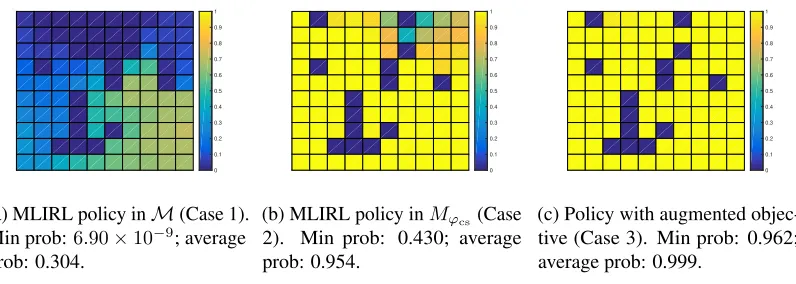
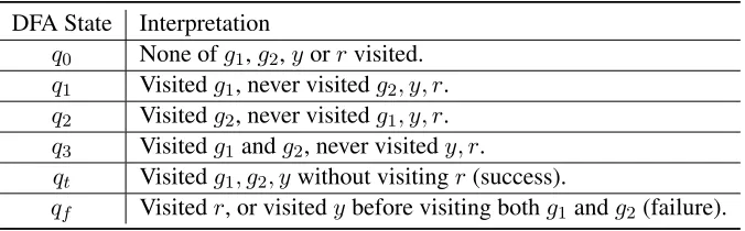
TABLE 2 : Interpretation of DFA states. . . 29
TABLE 3 : DFA states . . . 42
TABLE 4 : Ji(τ),Zi(τ)and constraint upper bounddifori= 1,2,3,4,τ ∈(S×A)N. 79
TABLE 5 : Results for example 1. . . 97
LIST OF ILLUSTRATIONS
FIGURE 1 : Illustration of the grid world example. Left: grid world map and
demon-stration trajectories. Right: an equivalent DFA forϕcs. . . 26
FIGURE 2 : Probability of satisfyingϕcswhen following the corresponding policy
from each initial state. . . 28
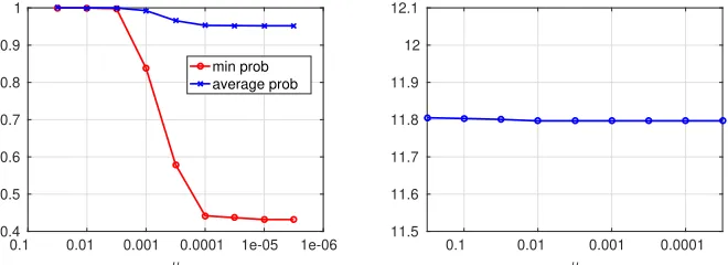
FIGURE 3 : Probability of satisfyingϕcs (left) and negative log-likelihood of the
state-action pairs in demonstration (right), as function ofµ. . . 30
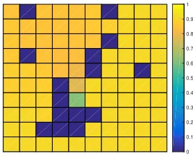
FIGURE 4 : Probability of satisfyingϕcs for policies learned without the obstacle
avoidance requirement. . . 31
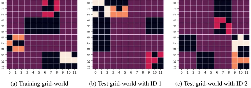
FIGURE 5 : Training and test grid-worlds. Indexing convention: (vertical axis index,
horizontal axis index). In (a)O1 = (1,7),O2 = (7,1),O3 = (10,10)
andOB = {(4,4),(4,5),(4,6),(4,7),(10,7)}. All other cells
corre-spond to distractor objects. . . 42
FIGURE 6 : Training and testing performance of TODIRL and the baselines with 100
demonstrations. . . 44
FIGURE 7 : Testing performance with 100 demonstrations for different design choices. 45
FIGURE 8 : Comparison of the globally optimal policyπ∗and the 50 learned policies
for different policy network structures. Each row corresponds to a policy
network structure. From left to right, the first three columns represent
the trajectories of the two statesxt(1),xt(2)and the inpututover time
t. The solid line in each figure is forπ∗and the dashed lines are for the
learned policies. In the fourth column, we show the gap between their
G-values andG(π∗)in ascending order. In the last column, we show the
FIGURE 9 : (9a) Map of the 2D navigation example. There are one obstacle region
(grey rectangle), one goal region (blue rectangle) and 10 randomly selected
initial states (red circles pointing to the forward direction). Dotted lines
are added to showxand yaxes. (9b) Illustration of the local features
in the robot’s local coordinate at one of the initial states, withns = 5.
Obstacle nodes, goal nodes and free nodes are labeled by black crosses,
yellow plus signs and green triangles respectively. The goal direction
(black arrow) is also included in local features. . . 78
FIGURE 10 : Learning curves of CCE, CPO and TRPO with different objectivesGJi
and constraintsHZi. The horizontal axes show the total number of sample
trajectories for CCE and the total number of equivalent sample trajectories
for TRPO and CPO. The vertical axes show the sample mean of the
objective and constraint values of the learned policy (for TRPO and CPO)
or the learned policy distribution (for CCE). The shade shows 1 standard
deviation. The region below the dashed line in the second row is feasible.
Each experiment is repeated for 5 times. . . 80
FIGURE 11 : Average performance of CCE, CPO and TRPO for Experiment 4 with
initial feasible policy. . . 81
FIGURE 12 : A gameG0without finite-memory optimal strategy. . . 89
FIGURE 13 : Results for Example 1 forN = 4: (Left)J¯RGˆ(ˆµ,s)ˆ for allsˆ∈Ssˆ and the
learned greedy strategyµˆ; (right) the logarithm of the maximal change in
V in every104iterations. . . 98
FIGURE 14 : Result for Example 2 whenN = 4: J¯Gˆ1
R(ˆµ,s)ˆ for allsˆ∈Sˆsand a learned
greedy strategyµˆ. . . 99
FIGURE 15 : DBA constructed for some example specifications. Accepting states for
FIGURE 16 : Illustration of the construction ofGˆ =HatGame(G, Q∗, ε0, pε0). Each
arrow represents an available action from the starting state. The red
arrows correspond toε0-optimal actions inA∗ε0(s). For each system state
s ∈ Ss in G, there are three states in Gˆ: a copy of the state s with
only one available actionaˆ, and two virtual statess1 ands2 such that
AGˆ(s1) =AG(s)andAGˆ(s2) =A∗ε0(s). . . 118
FIGURE 17 : (17a) A DBA constructed for the example. p1stands for the lower left
block, andp2stands for the upper right block. (17b) The optimal strategy
for the system with only the discounted reward. The pink and blue squares
represent the dangerous areas when the light is on and off. The triangles
show the optimal transition directions from each block (pink ones for light
on, blue ones for light off). . . 137
FIGURE 18 : Comparison of the value function of the initial almost-sure winning
strat-egy, the learned strategy and an optimal strategy (which may not be
almost-sure winning) for all system states. The red crosses mark all the
strongly connected components in which there is at least one state whose
value is learned to beε-optimal. . . 139
FIGURE 19 : Illustration of the initial almost-sure winning strategyσs (the middle
column) and the learnedε-optimal almost-sure winning system strategy
σs,ε (the right column). From top to bottom, the four figures in each
column show the system strategy with DBA stateq1toq4. In each figure,
the pink and blue triangles point to the transition directions at each block
when the light is on and off respectively. In the right column, big triangles
represent actions with probability(1−pε1), and small triangles represent
actions with probabilitypε1. Triangles with yellow background areε
Chapter 1: Introduction
Reinforcement learning (RL) techniques have been used to solve a wide range of real-world tasks
such as robotics [55, 68, 83, 85, 91, 196], recommendation systems [109, 172, 199] and financial
services [45, 118, 128]. Given a reward function and some mechanism for a learning agent to interact
with its environment, the goal of RL is to learn anoptimalpolicy that maximizes the expected reward.
To solve a robotic task using RL, one first needs to specify a reward function to encode the task
objective, which implicitly introduces the following assumption:
The more expectedrewarda policy gets, the bettertask performanceit has.
In other words, the assumption states that the expected reward is interpreted as a performance
criterion for the given task. This assumption holds trivially for score-optimizing applications such as
board games [100, 161, 162] and video games [122, 132], where a lot of impressive RL applications
emerge these days. However, this assumption is rarely valid for most real-world tasks, where reward
functions are not part of the original task specification and need to be designed. In general, reward
design is non-trivial and mostly still an open problem [9, 69, 163, 200]. In many cases, reward
design proceeds by trial and error with intense human supervision, yet the learned policies still lack
guarantees for task performance. In Section 1.1, we show several reasons why a reward function by
itself is not an ideal way to represent task requirements in general.
1.1. Challenges in Representing Task Requirements as Reward Functions
Conceptually, there is a non-negligible gap between the objective of reward design and the
require-ment of reward utilization. For reward design, the goal is usually to find a candidate reward function
such that there existsan optimal policy that implements the given task successfully in training
environments, as in the cases of ad-hoc reward design and inverse reinforcement learning [1]. For
reward utilization, it is required thatalloptimal policies with the specified reward function can
implement the task successfully in (possibly different)testingenvironments, as any optimal policy
i.e., a reward function that assigns zero rewards to all state-action pairs. A policy that implements the
given task successfully is undoubtedly optimal for the all-zero reward function; nevertheless, it is
impractical to learn such a policy using such an uninformative reward.
For some relatively simple tasks, it is possible to bridge this gap usingsparserewards. Consider a
target-reaching task as an example, where the goal is to reach a given target object within ten time
steps. Then a reward function that satisfies the above assumption can be designed as follows: The
reward is one if the hand has just reached the target object and zero otherwise. With this reward
function, any optimal policy that maximizes the expected total reward maximizes the probability
to reach the target object within ten steps. However, the sparsity of non-zero reward signals makes
exploration very inefficient and thus is undesired for most RL algorithms.
For more complicated tasks, reward functions need to encode multiple (possibly conflicting)
long-term objectives, where each objective corresponds to some behavior to be encouraged or prohibited.
The objectives can still be quantified separately as reward basis functions, but their weights that
signify the importance of each basis function to task performance are not apparent. Even for a
specific weight vector, it is not clear how to predict the task performance of the corresponding
optimal policies without actually solving the RL problem. Moreover, the trade-off between the basis
functions is also affected by the system dynamics and the underlying environment. Therefore, a
reward function that leads to good task performance in one environment may not guarantee similar
performance in another environment, which suggests that it may not be enough to represent task
requirements merely as reward functions.
Last but not least, RL techniques may not always converge to a global optimum, especially when
nonlinear parameterization is used, which is almost always the case for problems with continuous
state spaces. Recently, deep RL techniques [108] becomes popular, where the agent’s policy is
parameterized as a neural network. The network weights are computed using backpropagation and
updated using some stochastic gradient descent method. There is no wonder that neither the expected
reward nor the task performance is convex in network weights, and thus gradient-based methods
details of deep RL algorithms such as policy network structure, batch size, learning rate, and even
random seeds can drastically alter the performance of deep RL algorithms [71]. This observation
again indicates that it is impractical to rely on reward design to guarantee the task performance of the
learned policies.
Having discussed the limitations of reward-based task specifications, we also note that reward function
is neither the unique way nor the most common way for humans to describe task requirements. Rather
than optimizing some quantitative evaluative feedback (such as rewards) from each transition, it is
far more natural to learn from high-level task requirements in natural language or to directly imitate
some successful demonstrations of the given task. For example, when people learn to drive, they are
required to learn the road rules to follow some general guidelines and avoid some common mistakes.
In the meantime, they learn about driving customs by both mimicking the other drivers and observing
others’ feedback. Similarly, we can express the rule-based task requirements as temporal-logic-based
specifications or finite-state transition systems, and consider expert demonstrations as a given set of
trajectories.
Instead of relying on reward functions as a unique task description, we propose to incorporate
miscellaneous sources of task information into RL algorithms, with the following objective in mind:
To learn policies that areknownto have reliable task performance.
The exploitation of reward-free task information can help improve output task performance in
multiple ways. For example, constraints help restrict the search space of output policies: Trajectories
generated by a valid output policy should satisfy the given constraints with high probability. Temporal
logic specifications show insights into task structure and facilitate the design of memory states. Expert
demonstrations provide samples of desired behaviors for policy training and the inference of the
expert’s preferences. The works in this dissertation are some exploratory steps towards the ultimate
1.2. Outline and Contributions
The overarching goal of this dissertation is to utilize different sources of available task information
besides reward functions and provide the policies learned by reinforcement learning with task
performance guarantees. The works in this dissertation contain three parts, where each part uses
different formulations and task representations.
1.2.1. Learning from Demonstrations with High-Level Side Information
The first part includes Chapter 2 and Chapter 3, in which we represent the task information in the
following two ways: First, there is a co-safe linear temporal logic specification or an equivalent
deterministic finite automaton [99], which can be used to directly check whether a given trajectory
fails or succeeds in the given task. Additionally, there is a set of demonstrations showing how
an experienced expert implements the given task. The overall problem, formulated as an inverse
reinforcement learning problem, aims at learning a reward function and an output policy at the same
time such that the learned policy satisfies the given temporal logic specification with high probability.
Chapter 2 shows how to extend an existing inverse reinforcement learning algorithm (the example
used in Chapter 2 is the maximum likelihood inverse reinforcement learning algorithm [12]) to
explicitly take advantage of the extra input of task information as a co-safe linear temporal logic
specification. The proposed algorithm incorporates the task information in several steps. First, it
transforms the specification into an equivalent deterministic finite automaton, such that a trajectory
satisfies the specification if and only if it is accepted by the deterministic finite automaton. Then the
algorithm constructs a product automaton by extending the state space of the original environment
with the deterministic finite automaton. Essentially, the deterministic finite automaton acts as a
memory transition system that tracks the current progress of the task, since the policies of the
product automaton depend on both the current state in the environment Markov decision process
and the state in the task deterministic finite automaton. Moreover, there is a one-to-one mapping
between the trajectories of the environment Markov decision process and the trajectories of the
learned policy satisfies the temporal logic specification, can be evaluated in the product automaton
and is independent of the recovered reward function. As the task performance is differentiable,
it can be used to augment the objective function of the underlying inverse reinforcement learning
algorithm. The resulting algorithm parameterizes the reward function as a linear combination of a set
of manually designed reward features in the constructed product automaton.
Chapter 3 extends the above framework to nonlinearly parameterized reward functions such as
reward networks. The proposed algorithm relies on an existing deep maximum-entropy inverse
reinforcement learning algorithm [195]. While the previous work focused on the generalization
performance at states without expert demonstrations in the same environment, this work evaluates the
generalization performance in new testing environments with no expert demonstrations. Compared
with linearly parameterized rewards, reward networks gain the capability to construct reward features
automatically and thus transferable to new environments. After transferring the learned reward
function, the algorithm computes a new policy separately for each testing environment. A comparison
of the generalization performance of the proposed algorithm with that of a memory-based behavioral
cloning algorithm shows that, with the same set of expert demonstrations, policies generated by the
learned reward function have near-perfect task performance in both training and testing environments,
while the policy learned by the memory-based behavioral cloning algorithm deteriorates significantly
in testing environments.
1.2.2. Constrained Reinforcement Learning
The second part corresponds to Chapter 4. In this part, we represent task information as objective
and constraint functions and formulate the problem as a constrained reinforcement learning problem.
The constraint functions act as the role of temporal logic specifications in the first part: a policy
isfeasibleif and only if all constraint functions evaluated with this policy are within the specified
ranges. The objective function encodes preferences over different feasible policies. Both objective
and constraint functions are evaluated over finite-step trajectories and thus can encode even
We treat both objective and constraint functions as black boxes and propose a constrained
cross-entropy-based method. The key idea is to transform the original constrained optimization problem
into an unconstrained one with a surrogate objective. The method explicitly tracks its performance
for constraint satisfaction and thus is well-suited for safety-critical applications. We show that
the asymptotic behavior of the proposed algorithm converges almost-surely to that of an ordinary
differential equation, and also provide sufficient conditions on the differential equation for the
convergence of the proposed algorithm. We illustrate the performance of the proposed algorithm with
two simulation examples. The first one is a constrained linear quadratic regulator problem, in which
the algorithm converges to the global optimum with high probability. The second example is a 2D
navigation problem, for which the proposed algorithm manages to learn feasible policies effectively
without assumptions on the feasibility of initial policies, even with non-Markovian objective functions
and constraint functions.
1.2.3. Reinforcement Learning with Temporal Logic Constraints in Two-Player Games
The third part includes Chapter 5 and 6. In this part, we consider two reinforcement learning
problems in two-player games, where the task requirements are represented by one qualitative
and one quantitative objective. Similar to the first part, we represent the qualitative objective as
a temporal logic specification that is not limited to the co-safe ones. No matter which policy the
other uncontrolled player takes, the learning agent should guarantee to satisfy the given temporal
logic specification even during the learning procedure. The quantitative objective is the worst-case
expected discounted reward, which is unknown a priori and learned by interacting with the other
player. The two objectives are independent of each other such that they may be conflicting, somewhat
similar, or irrelevant at all.
In Chapter 5, we model the interaction between a controlled agent (referred to as thesystemagent)
and an uncontrolled agent (referred to as theenvironmentagent) a deterministic two-player
turn-based zero-sum game. Since the two objectives are independent, we decouple the two objectives
and address them separately. In this work, the algorithm first computes, for the system agent, a
includes multiple (possibly all) policies that guarantee the system to satisfy the given specification,
despite the policy of the potentially adversarial environment agent. The algorithm restricts the system
agent to take the policies included in the permissive strategy and solves an optimal system policy
over the restricted set using any RL algorithms for zero-sum two-player games. For a particular
case where the given temporal logic specification encodes a safety property, this two-step technique
secures both correctness (with the safety property) and optimality (with the a priori unknown reward
function). For other specifications, the learned policy still satisfies the given specification but may be
sub-optimal.
Chapter 6 generalizes the previous problem in two ways. First, the game transitions can be stochastic
instead of deterministic; second, it addresses a broader type of temporal logic specifications without
loss of optimality. In this work, we assume that the given temporal logic specification is representable
as a deterministic B¨uchi automaton, which strictly includes the safety property. The quantitative
objective is to maximize the expected discounted reward over an infinite horizon. We prove that there
always exists amemoryless almost-sure winningstrategy that isε-optimal for any arbitrary positive
ε. Based on the idea of the R-MAX algorithm [28], a probably approximately correct (PAC) learning
algorithm is proposed to learn such a strategy efficiently in an online manner with a priori unknown
reward functions and unknown transition distributions. To the best of our knowledge, this is the first
result on PAC learning in stochastic games with independent quantitative and qualitative objectives.
1.3. Related Work
In this section, we introduce two fields of works, namely learning from demonstrations and
learning-based control with safety requirements, that are closely related to the high-level idea of this thesis.
For each field, we describe the high-level ideas, main existing approaches, and their connections with
high-level task specifications.
1.3.1. Learning from Demonstrations
Chapter 2 and 3 of this thesis is closely related to the topic of learning from demonstrations (LfD) [10],
some unknown expert policy, learn a policy toimitatethe expert demonstrations. The interpretation
of imitation varies among different LfD methods. In general, there are two types of approaches to
LfD problems: behavioral cloning, and inverse reinforcement learning.
Behavioral cloning. Behavioral cloning methods directly formulate the LfD problem as a
super-vised learning problem. In other words, behavioral cloning directly reproduces a mapping from states
to actions or action distributions that will be taken by the expert. Depending on whether actions are
continuous or discrete, behavioral cloning methods can be classified into regression or classification
methods. The strength of behavioral cloning has been demonstrated by various applications that
range from basic navigation tasks such as lane keeping [142] to complicated tasks such as obstacle
avoidance [78, 151] and end-to-end autonomous driving [25, 126].
Behavioral cloning methods suffer from the following two noticeable limitations.
The first limitation is oncompounding errorsorcascading errors[149]: The difference between the
state distributions induced by the expert policy and the learned policy compounds over time. For
behavioral cloning, testing performance is not evaluated over a randomly drawn subset of states from
expert demonstrations (which is a common practice for standard supervised learning problems), but
rather over the distribution of state-action pairs generated by executing the learned policy. As the
action distributions at previous steps affect the state distributions at later steps, the state distribution
induced by a learned policy gradually diverges from that of the expert policy as time goes on. As a
result, the learned policy often guides the agent to reach states that are distinct or far away from the
states in the expert demonstrations. It is not clear to the agent how to behave at these states, or how
to return to states visited in demonstrations.
Another limitation of behavioral cloning is the inability to replan in new environments. For the
policies trained by supervised learning methods, the predicted action distribution at each state is only
decided by the local features of that state and independent of the possible states to be visited later.
As a result, the learned policies ignore the long-term effect of each action and “(behavioral cloning)
Various attempts have been made to overcome the above two limitations. The key idea is to allow the
learning agent to query the expert’s policy at any given state. Based on this idea, Ross and Bagnell
[149] first proposed the SMILe algorithm to stochastically combine the expert policy and the policies
learned in each iteration, and gradually reduce the probability to query the expert over time. Ross et
al. [150] proposed another algorithm called DAgger that augments the demonstration data in each
iteration with the expert’s new demonstrations on all states visited by the learned policy. Laskey et al.
[101] forced the expert to demonstrate how to recover from errors by injecting noise into the expert’s
policy during the demonstrating process.
Inverse reinforcement learning. Inverse reinforcement learning (IRL) [129], also called inverse
optimal control [84], solves the LfD problem in an indirect manner: It assumes that the expert policy
optimizes the expected reward with some unknown reward function, and thus IRL methods aim at
inferring a reward function from the given expert demonstrations. IRL is closely related to (forward)
RL, which solves optimal policies for some given reward function. Many IRL algorithms need to
solve an RL problem after each update of the learned reward function. IRL methods have been used
in many applications such as flying helicopters [2, 3], navigation of mobile robots [96, 187, 195],
goal inference [14], behavior modeling of pedestrians [52] and drivers [98], to name a few.
IRL problems suffer from the problem ofill-posedness: For example, the all-zero reward function
admits any policy as its optimal policy and thus is a sound solution for any expert demonstrations. A
given policy can be optimal simultaneously for many different reward functions, and the optimal
policies for these reward functions are generally not equivalent. Therefore, it is upon each IRL
algorithm to decide how to interpret the expert demonstrations with the expert’s reward function
or with the output policy. These algorithms typically resort to some common heuristics: First, the
expected reward of the expert policy (estimated as the average value over expert demonstration)
matches that of the learned policy [1, 201]. Second, the expected reward of the expert policy is
higher than that of any other policies by a given margin [147]. Third, the output policy maximizes
Challenges of LfD for task implementation. Remember that our goal is to learn how to
imple-ment high-level tasks from expert demonstrations. However, most existing LfD algorithms merely
rely on statistical analyses of expert demonstrations and thus have no explicit representation of tasks.
We briefly explain several challenges faced by these algorithms that prevent them from achieving
satisfactory task performance, especially at new states or new environments where there are no
demonstrations.
First, there is a lack of reliable criteria for the task performance of the learned policies. For behavioral
cloning methods, loss functions that quantify the error between the expert policy and the learned
policy are not useful: The expert policy may not be accessible at the all the states that the learning
agent visits while taking the learned policy. Additionally, low training loss for the demonstration data
does not guarantee low testing loss due to compounding errors. For IRL, researchers have designed
multiple performance criteria, which are functions of the ground-truth expert reward function or even
the ground-truth expert policy. Examples include the L1 or L2 distance between the learned reward
and the expert reward [146], the suboptimality of the learned policy with respect to the expert reward
function [41, 105, 192], and the average KL divergence between the output policy and the expert
policy [72]. However, it is not clear how to relate the losses mentioned above to the corresponding
task performance. Furthermore, the expert reward function and expert policy may be unavailable
during testing.
Second, for both behavioral cloning and IRL, policies are assumed to be mappings from each state
to an action or an action distribution. In other words, these policies arememoryless. This primary
setting may not suffice for task implementation. Indeed, a lot of everyday tasks can be decomposed
into multiple subtasks and thus beyond the scope of memoryless policies. Such tasks can be as simple
as dialing in a phone number: the next digit is not a function of the last dialed digit, but the number
of digits that have been dialed so far. However, it is ambiguous how to generate a memory system for
an unknown task from a finite set of expert demonstrations.
Third, the expert policy is dependent on not only the current state but also the whole environment.
For behavioral cloning methods that do not allow replanning in new environments, it is improbable
that a policy learned in one environment can be transferred successfully in a new environment
without modification. For IRL algorithms, reward functions learned from expert demonstrations are
“merely observations about what the designer actually wants” [69] in the demonstrated environments.
However, environments such as Markov decision processes, a class of models commonly used in
RL and later in this thesis, are not directly encoded as an input to reward functions or policies. As a
result, it is not clear if the inputs of reward functions contain enough local environment information
to allow successful transfers to new environments.
LfD with some task information. There have been several attempts to introduce tasks into LfD
problems. With diverse problem formulations, existing works mainly focus on the first two challenges:
to evaluate policies and to introduce memory states. There are two types of approaches, which
introduce tasks in different ways. The first type introduces tasks by augmenting demonstrations.
Lee et al. [102] add a Boolean tag to each demonstration trajectory as an indication of whether
the trajectory is satisfactory or not. In some other works [30, 51], each demonstration trajectory
augmented with a continuous score, which can further indicate an expert’s preference over different
demonstration trajectories. Instead of ratings, Pan and Shen [134] augment each demonstration
trajectory with a subset of the visited states, highlighted as the subgoals to visit in order to implement
some implicit high-level task. The second type of work partitions each demonstration trajectory into
several segments, where each segment corresponds to a different policy. The number of segments in
each demonstration is either given [87, 158] or inferred automatically from demonstrations [119, 131].
All the proposed algorithms of this type are behavioral cloning methods. Therefore, it is not clear
how to utilize the learned knowledge in new environments.
1.3.2. Learning-Based Control with Safety Requirements
The topic of this thesis is also closely related to the field of learning-based control with safety
requirements, including safe RL [62]. Depending on each specific work, the wordsafetymay have
Interpretation of safety. In general, safety properties are of interest for both the learned policies
and the policies taken during exploration.
For learned policies, some commonly used safety requirements includeconstraint satisfactionand
stability. Given a cost function and a budget value, one may express safety constraints in many
different ways: The expected total cost cannot exceed a given budget (expectation constraint) [4, 43];
the probability that the total cost exceeds budget is bounded (chance constraint) [42, 81]; or the
expected total cost over the worstα-proportion of worst cases is bounded for a given constantα∈
(0,1)(conditional value-at-risk) [42]. Another commonly used safety requirement is (asymptotic)
stability [5, 11], which is a fundamental objective in control theory. Intuitively, asymptotic stability
indicates that there exists a set of initial states and a policy, such that taking the policy from any
state in the initial state set, the agent will eventually return to the origin at some point, despite the
existence of modeling errors and disturbances. Stability requirements may be used to represent tasks
such as goal reaching and reference tracking.
Safety may also be essential during exploration, especially for applications that involve physical
systems. There has been a significant amount of work on the topic ofsafe exploration, in which
all policies that a learning agent implements during the training should be safe. Some examples
are as follows: The learning agent can never visit a set of failure states during exploration, which
coincides with the interpretation of safety properties in model checking [99], i.e., a trajectory is
safe if and only if it does not have an unsafe prefix. Usually, the failure states can be identified
immediately by observing a safety function [44, 176, 180] or state labeling function [7]. Another
type of safety requirement is to maintainreturnability, that is, the ability to return to currently
known non-failure states after visiting a new state, which is critical for continual exploration. For
example, Moldovan and Abbeel [124] require the exploration policies to preserve ergodicity with
high probability. Turchetta et al. [176] and Wachi et al. [180] restrict exploration to the unknown
states that are highly likely to be safe, can be reached from some known state in one step and only
visit highly-likely-safe states before returning to a known safety state eventually. Berkenkamp et
Lyapunov function. Alshiekh et al. [7] pre-compute the winning region for learning agents and
only allow a learning agent to take actions that are guaranteed to stay within the winning region.
Safety may refer to other properties such as monotonic improvement of the updated policies [137] or
learned policies always perform better than a given baseline [63].
Summary of existing approaches. One of the main difficulties in learning with safety
require-ments is the trade-off between prior knowledge and new exploration. Prior knowledge is reliable yet
restrictive, while exploration is adaptive yet uncertain. Intuitively, the lack of necessary information
may prevent learning agents from safe exploration. Suppose that there is an unknown safety function
that identifies the safe states, and the safety values at different states are independent. Consequently,
a learning agent has to risk taking unsafe states in order to explore the safety function. To bound
the risk of violating safety requirements during exploration, one may need to introduce additional
assumptions to infer the safety values of new states from previous observations. In the remaining part
of this section, we briefly summarize some existing work based on the introduced prior knowledge
and the roles of learning.
One commonly used framework for learning-based control is learning-based model predictive control
(MPC), where the system model is deterministic with bounded modeling error. Without learning,
MPC techniques construct an online controller with guaranteed recursive feasibility and stability for
all models with the given error bound. However, the resulting controller may be overly conservative or
even may not exist, if the model allows too much uncertainty. To address this limitation, researchers
have investigated to incorporate learning modules that refine dynamics model and improve control
objectives, while keeping the safety and stability guarantees with high confidence. For example,
Aswani et al. [11] propose to maintain two models simultaneously, one is the given linear dynamics
model and the other is a refined model learned from observed transitions. With the given model,
they resort to the idea of tube MPC to guarantee stability, safety, and recursive feasibility. With the
refined model, they make better predictions to the induced trajectory given a sequence of control
inputs, which helps improve the objective value of the learned policy. Koller et al. [92] study a
model, they approximate the unknown dynamics as a Gaussian process (GP) model and further use it
to over-approximate the system trajectory as a sequence of set-valued confidence regions with high
probability. Akametalu et al. [5] propose a reachability-based framework to guarantee closed-loop
stability for control-affine systems with unknown bounded modeling error. With the given part of
the dynamics model and an overestimation of modeling errors, they design a safety value function
V whose nonnegative superlevel sets are all controlled invariant. Given a critical safety valueVL,
an agent can take any valid action ifV at the current state is much greater thanVLand is forced
to switch to a conservative policy otherwise. They use online measurements to learn a GP-based
modeling error function to help selectVLsuch that the resultant control invariant set is as large as
possible.
Learning is also used to explore a priori unknown safety function, which is a usual practice for safe
exploration. Since learning agents are not allowed to visit unsafe states, it is critical to reliably infer
the safety value of unvisited states from previous observations and only explore new safe states.
Moreover, the newly explored transition should not prevent the agent from eventually reaching the
origin (stability) or returning to other explored states safely (returnability).
For example, Turchetta et al. [176] study a safe exploration problem for finite-step Markov decision
processes with known deterministic transitions. The proposed solution depends on both prior
knowledge, such as the transition function, and new information inferred from previous observations.
They approximate the safety function with a GP to gain statistical confidence about the safety values
of unvisited transitions and only explore the states that are safe with high probability. With the given
transition function, they can further guarantee the returnability to previously visited states after a
new state is explored: Among the new states that are highly likely to be safe, they only explore the
states that can both reach and be reachable from known states. The setting in [179] is very similar
to that in [176] except that the authors of [179] also explicitly optimize an expected discounted
reward with an unknown reward function. In each iteration, the learning agent partitions the state
space into three parts: safe states, unsafe states, and uncertain states. The agent is only allowed to
probability, although it may not be globally optimal before the learning agent fully explores the state
space. Berkenkamp et al. [18] propose to learn system dynamics from measurements without ever
leaving the region of attraction. Although the region of attraction is not known a priori, a Lyapunov
functionV is available such that any sublevel set of V is a subset of the region of attraction. They
use GPs to estimate a confidence interval ofV at the next state for each transition. They only allow
taking transitions for which theV-value of the next state is upper bounded by the current threshold
value, which guarantees stability.
Another way to handle learning-based control is to decouple the learning part from safety objectives.
Prior knowledge is used to limit the policy search space for the learning agent, either by explicitly
restricting the actions that the learning agent can take or by providing a set of candidate policies.
All the policies that remain in the policy space satisfy the given safety objectives. Junges et al. [81]
follow this idea and design a safe reinforcement learning algorithm to minimize the expected total
cost (optimization objective) while satisfying an independently specified probabilistic reachability
constraint (safety objective). In each iteration, they compute asafe permissive policy, which is a
set of memoryless policies that satisfy the safety objective, then use RL to evaluate all policies that
are compliant with the permissive policy and pick one with the lowest expected cost. The selected
candidate policy provides an upper bound of the minimal cost. They also estimate a lower bound of
the minimal cost by solving an unconstrained RL problem and stop the iteration if the two bounds are
close enough. Alshiekh et al. [7] study a similar problem of learning an optimal policy (optimization
objective) while satisfying a safety specification during learning (safety objective), but they decouple
the two objectives differently. The system dynamics is modeled both as a Markov decision process
and as a deterministic transition system called abstraction. They consider the worst-case scenario
for the safety objective and interpret the Markov decision process as a two-player game, where the
learning agent picks an action at the current state, and an environment player chooses the successor
state. By computing the winning region of the safety game, they identify the safe actions that prevent
the agent from leaving the winning region and construct ashieldaccordingly. The shield monitors
the actions of the agent and substitutes the selected actions by safe actions whenever it is necessary
prior knowledge and is independent on the cost function for the optimization objective.
There is also work on solving safe RL problems using policy gradient methods [4, 42], with the
safety objective encoded as a constraint function of the output policy. The key idea is to address
the constraints by solving the dual problems. Without concerning safety during learning, these
algorithms require little prior knowledge compared with other methods. Achiam et al. [4] extend
an existing policy gradient algorithm to constrained RL problems with bounded expected cost. The
key idea is to upper bound the expected costs of a new policy using the difference between the new
policy and the current one, and to approximate the upper bound as a linear function. They manage
to relax the primal problem as a convex optimization problem, which can be solved efficiently by
solving the dual problem. Chow et al. [42] propose several primal-dual algorithms for finite Markov
decision processes with percentile risk constraints. They derive unbiased estimators of the gradients
of the Lagrangian function over all primal and dual variables and update them with different time
Chapter 2: Learning from Demonstrations with High-Level Side
Information
2.1. Introduction
Learning from demonstration [10], also referred to as imitation learning or apprenticeship learning
[1], aims at learning apolicyto implement sometask, using samples of an expert’s behaviors as
demonstrations. There is a wide range of applications of learning from demonstration in robotics,
such as navigation and manipulation tasks.
One common approach to learning from demonstration is inverse reinforcement learning (IRL) [129],
in which the agent relies on rewards to interpret the expert’s behaviors. The environment is modeled
as a Markov decision process (MDP) with known transition dynamics. Given the environment MDP
and expert’s demonstrations as trajectories, IRL recovers a reward function and constructs policies
based on the estimated reward function. Formulations of IRL in the literature differ primarily in their
interpretation of expert demonstrations, or the “similarity” between the expert’s policy and desired
policies expressed in terms of rewards. Some common assumptions are, for example, that both the
expert’s policy and all desired policies are optimal [1, 48, 146, 147]; or the expected total rewards
of output policies should match the sample mean of total rewards of trajectories in demonstrations
[23, 27, 202].
Although human experts can directly provide low-level demonstrations to implicitly specify the
learning task, it is usually beneficial to explicitly indicate high-level task requirements, which we
naturally rely on to assess the performance of the learned policies. A high-level task can be “grasp
an object without touching anything else,” or “obey traffic lights and road signs while driving from A
to B,” which may not be sufficient to encode all desired properties of an ideal policy, but is crucial to
the task performance. Existing IRL methods do not infer underlying high-level tasks and thus the
agent’s behavior at newly visited states may not satisfy the actual task requirements.
the problem of IRL with high-level side information. Given task specification as a co-safe linear
temporal logic (LTL) formula, and a collection of optimal expert demonstrations consistent with the
task specification, we describe a learning framework that recovers both a reward function, as well as
a deterministic finite automaton (DFA), which together guarantee a quantitative level of probability
that the learned policy will satisfy the task. Crucially, the addition of an LTL side specification allows
us to learn general policies that work even when the expert examples are scarce.
Following the many applications of formal methods to robotics and control [24, 53, 94, 189], we
encode the task requirements in LTL [139], which is an expressive formal logic suitable for task
requirements. These include reaching-a-goal, stability, obstacle avoidance, sequentially visiting
regions of interest, and conditional reactive behaviors. Generally, LTL specifications can be evaluated
on trajectories with infinite length; but since expert demonstrations are finite, we focus on a set of
tasks to be implemented in finite time, which can be specified by a subset of LTL called co-safe LTL
[99].
We adopt the framework of maximum-likelihood inverse reinforcement learning (MLIRL) [12] as
a baseline approach, and learn policies in both the original environment MDP and in the product
space of the MDP and the specification automaton. We further propose an algorithm that evaluates
the learned policy using the co-safe LTL formula during learning. We report numerical results
on a navigation example, in which policies are learned with MLIRL, MLIRL with a specification
automaton, and with our own algorithm. We show that the learned policy benefits from both the
construction of product automaton and the evaluation with co-safe LTL formula, because it attains
higher probabilities of successfully implementing the task, and provides formal guarantees on task
completion even in regions of state space not covered by the expert examples.
2.2. Preliminaries
For a finite setB and a nonnegative integerl∈N+, defineBlas the set of all sequences of length
lcomposed by elements in B. In addition, defineB∗ (resp. Bω) as the set of all finite (infinite)
overB.
2.2.1. Markov Decision Processes and Policies
LetM=hS, SI, A, T, R, γibe aMarkov decision process (MDP), whereSis a finite set of states;
SI ⊆Sis a set of initial states;Ais a finite set of actions;T :S×A×S → [0,1]is a transition
function such that for each(s, a)∈S×A,T(s, a,·)∈ D(S);R:S×A→Ris a reward function,
andγ ∈(0,1)is a discounting factor.
ApathortrajectoryτofMis an infinite alternating sequence of states and actions,τ =s0, a0, s1, a1, . . .,
such thats0 ∈SI, and for allk≥0, we haveak ∈AandT(sk, ak, sk+1)>0. Given two states
s, s0 ∈ S, we say s0 is reachablefrom s, denoted by s s0, if and only if there exists a path
τ = s0, a0, s1, a1, . . .withs=siands0 =sj for some integers0≤ i≤j. For any set of states
B ⊆ S, defineReach(B) = {s0 ∈ S : ∃s ∈ B, s0 s}as the set of states from whichB is
reachable.
A (memoryless)policyπforMis a mapping from states to distributions over actions:π :S×A→
[0,1]such that for anys ∈ S, π(s,·) ∈ D(A). Given any policyπ, we can define a state value
functionVπ : S → Rsuch that for each states ∈ S,Vπ(s) = EπP∞k=0γkR(sk, ak)|s0=s
is the expected future discounted reward that an agent can get by applying policyπ from states.
Correspondingly, we can define an action value functionQπ :S×A→Rsuch that for any
state-action pair(s, a) ∈ S×A, Qπ(s, a) = EπP∞k=0γkR(sk, ak)|s0 =s, a0=a
is the expected
discounted reward if the agent takes policyπ after taking action afrom states. The functions
Vπ, Qπ, R, andπsatisfy the Bellman relations:
Vπ(s) =
X
a
π(s, a)Qπ(s, a),
Qπ(s, a) =R(s, a) +γX s0
These two equations can be combined into
Qπ(s, a) =R(s, a) +γX s0
T(s, a, s0)X a0
π(s0, a0)Qπ(s0, a0). (2.1)
2.2.2. Linear Temporal Logic Specifications
In order to evaluate policies with linear temporal logic (LTL) specifications, we attach labels to states.
The labels, consisting ofatomic propositions, are boolean variables defined onS. LetAP be a set
of atomic propositions. Thelabeling functionL : S → 2AP maps each states ∈ S to its labels
L(s) ⊆ AP, which is the set of atomic propositions that are true at states. With slight abuse of
notation, we also useL(τ)to denote the sequence of atomic propositions that hold at states in path
τ =s0, a0, s1, a1,· · · ofM, i.e.,L(τ) =L(s0),L(s1),· · ·.
An LTL formulaϕoverAP is defined recursively by:
ϕ:=true|p| ¬ϕ1 |ϕ1∨ϕ2 | Xϕ1|ϕ1Uϕ2,
where p ∈ AP, andϕ1, ϕ2 are LTL formulas. The logical and temporal operators above can
be combined to define other useful operators such as ∧,→, G and F. See [139] for a detailed
explanation of the semantics of LTL.
In general, an LTL formulaϕis evaluated on(2AP)ω, i.e., infinite sequences of elements in2AP.
To better suit the need to encode tasks that are implemented over finite horizons, we focus on
a subset of LTL formulas, namely co-safe LTL formulas. These formulas are characterized by
the key feature that every (infinite) sequence that satisfies the formula has a finite prefix [99]. A
wide range of learning from demonstration tasks that can be encoded as co-safe LTL formulas, for
example:ϕ1 = (¬obstacleUgoal)∧ Fgoalmeans “reach the goal without running into obstacles,”
andϕ2 = (¬object2)Uobject1
∧(Fobject1)∧(Fobject2)means “grab object 1 first and then
Given a co-safe LTL formulaϕcs, we can construct a (non-unique) deterministic finite automaton
(DFA)Aϕcs =hQ, qI, QF,2AP, δithat accepts the finite prefixes all runs that satisfyϕcs, whereQ
is a finite set of states,qI ∈Qis the initial state,QF ⊆Qis a set of accepting (final) states,2AP
is the alphabet, andδ :Q×2AP →Qis a deterministic transition function. All states inQF are
absorbing states, i.e., for allL∈2AP, q∈QF,δ(q, L) =q.
2.3. Maximum-Likelihood Inverse Reinforcement Learning (MLIRL)
We adopt the framework of maximum-likelihood inverse reinforcement learning (MLIRL) [12] as the
baseline algorithm that does not use any high-level side information. In this section we introduce the
key components of MLIRL: policy structure, reward parameterization, and optimization objective.
Softmax policy. We restrict the policy search to the subclass of policies for which the probability
to take an actionaat statesis a softmax function of the action-value function. For any function
Q:S×A→R, define thesoftmaxpolicy as
πQ(s, a) :=
exp Q(s, a)
P
˜
aexp Q(s,˜a)
, ∀(s, a)∈S×A. (2.2)
The softmax policy, as a special case of the Boltzmann exploration policy [79], has been used in
several instances of IRL [12, 114, 127]. It defines a valid distributionπQfor allQ, i.e.,πQ(s, a)≥0
for alls∈Sanda∈A, andP
a∈AπQ(s, a) = 1for alls∈S. It is also smooth in the components
ofQ, allowing easy computation of a policy gradients. With the softmax policy, the agent prefers to
select actions with higher action-values, but still has the freedom to explore suboptimal actions. Such
freedom is particularly important in accommodating any inconsistency in the expert’s demonstrations.
Reward parameterization. The reward functionRofMis approximated by a linear combination
of k pre-designed features, with parameter θ ∈ Rk×1. We denote the feature matrix as F =
[f1,· · ·fk]∈R|S|·|A|×kwithfirepresenting theithreward feature vector. For convenience, we denote
the row ofF corresponding to the state-action pair(s, a)asF(s, a) ∈R1×k. The overall reward
matrix into (2.1) yields
Q(s, a) =F(s, a)θ+γX s0
T(s, a, s0)X a0
πQ(s0, a0)Q(s0, a0). (2.3)
In the following, we treatθas the free variable, and denote the action value functionQand policy
πQsatisfying (2.2) and (2.3) asQθandπθ.
Expert demonstrations. The demonstrations consist of a setD={τ1,· · ·τm}ofmfinite prefixes
of trajectories inM. For eachl∈ {1,· · ·m},τl =sl,0, al,0,· · ·sl,tl, al,tl is thel
thdemonstration
trajectory, which is an ordered sequence oftl+ 1state-action pairs. We refer to such demonstrated
trajectories as expert trajectories.
Maximum-likelihood objective. The goal is to findθand an induced policyπθ that maximize
the likelihood of observing the expert demonstrations. An equivalent optimization objective is to
minimize the negative log-likelihood
Jmle(θ| M, D) :=− m
X
l=1
tl
X
t=1
logπθ(sl,t, al,t)
=− m
X
l=1
tl
X
t=1
Qθ(sl,t, al,t)−log X
˜
a
exp Qθ(sl,t,a)˜
,
(2.4)
with equality constraints given by Eq. (2.2) and (2.3). The objective function is smooth and convex
inθ, but regularization onθmay be needed to avoid separation problems, and to get a finite solution
[6].
2.4. MLIRL with High-Level Side Information
Assume that in addition to the standard inputs to MLIRL problems, i.e., a reward-free MDPM,
expert demonstrationsD, and feature matrixF, we also know some high-level task requirements
encoded as a co-safe LTL formulaϕcs. This side information is utilized in two steps: we first extend
the original MDPMinto a product automaton incorporating the task structure, and then augment
2.4.1. Extending the State Space
An implicit assumption in all MDP-based IRL methods is that the expert’s policy is memoryless, i.e.,
the distribution of the next action is decided by the current state and independent on trajectory history.
The assumption breaks if the task has some hierarchical structure and can be easily decomposed
into several sub-tasks, which is a common case in practice. Side information as high-level task
requirements can be used to generate memory states automatically, which enables us to construct
a product automatonMϕcs with the original environmentMand a DFAAϕcs. Then we learn a
memoryless policy over the extended state space ofMϕcs.
GivenAϕcs andM, define theproduct automatonMϕcs =hS,¯ SI¯ ,SF¯ , A,T , γ¯ i, whereS¯=S×Q
is a finite state space; SI¯ = SI ×qI is the set of initial states; SF¯ = S ×QF is the set of
final states; T¯ : ¯S ×A×S¯ → [0,1]is a transition function such that for any (s, q),(s0, q0) ∈
¯
S, a ∈ A, T¯ (s, q), a,(s0, q0)
= T(s, a, s0) if δ q,L(s0)
= q0 and 0 otherwise. Policies in
Mϕcs can be defined analogously to those inM. Similar to the evaluation ofAϕcs, a finite path
τM = (s0, q0), a0,(s1, q1), a1· · ·(sl, ql), al ∈ ( ¯S ×A)l+1 of Mϕcs satisfies ϕcs if and only if
(sl, ql)∈S¯F, or equivalentlyql ∈QF.
Any finite (resp. infinite) trajectory inMcan be uniquely mapped to a trajectory of equal length
in the product automatonMϕcs. We define an operatorh(· | M,Aϕcs) : (S×A)∗ →( ¯S×A)∗to
translate finite trajectories inMinto the corresponding trajectories in the product automatonMϕcs.
The operatorhenables us to interpret the demonstrationsDinMϕcs. For anyτl∈D, define
h(τl| M,Aϕcs) = ¯sl,0, al,0,s¯l,1, al,1,· · · ,s¯l,tl, al,tl,
such thats¯l,0 := (sl,0, qI)and forj = 1,· · · , tl,s¯l,j :=
sl,j, δ ql,j−1,L(sl,j)
. Any trajectory
in Mϕcs can be uniquely projected to a trajectory in M, simply by dropping the second
com-ponent of each state in S¯. In the following, we assume that the learning procedure occurs in
the product automaton in order to take advantage of the side information. For simplicity we use
inMϕcs.
The construction ofAϕcs andMϕcs is internal to the learning algorithm and may not be accessible
by the expert. Correspondingly the agent has no access to the expert policy. The only shared inputs
between the agent and expert are the high-level task specificationϕcs, the environment dynamicsM,
and the setDof demonstrated trajectories inM. Any equivalent DFA forϕcsworks in principle,
except with varying computation time due to possibly different sizes ofMϕcs.
2.4.2. Augmenting the Objective with Side Information
In order to guarantee the performance of the learned policy, we explicitly compute the probability of
satisfyingϕcsfrom all valid initial states. This is done by computing a functiony(¯ · |π) : ¯¯ S→[0,1]
such thaty(¯¯ s|π)¯ is the probability of satisfyingϕcsby taking policyπ¯from initial state¯s. By a
result in model checking [13],
¯
y(¯s|π) =¯
1, if¯s∈S¯F,
0, if¯s6∈Reach( ¯SF),
P
a∈A ¯
π(¯s, a) P
¯
s0∈S¯
T(¯s, a,¯s0)¯y(¯s0 |π),¯ otherwise.
(2.5)
There is a uniquey(¯ · |¯π)for any givenπ¯; it can be obtained either by linear programming, or by
computing the least fixed point of the operator
Γπ¯(¯y)(¯s) =
1, ifs¯∈S¯F,
0, ifs¯6∈Reach( ¯SF),
P
a∈A ¯
π(¯s, a) P
¯
s0∈S¯
T(¯s, a,s¯0)¯y(¯s0 |π),¯ otherwise.
Assume y¯(0)(s) = 0for all ¯s ∈ S¯\S¯F andy¯(0)(s) = 1for alls ∈ S¯F, andy¯(k) is updated as
¯
y(k+1) = Γπ¯(¯y(k))for allk∈N, then it can be shown thatlimk→+∞y¯(k)exists and is the unique
withT(¯¯ s, a,¯s0)>0by definition of softmax policy,Reach( ¯SF)is independent onθ.
We can augment the MLIRL objective (2.4) by adding a non-decreasing differentiable function
g : R|S¯| → 1 ofy(¯ · | πθ)to explicitly consider the performance of πθ with respect to the task
specification. The new objective is to minimize
Jside θ|Mϕcs, h(D|M,Aϕcs)
=Jmle θ|Mϕcs, h(D|M,Aϕcs)
−µ·g(¯y), (2.6)
where µ > 0 is a trade-off parameter adjusting the weight between the objective and the task
performance objective. The optimization is subject to constraints (2.2), (2.3) and (2.5).
We solve the optimization problem by gradient descent, in which the key is to compute the derivative
ofQθ, πθandy¯with respect toθ. For any matrixB, we denote its component at rowiand columnj
asB(i, j). If we assume thatπθdoes not change much in the neighborhood ofθ, we can estimate ∂Qθ
∂θ while consideringπθas constant. Then for anyi= 1,· · ·kand(¯s, a)∈S¯×A,
∂Qθ(¯s, a)
∂θi =Fi(¯s, a) +γ
X
¯
s0∈S¯
X
a0∈A
T(¯s, a,s¯0)πθ(¯s0, a0)
∂Qθ(¯s0, a0)
∂θi . (2.7)
∂πθ(¯s, a) ∂θi
=πθ(¯s, a)
∂Qθ(¯s, a) ∂θi
−X
˜
a
πθ(¯s,a)˜
∂Qθ(¯s,˜a) ∂θi . (2.8) ∂ ∂θi ¯
y(¯s) =X a∈A
πθ(¯s, a)
X
¯
s0∈S¯
T(¯s, a,s¯0) ∂y(¯¯ s
0)
∂θi
+∂Qθ(¯s, a) ∂θi
−X
˜
a
∂Qθ(¯s,˜a) ∂θi
¯ y(¯s0)
!
,
∂ ∂θi
¯
y(¯s) =0, if¯s∈S¯F
[
¯
S\Reach( ¯SF)
.
(2.9)
The derivatives ofQθ, πθandy¯with respect toθare unique solutions of (2.7)–(2.9), givenπθandy¯.
The uniqueness of the solution ∂Qθ
∂θi in (2.7) holds for any stationary (i.e., time-invariant) policyπθ given thatF is bounded [21], which trivially holds asF is fixed. The uniqueness of the solution ∂θ∂¯y
i
in (2.9) holds for any stationary policyπθ,y¯and ∂Q∂θθ, which can be proved by contradiction: assume