Article
1
Optimum Design of Curved Surface Sliders for
2
Minimum Structural Acceleration and Its Sensitivity
3
Felix Weber 1,*, Leopold Meier 2, Johann Distl 3 and Christian Braun 4
4
1 Maurer Switzerland GmbH, Neptunstrasse 25, 8032 Zurich, Switzerland; [email protected]
5
2 MAURER ENGINEERING GmbH, Frankfurter Ring 193, 80807 Munich, Germany; [email protected]
6
3 MAURER ENGINEERING GmbH, Frankfurter Ring 193, 80807 Munich, Germany; [email protected]
7
4 MAURER SE, Frankfurter Ring 193, 80807 Munich, Germany; [email protected]
8
9
* Correspondence: [email protected]; Tel.: +41-(0)44-520-8069
10
11
Abstract: The design of curved surface sliders (CSS) based on the elastic response spectrum is done
12
by iteration to find the combination of friction coefficient and displacement capacity which satisfies
13
the condition that the maximum horizontal CSS force is equal to the horizontal force of the
14
structure. Although this CSS design is valid it does not necessarily minimize structural
15
acceleration. This paper therefore describes the optimum CSS design for minimum structural
16
acceleration. All valid CSS designs and the optimum CSS design are represented by their associated
17
trajectory in the elastic response spectrum plane which visualizes the optimization problem. The
18
results demonstrate that the optimum CSS design is not obtained at maximum tolerated effective
19
damping ratio. The subsequent sensitivity analysis describes how much the structural acceleration
20
increases if the actual friction coefficient of the real CSS deviates from its optimum design value.
21
The analysis points out that the increase in structural acceleration is approximately one order of
22
magnitude smaller than the deviation in friction. The sensitivity data may be used by structural
23
engineer to determine tolerable deviations in friction coefficient which still results in acceptable
24
structural accelerations.
25
Keywords: curved surface slider; elastic response spectrum; friction; optimization; sensitivity
26
27
1. Introduction
28
Curved surface sliders (CSS) shift the natural period of the primary structure away from the
29
time period range of high seismic energy and augment structural damping by friction damping [1].
30
For a selected isolation time period the CSS may be designed by the elastic response spectrum
31
method assuming friction coefficient and displacement capacity [2]. A valid CSS design is obtained if
32
the maximum longitudinal CSS force is equal to the maximum horizontal force of the primary
33
structure due to the ground acceleration [2]. Thus, infinite CSS designs may be obtained by different
34
combinations of friction coefficient and displacement capacity but there is only one combination
35
minimizing structural acceleration. This design freedom led to a variety of investigations on the
36
damping in CSS. Back in 1991 Lai and Song [3] started investigating the impact of CSS damping on
37
structural acceleration, followed by Inaudi and Kelly [4] in 1993. Later the controversy discussion on
38
the role of linearized CSS damping on CSS displacement capacity and structural acceleration was
39
published in 1999 by Kelly [5] and Hall [6]. Du and Zhaou [7] used a linearized 2-degree-of-freedom
40
model of the structure with CSS to investigate the optimum damping range of CSS. A first approach
41
towards the optimization of the friction coefficient of CSS was presented by Jangid [8] in 2005 where
42
the optimization criterion was to minimize both top floor acceleration and CSS relative motion for
43
near-fault motion. Depending on the ground motion data the optimum friction coefficients turned
44
out to be between 5% and 15%. Bucher [9] extended this optimization task by also taking into
45
consideration the re-centring condition and Kovaleva et al. [10] further developed this approach to
46
derive optimum CSS parameters for various optimization functions. In the work of Nigdeli et al. [11]
47
a linearized model of the structure with CSS was adopted to derive optimum CSS parameters that
48
minimize structural acceleration with the constraint of a maximum tolerated CSS displacement
49
capacity; a similar approach was used by Kamalzare et al. [12] to keep computational efforts within
50
reasonable limits.
51
Common to most of the above mentioned studies is that basically optimum results only are
52
shown but not all valid CSS design solutions. Also, the results of these studies are valid for certain
53
ground motion data but not for the entire possible variety of ground accelerations as specified by the
54
elastic response spectra of type 1 and 2 with soil classes A, B, C, D and E [2]. This paper tries to fill
55
this gap by first showing the characteristics of all valid CSS designs from which the optimum CSS
56
design for minimum structural acceleration directly follows. In a next step it is shown how the
57
characteristic variables such as friction coefficient, displacement capacity, effective damping ratio,
58
reduction factor, effective time period and re-centring condition of all optimum CSS solutions
59
depend on the selection of the isolation time period. These two first studies are performed for
60
spectra of type 1 and 2 and soil class C. In the third and final section of the paper a sensitivity study
61
is presented for all spectra types and soil classes which describes by how much structural
62
acceleration will deteriorate when the actual friction coefficient of the real CSS differs from its
63
optimum value. This study gives a clear statement on the acceptable tolerance of the friction
64
coefficient of CSS and can be used by structural engineers to determine maximum tolerable
65
deviations in the actual friction coefficient to still guarantee acceptably small structural
66
accelerations.
67
2. Optimum Curved Surface Sliders for minimum structural acceleration
68
Section 2.1 describes the CSS design adopting the linear elastic response spectrum method. The
69
graphical representation of all valid CSS designs in the response spectrum plane is shown and
70
discussed in section 2.2 based on which the optimization routine is presented to obtain the optimum
71
CSS design for minimum structural acceleration response. The optimization results for spectra of
72
type 1 and 2 are given in sections 2.3 and 2.4.
73
2.1. Linear elastic response spectrum method
74
The linear response spectrum describes the peak acceleration Se normalized by the peak
75
ground acceleration ag as function of the time period T of the structure modelled as single
76
degree-of-freedom (DOF) system whose damping ratio ζS is 5% (Figure 1) [2]. The spectra of
77
different earthquakes and soil classes are defined by their peak ground acceleration ag, their type
78
(1 or 2), their soil parameter S and time periods TB, TC and TD. The acceleration response at
79
time periods TB ≤T<TC is constant, at TC ≤T<TD in proportion to T−1 whereby its velocity is
80
constant and at TC ≤T<TD in proportion to T−2 which results in constant displacement.
81
Once the spectrum is defined by the soil dynamics experts the CSS design starts by the selection
82
of the targeted isolation time period Tiso of the structure with CSS which determines the effective
83
radius Reff of the curved surface of the CSS according to Reff =g(Tiso/2/π)2 . Then, a
84
combination of friction coefficient μ and displacement capacity dbd of the CSS must be assumed
85
in order to be able to compute the following states (Figure 2):
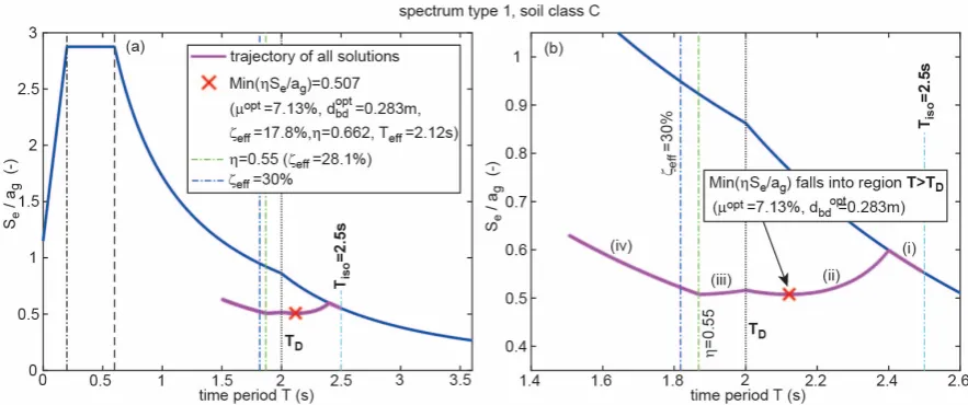
86
• maximum horizontal CSS force:
eff S bd S b R N d N
F =μ + (1)
87
• effective stiffness:
bd b eff
d F
k = (not equal to restoring stiffness NS/Reff) (2)
88
• effective time period:
eff S eff k g N 2
T = π (3)
• effective damping ratio: + μ π μ = ζ eff bd eff R d 2
with constraint ζeff ≤30% (4)
90
• reduction factor:
eff 05 . 0 10 . 0 ζ + =
η with constraints 0.55≤η≤1 (5)
91
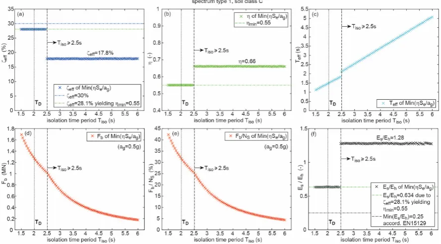
• reduced acceleration response of structure at effective time period: ηSe
(
T=Teff)
(6)92
(acceleration response determined from spectrum and multiplied by η)
93
• maximum horizontal force of structure (single DOF):
g N S
FS =η e S (7)
94
where NS denotes the vertical load in Newton on the CSS, g=9.81 m/s2 is the gravitational field
95
constant, ζeff must not be greater than 30% for linear calculation, the reduction factor η is limited
96
to 1 if ζeff ≤ζS=5% and η≥0.55 limits the reduction of the acceleration response of the structure if
97
>
ζeff 5%. Solving (5) for ζeff with η=0.55 yields ζeff=28.1% (approx.) which shows that the
98
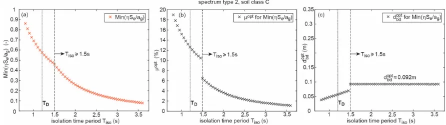
minimum tolerated reduction factor η=0.55 is triggered by ζeff being smaller than its maximum
99
tolerated value of 30% for linear calculation.
100
A valid CSS design is obtained if the maximum horizontal force (1) of the CSS is equal to the
101
maximum horizontal force (7) of the structure (with a reasonable error tolerance). If this condition is
102
not fulfilled the values assumed for μ and dbd must be altered until Fb ≈FS is obtained. As the
103
primary goal of this iterative procedure, which is commonly made by trial and error, is to satisfy
104
S
b F
F ≈ the resulting CSS design – although a valid design – does not necessarily also minimize the
105
acceleration response of the structural. The subsequent section therefore describes a procedure how
106
to obtain all valid CSS designs due to all possible combinations of μ and dbd based on which the
107
CSS design leading to minimum structural acceleration can be identified.
108
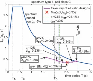
109
Figure 1. Elastic response spectrum including trajectory of all valid CSS designs, limitations due to
110
minimum reduction factor and maximum effective damping ratio and optimum CSS design for minimum
111
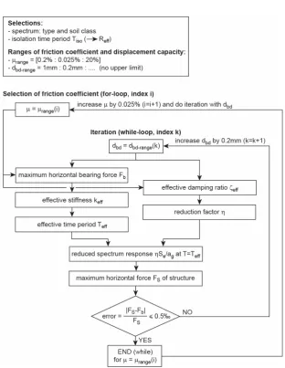
113
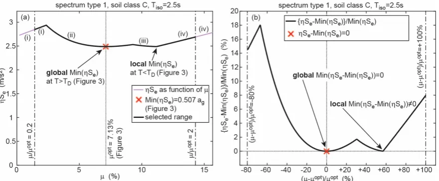
Figure 2. Flow chart of software program to compute all valid CSS designs.
114
2.2. Optimum CSS design for minimum structural acceleration
115
A software program is presented which allows computing any valid CSS design based on
116
different combinations of μ and dbd satisfying Fb ≈FS; Figure 2 depicts the flow chart of this
117
software program. The software program basically consists of a for-loop where μ is selected based
118
on the assumed friction coefficient range μrange beginning at μ=0.2% and ending at μ=20% with
119
increment of 0.025% and a while-loop that computes dbd for the selected μ such that the relative
120
error of Fb ≈FS is not greater than 0.5‰. For the assumed friction coefficient range with 792
121
elements this software program computes 792 valid CSS designs. These valid CSS designs are
122
plotted in the spectrum plane in Figure 1 by their reduced normalized structural acceleration
123
response ηSe/ag versus their effective time period Teff. Due to the small increment in μrange the
124
plotted points of these valid CSS designs appear as a line, i.e. the trajectory of valid CSS designs.
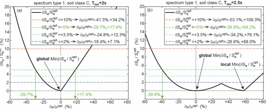
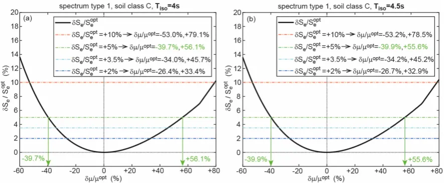
125
Along this trajectory the design parameters μ and dbd of the valid CSS designs change which is
126
shown by some selected valid CSS designs with associated values of μ and dbd. From this
127
trajectory the following can be observed:
128
a) The trajectory of the valid CSS designs starts at Teff ≈Tiso due to the smallest considered
129
friction coefficient μ=0.2% and then primarily propagates to the “left”, i.e. to lower values of
130
eff
T due to the increasing values of μ and the acceleration response of the trajectory is
131
b) As long as ζeff ≤5% the trajectory of the valid CSS designs is congruent with the non-reduced
133
acceleration response of the spectrum because ζeff ≤ζS=5% leads to η=1.
134
c) For 5%<ζeff ≤28.1% the trajectory of the valid CSS designs is below the non-reduced
135
acceleration response of the spectrum because 5%<ζeff ≤28.1% results in 0.55≤η<1.
136
d) To the “left” of the vertical dash-dotted line in green due to ζeff =28.1% and hence η=0.55
137
the reduction factor remains at 0.55 despite ζeff increases up to its maximum tolerated value
138
of 30% due to the increasing μ; ζeff=30% is indicated by the blue vertical dash-dotted line.
139
e) There exists one optimum CSS design that is valid (Fb≈FS) and minimizes the structural
140
acceleration response which is highlighted by the red cross on the trajectory.
141
The optimum CSS design is determined by the described software program after the computation of
142
all valid CSS designs from which the pair of μ and dbd is selected that minimizes the structural
143
acceleration response. In the subsequent section 2.3 and 2.4 the optimum CSS designs are presented
144
for spectra of type 1 and 2 and soil class C; the results due to other soil classes are omitted as their
145
influence on the optimization results is little.
146
2.3. Optimization results for spectrum of type 1 with soil class C
147
2.3.1. Optimum solutions for selected isolation time periods
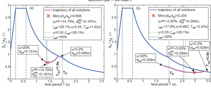
148
Four optimization trajectories due to four selected isolation time periods are presented.
149
Figure 3(a) depicts the case of a rather unrealistically low isolation time period Tiso=1.9 s whereby
150
the entire optimization trajectory lies in the region TC ≤Teff <TD. The optimum CSS design is
151
obtained at minimum tolerated η=0.55 due to ζeff=28.1%, i.e. on the green dash-dotted line. For the
152
more realistic isolation time period Tiso=3.5 s the main part of the optimization trajectory including
153
the optimum CSS design lies in the region Teff ≥TD (Figure 3(b)). The optimum CSS design is
154
characterized by ζeff=17.8% and η=0.662. The optimization trajectory does not show how the state
155
variables μ, dbd, ζeff, η and Teff change along the trajectory. Therefore, the state variables
156
bd
d , ζeff, η and Teff are plotted as function of the varied μ in Figures 4 and 5 for Tiso=1.9 s
157
and Tiso=3.5 s. The force displacement loop of the optimum CSS solution is also included to
158
demonstrate that the optimum CSS design fulfils the re-centring condition Es/Eh ≥0.25.
159
160
Figure 3. Optimization trajectories for (a) Tiso=1.9 s and (b) Tiso=3.5 s for spectrum type 1 with soil
161
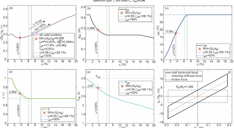
163
Figure 4. (a-e) Optimization results for Tiso=1.9 s as function of friction coefficient and (f) force
164
displacement curve of optimum CSS design for spectrum type 1 with soil class C.
165
166
Figure 5. (a-e) Optimization results for Tiso=3.5 s as function of friction coefficient and (f) force
167
displacement curve of optimum CSS design for spectrum type 1 with soil class C.
168
The location of the optimum CSS design becomes nontrivial when the optimizations are
169
performed for Tiso=1.49 s (Figure 6) and Tiso=1.50 s (Figure 7). For Tiso=1.49 s the optimum CSS
170
design lies in the region Teff <TD because the optimization trajectory, which shows a first local
171
minimum at Teff >TD in section (ii), drops again in section (iii) generating the global minimum at
172
D
eff T
T < (Figure 6(b)). The optimum CSS design is characterized by ζeff=28.1% and η=0.55. In
173
contrast, if Tiso=1.50 s is selected the global minimum is obtained at Teff >TD with ζeff=17.8%
174
176
Figure 6. (a) Optimization trajectory for Tiso=2.49 s and (b) according close-up for spectrum type 1 with
177
soil class C.
178
179
Figure 7. (a) Optimization trajectory for Tiso=2.5 s and (b) according close-up for spectrum type 1 with
180
soil class C.
181
2.3.2. Optimum solutions as function of isolation time period
182
In section 2.3.1 the optimization trajectories with the according optimum CSS designs are
183
shown for some selected isolation time periods, i.e. Tiso=1.9 s, 2.49 s, 2.5 s and 3.5 s. The logical next
184
step is to have a look only at how the optimum CSS design solutions depend on Tiso. Figure 8
185
shows how the optimum design parameters of the CSS, i.e. the optimum friction coefficient μopt
186
and the optimum displacement capacity doptbd , and the resulting minimized structural acceleration
187
response depend on Tiso. The other state variables of interest of the optimum CSS design solutions,
188
i.e. ζeff, η, Teff, Fb/NS and Es/Eh, are depicted in Figure 9 as function of Tiso. The following
189
main observation can be made:
190
• The longer Tiso is the smaller the optimum friction coefficient μopt becomes.
191
• The displacement capacities doptbd of all optimum CSS design solutions whose effective
192
time periods lie in the region Teff >TD are constant because at Teff >TD the reduction
193
factor η=0.66 is constant and ηSe/ag at Teff >TD is in proportion to 1/T2 whereby the
194
according displacement is constant.; notice that doptbd =constant at Teff >TD only applies to
195
• The optimum CSS design in the typical isolation time period region 3.5 s<Tiso<5 s is not
197
obtained from maximum tolerated effective damping ratio ζeff=30% but from the lower
198
value ζeff=17.8% evoking η=0.66.
199
• The jump in the curves of the shown state variables at Tiso=2.5 s is caused by the fact that the
200
optimum CSS design lies in the region Teff <TD if Tiso <2.5 s while it is located in the
201
region Teff >TD if Tiso ≥2.5 s.
202
• Reasonable values for Fb/NS are found in the typical isolation time period region 3.5 s<Tiso
203
<4.5 s.
204
• The re-centring condition Es/Eh ≥0.25 is fulfilled for all optimum CSS design solutions for
205
all considered Tiso.
206
207
Figure 8. (a) Minimum structural acceleration due to optimum selections of (b) friction coefficient and (c)
208
displacement capacity for spectrum type 1 with soil class C.
209
210
Figure 9. States of optimum solution: (a) effective damping ratio, (b) reduction factor, (c) effective time
211
period, (d, e) maximum horizontal CSS force, (f) re-centring condition for spectrum type 1 with soil
212
class C.
213
2.4. Optimization results for spectrum of type 2 with soil class C
214
The optimization trajectories associated by their optimum CSS designs for spectrum type 2 and
215
soil class C are depicted in Figures 10 and 11. Since TD=1.2 s for type 2 is much lower than TD=2 s
216
if Tiso≥1.5 s which explains the jump in the state variables at Tiso=1.5 s (Figures 12 and 13). Similar
218
to the results for spectrum of type 1 not the maximum tolerated effective damping ratio ζeff=30%
219
with associated η=0.55 but ζeff=17.6% with associated η=0.66 minimizes structural acceleration.
220
Also, the re-centring condition is fulfilled for all considered Tiso and shows the same value as for
221
spectrum of type 1.
222
223
Figure 10. Optimization trajectories for (a) Tiso=1 s and (b) Tiso=2 s for spectrum type 2 with soil class C.
224
225
Figure 11. Optimization trajectories for (a) Tiso=1.49 s and (b) Tiso=1.5 s for spectrum type 2 with soil
226
class C.
227
228
Figure 12. (a) Minimum structural acceleration due to optimum selections of (b) friction coefficient and (c)
229
231
Figure 13. States of optimum solution: (a) effective damping ratio, (b) reduction factor, (c) effective time
232
period, (d, e) maximum horizontal CSS force, (f) re-centring condition for spectrum type 2 with soil
233
class C.
234
235
Figure 14. Derivation of sensitivity curves (shown for spectrum type 1 with soil class C and Tiso=2.5 s):
236
(a) reduced acceleration response ηSeas function of friction coefficient μ and (b) according sensitivity
237
curve.
238
3. Sensitivity of friction coefficient on structural acceleration
239
This section describes quantitatively by how much the structural acceleration worsens when the
240
actual friction coefficient of the real CSS deviates from its optimum value minimizing structural
241
acceleration.
242
3.1. Sensitivity formulation
243
The reduced structural acceleration response ηSe computed as function of friction coefficient
244
μ as depicted in Figure 14(a) basically shows by how much the structural acceleration response
245
deteriorates (increases) if the actual friction coefficient of the real CSS deviates (being smaller or
246
system's output (relative change in structural acceleration) for given relative change in the system's
248
input (relative change in friction coefficient). Hence, the sensitivity curve is obtained by, first,
249
subtracting the minimum value from the structural acceleration and the optimum value from the
250
friction coefficient, respectively, and, subsequently, normalizing the first term by its minimum value
251
and the second term by its optimum value (Figure 14(b))
252
{
}
{
}
opt
e e e e e
opt
opt opt
S Min( S ) Min( S ) S / S
sensitivity
/
η − η η δ
= =
δμ μ
μ − μ μ (8)
253
Please note that this sensitivity analysis does not investigate the impact of deviations in μ on
254
the resulting displacement capacity. It is common understanding that a lower actual friction
255
coefficient of the real CSS than its design value will cause larger relative motions in the CSS as, e.g.,
256
visible in Figures 4(b) and 5(b).
257
3.2. Results for spectrum of type 1
258
The sensitivity curves for spectrum of type 1 with soil class C are depicted in Figures 15-17 for
259
the selected isolation time periods Tiso=2 s, 2.5 s, 3 s, 3.5 s, 4 s and 4.5 s. The sensitivity curves for
260
the unusually low Tiso=2 s and 2.5 s are also plotted to demonstrate that structural acceleration is
261
more sensitive to deviations in the actual friction coefficient if Tiso is unusually low (2 s) and that
262
structural acceleration does hardly deteriorate for μ − μopt>0 if Tiso=2.5 s due to the special case that
263
the global and local minima yield a fairly flat sensitivity curve at μ − μopt>0. Horizontal dash-dotted
264
lines in different colours corresponding to different levels of deterioration in δS / Se opte are included
265
in Figures 15-17 to be able to directly read off by how much the actual friction coefficient may
266
deviate (plus and minus) from its optimum value if a certain level of acceptable deterioration in
267
structural acceleration is assumed. For instance the structural engineer may estimate that the
268
structural acceleration may deteriorate by +5% (green dash-dotted line) and then read off directly
269
from the sensitivity curves by how much the actual friction coefficient of the real CSS may differ
270
from its optimum value. For the assumption that δS / Se opte =+5% may be acceptable the sensitivity
271
curves with reasonable isolation time periods Tiso=3 s to 4.5 s demonstrate that the actual friction
272
coefficient of the real CSS may deviate from its optimum value by at least δμ μ/ opt=-39.7% and
273
+55.6%. The tolerances are not symmetric relative to μopt because of the non-symmetrical
274
sensitivity curves.
275
276
277
Figure 15. Sensitivity of deviation in friction coefficient from its optimum value on relative increase of
278
280
Figure 16. Sensitivity of deviation in friction coefficient from its optimum value on relative increase of
281
structural acceleration for (a) Tiso=3 s and (b) Tiso=3.5 s and spectrum of type 1 with soil class C.
282
283
Figure 17. Sensitivity of deviation in friction coefficient from its optimum value on relative increase of
284
structural acceleration for (a) Tiso=4 s and (b) Tiso=4.5 s and spectrum of type 1 with soil class C.
285
Sensitivity curves are also computed for spectrum of type 1 with soil classes A, B, D and E. The
286
results of these computations are evaluated for acceptable deteriorations in δS / Se opte of +5% and
287
+2% and summarized in Table 1 together with the results for spectrum of type 1 with soil class C.
288
This table reveals that – for reasonable isolation time periods Tiso ≥3 s for spectrum of type 1 – the
289
actual friction coefficient of the real CSS may differ from its optimum value by at least δμ μ/ opt
290
=-39.4% and +54.5% if δS / Se opte =+5% may be acceptable and by at least δμ μ/ opt=-26.4% and
291
+32.5% if δS / Se opte =+2% is considered to be acceptable.
292
3.3. Results for spectrum of type 2
293
Analogue to the results for spectrum of type 1 the sensitivity curves for spectrum of type 2 with
294
soil class C are graphically presented (Figures 18-20) and all sensitivities resulting from spectrum of
295
type 2 with all soil classes evaluated at δSe/Sopte =+5% and +2% are summarized in Table 2. For
296
reasonable Tiso≥1.8 s it is seen that the actual friction coefficient of the real CSS may differ from its
297
optimum value by at least δμ μ/ opt=-39.7% and +54.5% assuming δS / Se opte =+5% is acceptable and
298
are very similar to those for spectrum of type 1 because the relative deterioration of the structural
300
acceleration depends on the relative change of the friction coefficient.
301
Table 1. Sensitivity results for spectrum of type 1 for relative increase of +5% and +2% in structural
302
acceleration.
303
iso
T (s) soil class δSe/Sopte δμ/μopt δSe/Sopte δμ/μopt
2
A +5% -29.6%, +17.7% 2% -18.3%, +7.3%
B +5% -29.7%, +17.4% 2% -18.4%, +7.0%
C +5% -29.7%, +17.4% 2% -18.4%, +7.1%
D +5% -29.6%, +17.5% 2% -18.3%, +7.1%
E +5% -29.6%, +17.6% 2% -18.3%, +7.2%
2.5
A +5% -39.8%, +84.4% 2% -26.6%, +68.1%
B +5% -39.9%, +84.0% 2% -26.7%, +67.8%
C +5% -39.9%, +84.2% 2% -26.6%, +68.0%
D +5% -39.9%, +84.1% 2% -26.7%, +67.9%
E +5% -39.9%, +84.2% 2% -26.7%, +67.9%
3
A +5% -40.0%, +55.2% 2% -26.9%, +32.7%
B +5% -39.8%, +55.7% 2% -26.6%, +33.0%
C +5% -39.9%, +55.6% 2% -26.7%, +32.9%
D +5% -39.9%, +55.5% 2% -26.7%, +32.8%
E +5% -40.0%, +55.4% 2% -26.8%, +32.8%
3.5
A +5% -39.7%, +56.2% 2% -26.4%, +33.4%
B +5% -39.7%, +56.1% 2% -26.4%, +33.4%
C +5% -39.7%, +56.1% 2% -26.4%, +33.4%
D +5% -40.0%, +55.3% 2% -26.8%, +32.7%
E +5% -40.1%, +55.1% 2% -26.9%, +32.5%
4
A +5% -40.3%, +54.5% 2% -27.2%, +32.0%
B +5% -40.0%, +55.2% 2% -26.8%, +32.7%
C +5% -39.7%, +56.1% 2% -26.4%, +33.4%
D +5% -39.8%, +55.8% 2% -26.6%, +33.1%
E +5% -39.9%, +55.5% 2% -26.7%, +32.8%
4.5
A +5% -39.9%, +55.6% 2% -26.6%, +32.9%
B +5% -39.5%, +56.6% 2% -26.2%, +33.8%
C +5% -39.9%, +55.6% 2% -26.7%, +32.9%
D +5% -40.0%, +55.2% 2% -26.8%, +32.6%
E +5% -39.7%, +56.0% 2% -26.5%, +33.3%
5
A +5% -39.4%, +56.7% 2% -26.1%, +33.9%
B +5% -39.9%, +55.4% 2% -26.7%, +32.8%
C +5% -39.7%, +56.1% 2% -26.4%, +33.4%
D +5% -40.2%, +54.9% 2% -27.0%, +32.3%
E +5% -39.6%, +56.2% 2% -26.4%, +33.4%
306
Figure 18. Sensitivity of deviation in friction coefficient from its optimum value on relative increase of
307
structural acceleration for (a) Tiso=1.2 s and (b) Tiso=1.5 s and spectrum of type 2 with soil class C.
308
309
Figure 19. Sensitivity of deviation in friction coefficient from its optimum value on relative increase of
310
structural acceleration for (a) Tiso=1.8 s and (b) Tiso=2.1 s and spectrum of type 2 with soil class C.
311
312
Figure 20. Sensitivity of deviation in friction coefficient from its optimum value on relative increase of
313
structural acceleration for (a) Tiso=2.4 s and (b) Tiso=2.7 s and spectrum of type 2 with soil class C.
314
Table 2. Sensitivity results for spectrum of type 2 for relative increase of +5% and +2% in structural
316
acceleration.
317
iso
T (s) soil class δSe/Sopte δμ/μopt δSe/Sopte δμ/μopt
1.2
A +5% -29.7%, +17.6% 2% -18.3%, +7.1%
B +5% -29.7%, +17.5% 2% -18.4%, +7.1%
C +5% -29.7%, +17.4% 2% -18.4%, +7.1%
D +5% -29.6%, +17.6% 2% -18.3%, +7.2%
E +5% -29.7%, +17.4% 2% -18.4%, +7.1%
1.5
A +5% -39.9%, +84.1% 2% -26.7%, +67.9%
B +5% -39.8%, +84.4% 2% -26.6%, +68.2%
C +5% -39.8%, +84.3% 2% -26.6%, +68.0%
D +5% -39.9%, +84.0% 2% -26.7%, +67.8%
E +5% -39.8%, +84.3% 2% -26.6%, +68.1%
1.8
A +5% -39.7%, +56.2% 2% -26.4%, +33.5%
B +5% -39.7%, +55.9% 2% -26.5%, +33.2%
C +5% -39.8%, +55.9% 2% -26.6%, +33.1%
D +5% -39.9%, +55.6% 2% -26.6%, +33.0%
E +5% -39.8%, +55.8% 2% -26.6%, +33.1%
2.1
A +5% -40.0%, +55.2% 2% -26.9%, +32.5%
B +5% -40.1%, +55.0% 2% -27.0%, +32.4%
C +5% -40.0%, +55.3% 2% -26.8%, +32.6%
D +5% -40.0%, +55.3% 2% -26.8%, +32.7%
E +5% -39.7%, +56.2% 2% -26.4%, +33.4%
2.4
A +5% -39.7%, +56.0% 2% -26.5%, +33.3%
B +5% -40.0%, +55.2% 2% -26.8%, +32.6%
C +5% -40.0%, +55.4% 2% -26.8%, +32.7%
D +5% -39.8%, +55.8% 2% -26.6%, +33.1%
E +5% -40.1%, +55.0% 2% -27.0%, +32.4%
2.7
A +5% -39.8%, +55.7% 2% -26.6%, +33.1%
B +5% -40.1%, +54.9% 2% -27.0%, +32.4%
C +5% -40.1%, +55.0% 2% -27.0%, +32.4%
D +5% -40.0%, +55.2% 2% -26.9%, +32.6%
E +5% -39.9%, +55.6% 2% -26.7%, +32.9%
3
A +5% -39.9%, +55.6% 2% -26.6%, +32.9%
B +5% -39.8%, +55.8% 2% -26.5%, +33.2%
C +5% -40.3%, +54.5% 2% -27.2%, +32.0%
D +5% -39.9%, +55.5% 2% -26.7%, +32.8%
E +5% -40.0%, +55.3% 2% -26.8%, +32.7%
318
4. Summary and conclusions
319
This paper first presents an optimization routine that derives all valid designs of curved surface
320
sliders (CSS) based on the method of the linear response spectrum. All valid CSS designs are
321
represented by their acceleration trajectory in the elastic response spectrum plane. The fairly flat
322
minimum of the acceleration trajectory reveals that deviations in the actual friction coefficient of the
323
real CSS from its optimum value do not have great deteriorating impact on structural acceleration.
324
The second part of this study describes how friction coefficient, displacement capacity, effective
325
damping ratio, reduction factor, effective time period and re-centring condition of all optimum CSS
326
reasonable isolation time periods demonstrate that the optimum CSS, which minimizes structural
328
acceleration, is not obtained at maximum tolerated effective damping ratio of 30% of the CSS but at a
329
significantly lower value.
330
The third and final part of the paper is concerned with the question by how much the structural
331
acceleration deteriorates when the actual friction coefficient of the real CSS differs from its optimum
332
value. The underlying sensitivity analysis, which is performed for spectra of type 1 and 2 and all soil
333
classes, demonstrates that the relative increase in the structural acceleration is approximately one
334
order of magnitude smaller than the assumed deviation in the actual friction coefficient from its
335
optimum value. The sensitivity results may be used by the structural engineer to define tolerable
336
deviations in the actual friction coefficient from its optimum value such that the resulting structural
337
acceleration response is still acceptably small.
338
Acknowledgments: The authors gratefully acknowledge the financial supports of Maurer Switzerland GmbH,
339
Zurich, Switzerland, MAURER ENEGINEERING GmbH, Munich, Germany, and MAURER SE, Munich,
340
Germany.
341
Author Contributions: Felix Weber, Leopold Meier and Johann Distl performed the optimization analysis;
342
Felix Weber and Christian Braun made the sensitivity analysis; all authors were involved in writing the paper.
343
Conflicts of Interest: The authors declare no conflict of interest.
344
References
345
1. Yen, K.Z.Y., Lee Y.J. Passive vibration isolating system. US Patent No. 6126136, October 3, 2000.
346
2. Eurocode 8: Design of structures for earthquake resistance – Part 1: General rules, seismic actions and
347
rules for buildings, EN 1998-1:2004 + AC:2009.
348
3. Lai, M.L., Soong, T.T. Seismic design considerations for secondary structural systems. Journal of Structural
349
Engineering (United States) 1991; 117, 459-472.
350
4. Inaudi, J.A., Kelly, J.M. Optimum damping in linear isolation systems. Earthquake Engineering & Structural
351
Dynamics 1993, 22, 583-598.
352
5. Kelly, J.M. The role of damping in seismic isolation. Earthquake Engineering and Structural Dynamics1999,
353
28, 3-20.
354
6. Hall, J.F., Discussion: the role of damping in seismic isolation. Earthquake Engineering and Structural
355
Dynamics 1999, 28, 1717-1720.
356
7. Du, Y., Zhao, G. Analysis of effect of non-classical damping on isolated structure and optimum damping.
357
Journal of Earthquake Engineering and Engineering Vibration2000, 20, 100-107.
358
8. Jangid, R.S. Optimum friction pendulum system for near-fault motions. Engineering Structures2005, 27,
359
349-359.
360
9. Bucher, C. Probability-based optimization of friction damping devices. Structural Safety2009, 31, 500-507.
361
10. Kovaleva, N.V., Rutman, Yu.L., Davydova, G.V. Determination of optimal damping parameters for
362
seismic isolation systems. Magazine of Civil Engineering2013, 40, 107-115.
363
11. Nigdeli, S.M., Bekdaş, G., Alhan, C. Optimization of seismic isolation systems via harmony search.
364
Engineering Optimization2014, 46, 1553-1569.
365
12. Kamalzare, M., Johnson, E.A., Wojtkiewicz, S.F. Efficient optimal design of passive structural control
366