Mech. Sci., 4, 233–242, 2013 www.mech-sci.net/4/233/2013/ doi:10.5194/ms-4-233-2013
©Author(s) 2013. CC Attribution 3.0 License.
Mechanical
Sciences
Open Access
Internal redundancy: an approach to improve the
dynamic parameters around sharp corners
S. S. Parsa1, J. A. Carretero1, and R. Boudreau2
1Department of Mechanical Engineering, University of New Brunswick, Fredericton, NB, Canada
2D´epartement de g´enie m´ecanique, Universit´e de Moncton, Moncton, NB, Canada
Correspondence to: J. A. Carretero ([email protected])
Received: 11 December 2012 – Revised: 8 March 2013 – Accepted: 5 April 2013 – Published: 28 May 2013
Abstract. In recent years, redundancy in parallel manipulators has been studied broadly due to its capabil-ity of overcoming some of the drawbacks of parallel manipulators including small workspaces and singular configurations. Internal redundancy, first introduced for serial manipulators, refers to the concept of adding movable masses to some links so as to allow to control the location of the centre of mass and other dynamic properties of some links. This concept has also been referred to as variable geometry. This paper investigates the effects of internal redundancy on the dynamic properties of a planar parallel manipulator while performing a family of trajectories. More specifically, the 3-RRR planar manipulator, where a movable mass has been added to the distal link, is allowed to trace trajectories with rounded corners and different radii. The proposed method uses the manipulator’s dynamic model to actively optimise the location of the redundant masses at every point along the trajectory to improve the dynamic performance of the manipulator. Numerical examples are shown to support the idea.
1 Introduction
Redundancy in parallel manipulators is normally divided into kinematic redundancy, actuation redundancy and branch re-dundancy (Lee and Kim, 1993; Zanganeh and Angeles, 1994; Merlet, 1996; Ruggiu and Carretero, 2009; Boudreau and Nokleby, 2012). Actuation redundancy consists of replac-ing passive joints with active ones (Zanganeh and Angeles, 1994; Cheng et al., 2003, 2011; Nokleby et al., 2005) where the number of degrees-of-freedom or mobility of the manip-ulator does not change. Although actuation redundancy can help either eliminate or reduce singular configurations, is-sues such as force interference make the manipulators more complex to analyze, design and control (Firmani and Pod-horodeski, 2004; Garg et al., 2009). The second type of re-dundancy is called branch rere-dundancy where an extra ac-tuated branch is added to the manipulator (Firmani et al., 2007). Branch redundancy can improve the force capabili-ties of the manipulator and reduce the number of singular configurations. The third type of redundancy is called kine-matic redundancy where active joints and links are added
to one or more branches of the manipulator (Merlet, 1996; Wang and Gosselin, 2004). This type of redundancy can en-hance the dexterity of the manipulator as well as enlarge the workspace. Additionally, kinematic redundancy allows to plan trajectories far from certain singular configurations as the inverse displacement problem has an infinite number of solutions (thus often allowing for the manipulator to remain as far as possible from singular configurations) (Ebrahimi et al., 2008).
Redundant parallel manipulators have been widely used to improve the trajectories of parallel robots. For instance, Cha et al. (2007) showed that kinematically redundant manipu-lators can effectively avoid singular configurations thus in-creasing the singularity-free workspace of the parallel ma-nipulator.
234 S. S. Parsa et al.: Internal redundancy to improve dynamic parameters in corners 2 S. S. Parsa, J. A. Carretero and R. Boudreau: Internal Redundancy to Improve Dynamic Parameters in Corners
A
P
B φ
s
θ1 θ2
φ x y l1
l2
lm2
m1
ms
m3
me
C θ3
lm1
m2
l3 lm3
link 1 link 2
link 3
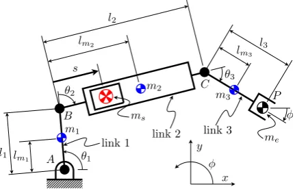
Fig. 1:Serial manipulator with internal redundancy in link2. The location of massmscan be changed without altering the position
of the end effector (pointp).
degrees of freedom (DOF) is added to the serial manipula-tor. However, in contrast with the redundant actuators and/or links described earlier, the new DOF is used to change the internal geometry of a link resulting in the change of the lo-cation of the link’s centre of mass and its inertial mass dis-tribution parameters (i.e., its mass moment of inertia). Since the changes are made within the internal members of the link, the redundant DOF does not have a direct effect on the end effector pose (i.e., position and orientation). More specifi-cally, in reference to Figure 1, the position of the massmsin
link 2 can be changed without altering the pose of the end ef-fector. This allows for different internal motions for a given trajectory of the end effector thus adding control to some dy-namic parameters of the manipulator to attempt to improve its dynamic performance for specific tasks.
In this paper, the concept of internal redundancy is applied to a planar parallel manipulator. First, a 3-RRR manipulator with internal redundancy in all three branches is described and its kinematic and dynamic equations (Sections 2 and 3) are derived. Then, an optimisation problem is formulated where the displacement of each of the portable masses at ev-ery point throughout a trajectory is sought to minimise the torques at the base actuators (Section 4). The architectural parameters and trajectory planning algorithm are explained through a numerical example and are presented in Section 5 and then discussed in more detail in Section 6. Finally, Sec-tion 7 presents the conclusions and briefly discusses potential future work.
2 The 3-RRR Manipulator with Internal Redundancy
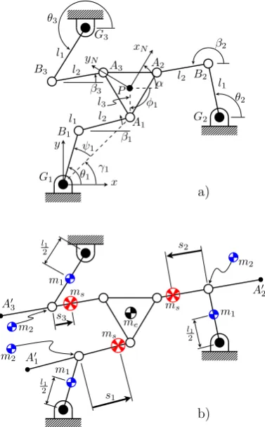
A 3-DOF planar parallel manipulator shown in Figure 2a is chosen to investigate the effect of internal redundancy in parallel manipulators. The manipulator is a symmetrical 3-RRR manipulator with base (G1G2G3) and end effector (A1A2A3) as equilateral triangles. The three revolute actu-ators to move the manipulator’s end effector are located at
Gi, the base joint of each branch. The length of the
proxi-mal links,i.e., linksGiBi(i= 1,2,3), has been denoted byl1 while the length of the distal link,i.e.,BiAi (i= 1,2,3) has
been denoted byl2.
In order to study the concept of internal redundancy, a por-tion of the distal link (the porpor-tion fromBi toA0i) protrudes
on the opposite side of the revolute joint atBi and creates
a linear track fromAi toA0iwhere the redundant massms
can slide on (see Figure 2b). The position of the mass rela-tive to the elbow jointBi is given bysiand is measured in
the direction ofAi. Since the masses ms are mounted on
tracks or prismatic joints, their position alongAiA0i can be
actively controlled. More specifically, the distancesi from
elbow jointBito the centre of massmscan be actively
con-trolled thus changing the overall dynamic properties and ef-fects of linksA0iAi.
To help complete the dynamic model, each element has been given a mass while symmetry has been assumed to sim-plify the analysis. Moreover, the links have been modelled as slender rods. The proximal links have all been assigned a massm1with their centre of mass located halfway between
Giand Bi while all three distal links have been assigned a
massm2with their centre of mass located halfway between
A0iandAi. The moving platform has been assigned a mass
mewith its barycentre located at the centroid of the moving
platform.
3 Dynamic Model of the Redundant 3-RRR Manipula-tor
The inverse dynamic problem of a 3-RRR planar parallel ma-nipulator with 3-DOF of internal redundancy is developed in this section. The dynamic model is obtained using the Prin-ciple of Virtual Work as well as d’Alembert’s prinPrin-ciple. The derivation is similar to that presented in Wu et al. (2011). For this purpose, a complete kinematic model of the manipulator needs to be developed to derive the velocity and acceleration equations. In addition to that, inertial forces and moments of all the links need to be calculated.
Note that in what follows, the equations are derived for each of the three legs. Therefore, indexi in the equations that follow is assumed to respectively take the values 1, 2 and 3 when deriving the equations for legs 1, 2 and 3.
3.1 Kinematics
The base coordinate frameO-xy(denoted by{O}) shown in Figure 2 is fixed on pointG1. Also, a moving coordinate frameP-xNyN (denoted by{N}) is attached to the
barycen-tre of the moving platform. The position vector ofBiin the
base coordinate frame is defined as follows:
rBi=rGi+l1
cosθi sinθi
(1)
Figure 1.Serial manipulator with internal redundancy in link 2.
The location of mass mscan be changed without altering the
posi-tion of the end effector (point p).
the actuated joints on the kinematically redundant manipu-lator are significantly less than the ones needed for a non-redundant manipulator.
Recently, a new type of redundancy called internal redun-dancy has been the focus of some attention in the context of serial manipulators (Vukobratovi´c et al., 2000). Similar to the types of redundancy described earlier, a new set of degrees of freedom (DOF) is added to the serial manipulator. How-ever, in contrast with the redundant actuators and/or links de-scribed earlier, the new DOF is used to change the internal geometry of a link resulting in the change of the location of the link’s centre of mass and its inertial mass distribution pa-rameters (i.e., its mass moment of inertia). Since the changes are made within the internal members of the link, the redun-dant DOF does not have a direct effect on the end effector pose (i.e., position and orientation). More specifically, in ref-erence to Fig. 1, the position of the mass msin link 2 can be changed without altering the pose of the end effector. This allows for different internal motions for a given trajectory of the end effector thus adding control to some dynamic param-eters of the manipulator to attempt to improve its dynamic performance for specific tasks.
In this paper, the concept of internal redundancy is ap-plied to a planar parallel manipulator. First, a 3-RRR ma-nipulator with internal redundancy in all three branches is described and its kinematic and dynamic equations (Sects. 2 and 3) are derived. Then, an optimisation problem is formu-lated where the displacement of each of the portable masses at every point throughout a trajectory is sought to minimise the torques at the base actuators (Sect. 4). The architectural parameters and trajectory planning algorithm are explained through a numerical example and are presented in Sect. 5 and then discussed in more detail in Sect. 6. Finally, Sect. 7 presents the conclusions and briefly discusses potential fu-ture work.
2 The 3-RRR manipulator with internal redundancy
A 3-DOF planar parallel manipulator shown in Fig. 2a is cho-sen to investigate the effect of internal redundancy in parallel manipulators. The manipulator is a symmetrical 3-RRR ma-nipulator with base (G1G2G3) and end effector (A1A2A3) as equilateral triangles. The three revolute actuators to move the manipulator’s end effector are located at Gi, the base joint of each branch. The length of the proximal links, i.e., links GiBi (i=1,2,3), has been denoted by l1 while the length of the distal link, i.e., BiAi(i=1,2,3) has been denoted by l2.
In order to study the concept of internal redundancy, a por-tion of the distal link (the porpor-tion from Bito A0i) protrudes on the opposite side of the revolute joint at Biand creates a lin-ear track from Aito A0iwhere the redundant mass mscan slide on (see Fig. 2b). The position of the mass relative to the el-bow joint Biis given by siand is measured in the direction of
Ai. Since the masses msare mounted on tracks or prismatic joints, their position along AiA0i can be actively controlled. More specifically, the distance sifrom elbow joint Bito the centre of mass ms can be actively controlled thus changing the overall dynamic properties and effects of links A0iAi.
To help complete the dynamic model, each element has been given a mass while symmetry has been assumed to sim-plify the analysis. Moreover, the links have been modelled as slender rods. The proximal links have all been assigned a mass m1 with their centre of mass located halfway between
Gi and Bi while all three distal links have been assigned a mass m2 with their centre of mass located halfway between
A0
i and Ai. The moving platform has been assigned a mass
mewith its barycentre located at the centroid of the moving platform.
3 Dynamic model of the redundant 3-RRR manipulator
The inverse dynamic problem of a 3-RRR planar parallel ma-nipulator with 3-DOF of internal redundancy is developed in this section. The dynamic model is obtained using the Prin-ciple of Virtual Work as well as d’Alembert’s prinPrin-ciple. The derivation is similar to that presented in Wu et al. (2011). For this purpose, a complete kinematic model of the manipulator needs to be developed to derive the velocity and acceleration equations. In addition to that, inertial forces and moments of all the links need to be calculated.
Note that in what follows, the equations are derived for each of the three legs. Therefore, index i in the equations that follow is assumed to respectively take the values 1, 2 and 3 when deriving the equations for legs 1, 2 and 3.
3.1 Kinematics
The base coordinate frame O-xy (denoted by{O}) shown in Fig. 2 is fixed on point G1. Also, a moving coordinate frame
S. S. Parsa et al.: Internal redundancy to improve dynamic parameters in corners 235 S. S. Parsa, J. A. Carretero and R. Boudreau: Internal Redundancy to Improve Dynamic Parameters in Corners 3
A2 A3 A1 G2 G3 G1 P B3 B1 B2 α s2 s3 s1 θ1 θ2 θ3
l1 l2 l1 l2 l1 l2 l1 2 l1 2 l1 2 m1 m1 m1 m2 ms ms
m2 m
s m2 me x y a) b) β2 β1 β3 xN yN l3 γ1 ψ1 φ1 A′ 2 A′ 3 A′ 1
Fig. 2: 3-RRR planar manipulator: a) basic kinematic parameters and b) location of the centre of mass of each component (liare fixed
values whilesiare variable).
whererBi describes the position vector of pointBi,rGi is the position vector of pointGiandθiis the angle linkGiBi
makes with thexaxis (i.e., the actuation variable for the mo-tor located atGi). The position vector ofAiis expressed as
follows:
rAi=rBi+l2
cosβi sinβi
=rp+RrNAi (2)
whererAiis the position vector of pointAi,βidescribes the angle of linkBiAiwith respect to the horizontalxdirection,
rp is the position vector of pointp and rNAi is the position vector ofAi expressed in frameN. The rotation matrixR
describing frame {N} relative to frame{O} is defined as follows:
R=
cosα−sinα
sinα cosα
. (3)
The constraint equation of motion is written as follows:
krAi−rBik=l2 (4)
wherel2is the portion of the distal link fromBitoAi.
3.2 Inverse Displacement Problem
The inverse displacement problem of the 3-RRR planar ma-nipulator is written as follows:
θi=γi±ψi (5)
whereγiis defined as follows:
γi=atan2(xAi,yAi) (6)
where atan2 is the quadrant corrected inverse tangent func-tion. whilexAiandyAiare the Cartesian components of the position ofAirelative toGiand are written as follows:
xAi =x−l3cosφi−xGi (7) yAi =y−l3sinφi−yGi (8)
where xandy are Cartesian positions of pointP,l3is the radius of the moving platform (i.e., the distance betweenP andAi) andφiis given by
φ1=α+
π
6 φ2=α+ 5π
6 φ3=α−
π
2. (9)
The equation forψiis written as follows:
ψi= cos−1 l2
1−l22+x2Ai+y 2
Ai
2l1(x2Ai+y 2
Ai)
. (10)
3.3 Velocity and Acceleration
Taking the time derivative of equation (1) leads to
˙
rBi=l1θ˙i
−sinθi cosθi
(11)
where θ˙i is the angular velocity of actuator i. The linear
velocity of pointAiis written as follows:
˙
rAi=vP+ ˙αNRr
N
Ai= ˙rBi+l2β˙i
−sinβi cosβi
(12)
wherevPis the vector describing the linear velocity of point
P. MatrixNis defined as follows:
N=
0−1 1 0
. (13)
The angular velocity of linkBiAi is derived from
equa-tion (12) and is written as follows:
˙
βi=
−sinβi
l2
cosβi
l2
(˙rAi−r˙Bi) (14)
The linear acceleration of pointsBiandAiis obtained as
the time derivative of equations (11) and (12):
aBi =l1θ¨i
−sinθi cosθi
−l1θ˙i2
cosθi sinθi
(15)
aAi =aP+ ¨αNRr
N
Ai−α˙
2RrN
Ai (16)
Figure 2.3-RRR planar manipulator: (a) basic kinematic
parame-ters and (b) location of the centre of mass of each component (liare
fixed values while siare variable).
moving platform. The position vector of Biin the base coor-dinate frame is defined as follows:
rBi=rGi+l1
"
cosθi sinθi
#
(1)
where rBi describes the position vector of point Bi, rGiis the position vector of point Giandθiis the angle link GiBimakes with the x-axis (i.e., the actuation variable for the motor lo-cated at Gi). The position vector of Aiis expressed as follows:
rAi=rBi+l2
"
cosβi sinβi
#
=rp+RrNAi (2)
where rAi is the position vector of point Ai,βidescribes the angle of link BiAiwith respect to the horizontal x direction,
rp is the position vector of point p and rNAi is the position vector of Aiexpressed in frame N. The rotation matrix R de-scribing frame{N}relative to frame{O}is defined as follows:
R=
"
cosα −sinα sinα cosα
#
. (3)
The constraint equation of motion is written as follows:
krAi−rBik=l2 (4)
where l2is the portion of the distal link from Bito Ai.
3.2 Inverse displacement problem
The inverse displacement problem of the 3-RRR planar ma-nipulator is written as follows:
θi=γi±ψi (5)
whereγiis defined as follows:
γi=atan2 xAi,yAi
(6)
where atan2 is the quadrant corrected inverse tangent func-tion, while xAi and yAi are the Cartesian components of the position of Airelative to Giand are written as follows:
xAi = x−l3cosφi−xGi (7)
yAi = y−l3sinφi−yGi (8)
where x and y are Cartesian positions of point P, l3 is the radius of the moving platform (i.e., the distance between P and Ai) andφiis given by
φ1=α+
π
6 φ2=α+ 5π
6 φ3=α−
π
2. (9)
The equation forψiis written as follows:
ψi=cos−1
l2
1−l 2 2+x
2 Ai+y
2 Ai 2l1(x2Ai+y2Ai)
. (10)
3.3 Velocity and acceleration
Taking the time derivative of Eq. (1) leads to
˙rBi=l1θ˙i
"
−sinθi cosθi
#
(11)
where ˙θi is the angular velocity of actuator i. The linear ve-locity of point Aiis written as follows:
˙rAi=vP+α˙NRr N
Ai=˙rBi+l2β˙i
"
−sinβi cosβi
#
(12)
where vPis the vector describing the linear velocity of point
P. Matrix N is defined as follows:
N=
"
0 −1
1 0
#
. (13)
The angular velocity of link BiAiis derived from Eq. (12) and is written as follows:
˙
βi=
"
−sinβi
l2
cosβi
l2
#
˙rAi−˙rBi
(14)
The linear acceleration of points Biand Aiis obtained as the time derivative of Eqs. (11) and (12):
aBi = l1θ¨i
"
−sinθi cosθi
#
−l1θ˙i2
"
cosθi sinθi
#
(15)
aAi = aP+α¨NRr N Ai−α˙
2RrN
236 S. S. Parsa et al.: Internal redundancy to improve dynamic parameters in corners where aP is the linear acceleration of point P. The time
derivative of Eq. (14) leads to
¨
βi=
"
−sinβi
l2
cosβi
l2
#
aAi−aBi
−β˙
"
cosβi
l2
sinβi
l2
#
˙rAi−˙rBi
. (17)
In order to generate the Jacobian matrix, the time deriva-tive of Eq. (4) yields
J=
−a1
c1 −b1
c1 −d1
c1 −a2
c2 −b2
c2 −d2
c2 −a3
c3 −b3
c3 −d3
c3
(18)
where the elements of this Jacobian matrix are as follows:
ai = −h1(x−xGi)+h3cosθi+h1cosφi (19)
bi = −h1(y−yGi)+h1sinθi+h2sinφi (20)
ci = h3[(y−yGi) cosθi−(x−xGi) sinθi] (21) +sin(θi−φi)
di = h2[(y−yGi) cosφi−(x−xGi) sinφi] (22)
−sin(θi−φi)
where xGi and yGi are the Cartesian components of the posi-tion of point Gi(Gosselin and Angeles, 1988) while h1=l1
1l3, h2=l1
1 and h3=
1 l3.
3.4 Link Jacobian matrices
Since the Principle of Virtual Work is applied to develop the dynamic model of the 3-RRR manipulator, link Jacobian ma-trices have to be derived. When the end effector is subjected to a virtual displacement, the link Jacobian sub-matrix re-lated to the linear velocity provides the virtual displacement of a point on a link, while the link Jacobian sub-matrix re-lated to angular velocity produces the virtual angular dis-placement of a link (also referred to as partial velocity and partial angular velocity matrices by some authors, Wu et al., 2009, 2011). Points Gi, Biand P are considered as the pivotal points of links GiBi, BiAi and the moving platform, respec-tively. The link Jacobian sub-matrix related to the angular velocity of link GiBiis written as follows:
Gi1=
h−ai
ci
−bi ci
−di ci
i
. (23)
The link Jacobian sub-matrix related to the linear velocity of point Gi is zero since the velocity of that point is zero. The link Jacobian sub-matrix related to the linear velocity of point Giis thus written as:
Hi1=0 (24)
The link Jacobian sub-matrix related to the linear velocity of point Bi and the link Jacobian sub-matrix related to the
angular velocity of link BiAi are obtained from J (Eq. 18) and from Eq. (14), respectively and are written as follows:
Hi2 =
l1
ci
"
aisinθi bisinθi disinθi −aicosθi −bicosθi −dicosθi
#
(25)
Gi2 =
h−sinβi
l2
cosβi l2
i h
e1 e2
i
+NRrAie T 3
−
"
−l1sinθi
l1cosθi
# Gi1
!
(26)
where e1=[1 0 0]T, e2=[0 1 0]Tand e3=[0 0 1]T. The link Jacobian sub-matrix related to the angular veloc-ity of the moving platform and the link Jacobian sub-matrix related to the linear velocity of point P are written as follows:
GN = eT3 (27)
HN =
"
1 0 0
0 1 0
#
. (28)
3.5 Inertial force and inertial moment
Here, the Newton-Euler formulation is applied to develop the inertial forces and the inertial moments of each moving body about its centre of mass. Then, these inertial forces and mo-ments are calculated about pivotal points (i.e., points Ai,Bi and Gi). The inertial force and moment of link GiBi about pivotal point Giare written as follows:
Fi1 = −m1
l1 2 ¨
θi[−sinθi cosθi]T
−l1 2θ˙
2
i[cosθi sinθi]T
!
(29)
Mi1 = −θ¨iIi1 (30)
whereθi, ˙θiand ¨θiare the angular displacement, angular ve-locity and angular acceleration of actuator i, and Ii1 is the moment of inertia of link GiBiabout point Gi.
The influence of internal redundancy appears in the iner-tial force and moment of the distal links where the moment of inertia and mass centre of the links vary with respect to the position of ms. The equations for the inertial force and mo-ment about point Biof the distal links are written as follows:
Fi2=−m2tot
aBi+ri2β¨i
−sinβ
icosβi T
−ri2β˙2i
cosβ
isinβiT
−mss¨icosβi sinβiT
−2ms˙siβ˙i−sin(βi) cos(βi)T (31)
Mi2=−β¨iIi2−m2totri2−sinβi cosβiaBi
−2mssi˙siβ˙i (32)
whereβi, ˙βiand ¨βiare the displacement, angular velocity and angular acceleration of the passive joints and m2totis the total mass of link A0
iAi, i.e., m2tot=m2+ms. Also, aBidescribes the linear acceleration of point Bi, ri2is the distance between the centre of mass of link A0
S. S. Parsa et al.: Internal redundancy to improve dynamic parameters in corners 237 is siwhile ˙siand ¨sidescribe the velocity and acceleration of
ms. The position of the centre of mass of the distal link and its moment of inertia vary with respect to the position of the portable mass and are written as follows:
ri2 =
mssi+m2rG2 m2+ms
(33)
Ii2 = IA0
iAi+ms(si)
2 (34)
where rG2 is the position of the centre of mass of the distal
link (excluding ms) and is equal to zero for the case when
BiAi is equal to BiA0i, and IA0
iAi is the moment of inertia of link A0iAiabout its centre of mass (excluding ms).
The inertial force and moment of the moving platform about point P is written as follows:
FN = −mnaP (35)
MN = −α¨IN (36)
where aP and ¨αare the linear acceleration of point P and the angular acceleration of the moving platform, respectively while mnand INrepresents the mass and the moment of iner-tia of the moving platform.
3.6 Dynamic model
The dynamic equation of the 3-RRR is written as follows:
JTτ +
3
X
i=1 2
X
j=1
h
HTi j GTi ji hFi j Mi j
iT
+ h
HTN GTNi[FN MN]T=0 (37)
where J is the Jacobian matrix of the manipulator,τpresents the torque vector, Hi j are the link Jacobian sub-matrices re-lated to velocity and Gi j are the link Jacobian sub-matrices related to the angular velocity of the links, HNand GN repre-sent the link Jacobian sub-matrix related to velocity and the link Jacobian sub-matrix related to the angular velocity of the moving platform, Fi jand Mi jare inertial forces and mo-ments of the robot links and FNand GNrepresent the inertial force and moment of the moving platform.
4 Trajectory optimisation
When planning a trajectory in the Cartesian space, the dis-placement, velocity and acceleration of the end effector are known. These can be used to calculate the kinematic proper-ties of all active joints for every point in the trajectory while the dynamic equations can be used to compute the actuator torques. Since the necessary torques to move the end effector are a function of the position, velocity and acceleration of the portable masses, moving the redundant masses (i.e., chang-ing si, ˙siand ¨sifor i=1,2,3) will also have a direct effect on the torques at the base-mounted actuators.
Here, variables siare optimised to minimise the manipula-tor’s total torque at a specific time step within the trajectory.
The optimisation problem is written as follows:
min si
3
X
i=1
(τi(si)−λτ¯i)2 (38)
subject to −l2≤si≤l2 (39)
−˙smax≤˙si≤˙smax (40)
−¨smax≤¨si≤¨smax (41)
whereτi refers to the optimised torque of actuator i at ev-ery time step, ¯τiis the torque value obtained when a similar manipulator without internal redundancy is used andλis a coefficient between 0 and 1 which makes the objective func-tion flexible on the percentage of the optimised torque value with respect to the torques of the non-redundant manipula-tor. The optimisation variable (i.e., si) is the distance from joint Bito the barycentre of the redundant mass. In Eq. (39), the value of si has been constrained so as to keep it within track A0
iAi. Also, the rate of change of si(i.e., ˙si) is bounded in the positive and negative directions to a maximum abso-lute value ˙smax (with ˙smax>0). In addition to that, the rate of change of ˙si(i.e., ¨si) is bounded to a maximum absolute value ¨smax. These limits prevent any sudden changes in the motion of the portable masses. The choice of the objective function will be clearer when the results are presented.
During the optimisation procedure, the position of msi, i.e., variable si, changes to minimise the sum of the squared ac-tuator torques within that specific time step. To achieve this, the following steps are followed:
1. Define the reference trajectory (point-to-point): the desired trajectory is planned in Cartesian space and the displacement, velocity and acceleration of the actuators are obtained using the corresponding inverse kinematic solutions.
2. Calculate the torques of the non-redundant
manipu-lator: the torque values of the manipulator without
in-ternal redundancy is calculated for the defined reference trajectory.
3. Define the search space: the displacements of the re-dundant actuators through the trajectory are used as the design variables for the optimisation process.
4. Define the bounds: based on the current position of the portable masses and a user-defined maximum velocity and maximum acceleration of the redundant actuators, the upper and lower bounds of the optimisation vari-ables are calculated.
5. Define the initial condition: the initial position of the portable masses needs to be adjusted as it affects the optimisation results.
238 S. S. Parsa et al.: Internal redundancy to improve dynamic parameters in corners
S. S. Parsa, J. A. Carretero and R. Boudreau: Internal Redundancy to Improve Dynamic Parameters in Corners
7
0 0.2 0.4 0.6 0.8 1 1.2 1.4 1.6 1.8 0
0.1 0.2 0.3
||
V
el
oc
it
y
||
0 0.2 0.4 0.6 0.8 1 1.2 1.4 1.6 1.8 0
1 2 3 4
Sec
||
A
cc
el
er
a
ti
on
||
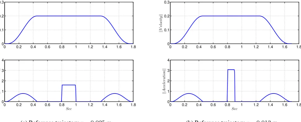
(a) Reference trajectoryr= 0.025m
0 0.2 0.4 0.6 0.8 1 1.2 1.4 1.6 1.8 0
0.1 0.2 0.3
||
V
el
oc
it
y
||
0 0.2 0.4 0.6 0.8 1 1.2 1.4 1.6 1.8 0
1 2 3 4
Sec
||
A
cc
el
er
a
ti
on
||
(b) Reference trajectoryr= 0.013m
Fig. 3: The norm of the velocity (in m/s) and the acceleration (in m/s
2) of reference trajectories.
motion of the portable mass remains constant as well as its
improving effect on the torque.
Figure 4b presents the result of the optimised torques
against non-optimised ones for the trajectory with a smaller
rounded corner radius (
i.e.
,
r
= 0
.
013
m). As can be seen in
the torque plot of joints
2
and
3
, the optimised value of the
torques are greater than the non-optimised value when the
end effector goes through the rounded corner. This is due to
the acceleration of the portable mass (
i.e.
,
s
¨
1) which meets
the pre-defined threshold (see Figure 6b). At this point, the
accelerations of the portable masses remain constant as well
as their effect on the inertial force of the distal link. Similar
to the results for the trajectory with
r
= 0
.
025
m, the velocity
of the portable mass two meets the limit at
t
= 0
.
4
s and the
corresponding acceleration drops to zero. It has been noticed
that the optimised value of the torque of joint
2
and
3
will
be less than non-optimised one if the limit of the
accelera-tion of the portable mass is increased to
12
m/s
2. Also, there
is a small jump at the optimised torque value of joint
1
at
t
= 0
.
8
s. This is due to the acceleration of the portable mass
that meets the limit.
Figure 5a shows the result of optimisation of the torques
for the trajectory with
r
= 0
.
025
m wile
λ
= 0
.
5
.
Since
the optimised torque values need to be as small as half of
the torque values of non-redundant manipulator, the portable
masses need to produce smaller inertial forces and moments
in comparison with the scenario with
λ
= 0
(Figure 4a.
Con-sequently, the portable masses move with smaller velocity
and acceleration (Figure 6c) which prevents them from
meet-ing the limits. As it is seen in Figure 6c, all portable masses
move with relatively smaller acceleration in comparison with
Figure 6a. Also, the second portable mass does not meet the
velocity limit at
t
= 0
.
65
s. The displacement of the portable
masses is shown in Figure 5b where they are initial at
0
and
The torque values of the joints are relatively small in all
cases when the end effector moves with a constant velocity.
When the acceleration of the end effector is zero, the inertial
forces and moments of the links decrease. In addition to that,
the inertial force of the end effector will turn to zero.
7
Conclusions
The dynamic model of a 3-RRR planar parallel manipulator
involving a portable mass on the distal links is developed.
The total of the squared actuators torques is investigated. An
optimisation algorithm is implemented to find the optimal
position of the portable masses while the end effector
under-goes an arbitrary trajectory with a rounded corner.
The concept was tested on two trajectories with different
rounded corners using the same Cartesian velocity. The
re-sults of the conducted tests suggest that the motion of the
portable masses can improve (
i.e.
, reduce) the ground
actu-ator torques for both accelerating and decelerating sections.
Also, the base actuator torques improve when the end
ef-fector tracks the rounded corner with
r
= 0
.
025
m.
How-ever, the optimised torques are greater than the the
non-optimised ones around the rounded corner for the trajectory
with
r
= 0
.
013
m. Since the trajectory with sharper corner
imposes greater torque values on the ground joints, the
mo-tion of the portable masses need to generate greater inertial
forces and moments on the distal links to improve the torque
values at rounded corner. However, the changes in inertial
forces and moments of the distal links are limited due the
limits that have been defined for the velocity and
accelera-tion of the portable masses.
The objective function is flexible to determine the
percent-age of improvement of the optimised torques with respect to
Figure 3.The norm of the velocity (in m s−1) and the acceleration (in m s−2) of reference trajectories.
as the difference between their objective function values are monitored at every iteration of optimisation. Once they have met the pre-defined user threshold, the opti-misation procedure stops.
7. Optimise the position of the portable mass: a non-linear multi-variable constrained optimisation is con-ducted to minimise the active-joint torques in Eq. (38).
– The displacement, velocity and acceleration of the
base actuators are calculated at every step of the optimisation procedure.
– The current velocity and acceleration of the
redun-dant actuators are calculated using the time history of the redundant actuators.
– The objective function value is determined.
5 Numerical example
5.1 Architectural parameters and analysed trajectory The manipulator’s architectural parameters for the current example are as follows: all proximal link lengths are set to 1 m (i.e., l1=1 m for all legs). Also, all distal link lengths are set to 1 m (i.e., l2=1 m for all legs) where a track has been attached to every distal link to allow the portable mass to move from si=−1 to 1 m. The base and moving platforms are equilateral triangles inscribed in circles of 1 m and 0.25 m in radius, respectively. The mass m1of each of the proximal links is 1 kg while the distal links have a mass m2=1 kg (in-cluding the mass of the track) and the end effector has mass
me=0.5 kg and ms=3 kg.
5.2 Trajectory planning
The procedure has been studied on two trajectories with rounded corners which have been planned in the Cartesian space. For both trajectories, the end effector moves on a straight line with an initial velocity of 0 m s−1while keeping the end effector with constant orientation. As the tracking velocity reaches a user defined velocity in a specified time (0.2 m s−1in 0.4 s), the end effector tracks the trajectory with a constant velocity. The abrupt acceleration change between
t=0.8 and t=1.0 s occurs when the end-effector enters the rounded corner segment and normal acceleration occurs. The end effector decelerates in (0.4 s) to come to a stop in the last point of the trajectory. However, the radii of the rounded cor-ners of the trajectories are different.
The trajectory’s initial position is p1=[1 0.4]T. Also, the radii of the round corners are r=0.025 m and r=0.013 m. Each trajectory starts from point p1 and goes in the positive
Y direction. Once the end effector moves 0.07 m in the Y di-rection, the rounded corner commences (the rounded corner is a quarter of a circle). Thereafter, the end effector travels 0.07 m in the negative x direction. The norm of the Cartesian velocity and the acceleration of the end effector is presented in Fig. 3. Since the radii of the rounded corners are different, the total length of the trajectories are not the same.
The optimisation problem was implemented in Matlab. The function fmincon was used to perform the constrained local optimisation in Eqs. (38) to (40). More particularly, the Sequential Quadratic Programming (SQP) with Hessian up-date option within fmincon was used. The SQP method is an alternative approach for handling inequality constraints in non-linear programming where SQP finds the minimum of a sequence of quadratic programming sub-problems. The ob-jective function is estimated with a quadratic function and
S. S. Parsa et al.: Internal redundancy to improve dynamic parameters in corners 239
8
S. S. Parsa, J. A. Carretero and R. Boudreau: Internal Redundancy to Improve Dynamic Parameters in Corners
0 0.2 0.4 0.6 0.8 1 1.2 1.4 1.6 1.8 −5
0 5
τ1
0 0.2 0.4 0.6 0.8 1 1.2 1.4 1.6 1.8 −5
0 5
τ2
0 0.2 0.4 0.6 0.8 1 1.2 1.4 1.6 1.8 −5
0 5
τ3
Sec
Optimized
No internal redundancy
(a) Base joint torque forr= 0.025m
0 0.2 0.4 0.6 0.8 1 1.2 1.4 1.6 1.8 −10
0 10
τ1
0 0.2 0.4 0.6 0.8 1 1.2 1.4 1.6 1.8 −10
0 10
τ2
0 0.2 0.4 0.6 0.8 1 1.2 1.4 1.6 1.8 −10
0 10
τ3
Sec
Optimized
No internal redundancy
(b) Base joint torque forr= 0.013m
Fig. 4:
The torques of the ground actuators (in N.m) forλ= 0.0 0.2 0.4 0.6 0.8 1 1.2 1.4 1.6 1.8 −5
0 5
τ1
0 0.2 0.4 0.6 0.8 1 1.2 1.4 1.6 1.8 −5
0 5
τ2
0 0.2 0.4 0.6 0.8 1 1.2 1.4 1.6 1.8 −5
0 5
τ3
Sec
Optimized
No internal redundancy
(a) Base joint torque
0 0.2 0.4 0.6 0.8 1 1.2 1.4 1.6 1.8 −1
0 1
S1
0 0.2 0.4 0.6 0.8 1 1.2 1.4 1.6 1.8 −1
0 1
S2
0 0.2 0.4 0.6 0.8 1 1.2 1.4 1.6 1.8 −1
0 1
Sec
S3
(b) Displacement of portable masses
Fig. 5:
The torques of the ground actuators (in N.m) and displacement of the portable masses (in m) forr= 0.025m andλ= 0.5.redundancy. As greater improvement of the torques requires
higher limits of the velocity and the acceleration for portable
masses, the objective function can be adjusted to keep the
optimisation variables away from the limits.
The obtained simulation results suggest that if a
manipu-lator can not follow a trajectory with a rounded corner due
to the torque limits of the ground joints, it will be
feasi-ble through application of internal redundancy (without
al-tering the ground actuators). This is possible as the dynamic
forces required to perform the more demanding trajectories
are shared by both the base actuators as well as the additional
actuators on the distal links.
There are a few parameters that affect the the simulation
such as Cartesian velocity of the end effector, the radius of
the rounded corner and the allowed limits of the velocity
ing a relatively large end effector velocity demands greater
torque values at the ground joints. Consequently, the portable
masses need to generate greater forces and moments on the
distal links which is proportional to the limits of the
veloc-ity and acceleration of the portable masses. Moreover, due
the aforementioned force sharing effect, the balance between
the contribution of the two sets of actuators to the specific
task needs to be carefully considered (
e.g.
, using an
objec-tive function that considers both sets of actuators).
As future work, it is suggested to look at the trajectory
globally rather than point-to-point motion planning. In that
case, the position of the portable masses can be adjusted with
respect to the any up-coming critical situation (
i.e.
, rounded
corner).
Figure 4.The torques of the ground actuators (in Nm) forλ=0.
is minimised subject to the linearised constraints. In this method, the Hessian of the Lagrangian function is estimated at every iteration using a quasi-Newton update method. This approximation is used to create a quadratic programming sub-problem and its solution is applied to generate a search direction for the line search procedure (Fletcher, 1987).
In the current numerical example, the velocity of the portable masses is allowed to vary in the range between −1 m s−1and+1 m s−1. The maximum absolute value of the acceleration of the portable masses is considered as 7 m s−2 and msi=3 kg for i=1,2,3.
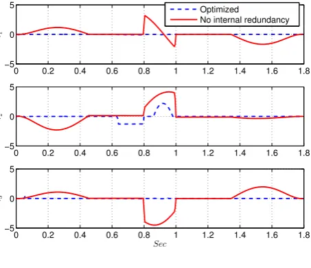
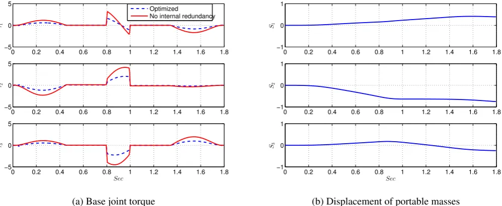
6 Results and discussion
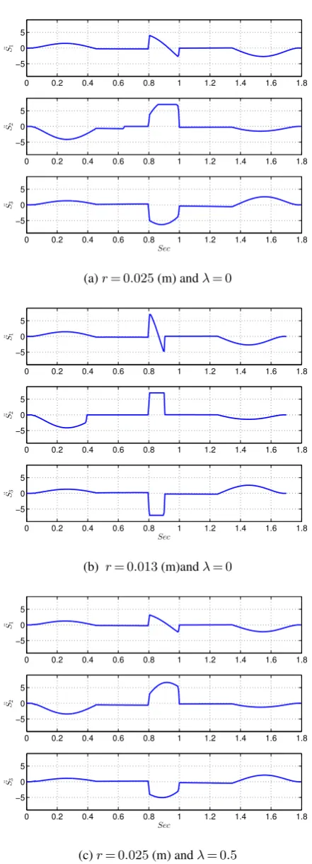
Figure 4a illustrates the comparison between the torque val-ues obtained from the optimisation routine and the manip-ulator without internal redundancy (i.e., msi=IBiA0i=0) for the trajectory with r=0.025 m as the radius of the rounded corner and λ=0. As shown in Fig. 4a, the manipulator with internal redundancy can follow the reference trajectory with significantly lower torques (approximately 10−1Nm) in both the accelerating and decelerating phases as well as the rounded corner area. However, the optimised torque for joint two is greater than the non-optimised one at t=0.65 s. As can be seen in Fig. 6a, the acceleration of the portable mass is zero at t=0.65 s which means the velocity of the portable mass meets the limits. Consequently, the effect of ¨s1is elim-inated from the dynamic equation at that instant. Also, the optimised torque for joint two at t=0.9 s is slightly greater than the optimised torque of actuators one and three at the same time instant. As it is shown in Fig. 6a, the accelera-tion of the second portable mass meets the limit at t=0.9 s. Consequently, the inertial force that is produced due to the
motion of the portable mass remains constant as well as its improving effect on the torque.
Figure 4b presents the result of the optimised torques against non-optimised ones for the trajectory with a smaller rounded corner radius (i.e., r=0.013 m). As can be seen in the torque plot of joints 2 and 3, the optimised value of the torques are greater than the non-optimised value when the end effector goes through the rounded corner. This is due to the acceleration of the portable mass (i.e., ¨s1) which meets the pre-defined threshold (see Fig. 6b). At this point, the ac-celerations of the portable masses remain constant as well as their effect on the inertial force of the distal link. Similar to the results for the trajectory with r=0.025 m, the velocity of the portable mass two meets the limit at t=0.4 s and the corresponding acceleration drops to zero. It has been noticed that the optimised value of the torque of joint 2 and 3 will be less than non-optimised one if the limit of the accelera-tion of the portable mass is increased to 12 m s−2. Also, there is a small jump at the optimised torque value of joint 1 at
t=0.8 s. This is due to the acceleration of the portable mass that meets the limit.
Figure 5a shows the result of optimisation of the torques for the trajectory with r=0.025 m wileλ=0.5. Since the op-timised torque values need to be as small as half of the torque values of non-redundant manipulator, the portable masses need to produce smaller inertial forces and moments in com-parison with the scenario withλ=0 (Fig. 4a). Consequently, the portable masses move with smaller velocity and acceler-ation (Fig. 6c) which prevents them from meeting the limits. As it is seen in Fig. 6c, all portable masses move with rela-tively smaller acceleration in comparison with Fig. 6a. Also, the second portable mass does not meet the velocity limit at
t=0.65 s. The displacement of the portable masses is shown
240 S. S. Parsa et al.: Internal redundancy to improve dynamic parameters in corners
8
S. S. Parsa, J. A. Carretero and R. Boudreau: Internal Redundancy to Improve Dynamic Parameters in Corners
0 0.2 0.4 0.6 0.8 1 1.2 1.4 1.6 1.8 −5
0 5
τ1
0 0.2 0.4 0.6 0.8 1 1.2 1.4 1.6 1.8 −5
0 5
τ2
0 0.2 0.4 0.6 0.8 1 1.2 1.4 1.6 1.8 −5
0 5
τ3
Sec
Optimized
No internal redundancy
(a) Base joint torque forr= 0.025m
0 0.2 0.4 0.6 0.8 1 1.2 1.4 1.6 1.8 −10
0 10
τ1
0 0.2 0.4 0.6 0.8 1 1.2 1.4 1.6 1.8 −10
0 10
τ2
0 0.2 0.4 0.6 0.8 1 1.2 1.4 1.6 1.8 −10
0 10
τ3
Sec
Optimized
No internal redundancy
(b) Base joint torque forr= 0.013m
Fig. 4:
The torques of the ground actuators (in N.m) forλ= 0.0 0.2 0.4 0.6 0.8 1 1.2 1.4 1.6 1.8 −5
0 5
τ1
0 0.2 0.4 0.6 0.8 1 1.2 1.4 1.6 1.8 −5
0 5
τ2
0 0.2 0.4 0.6 0.8 1 1.2 1.4 1.6 1.8 −5
0 5
τ3
Sec
Optimized
No internal redundancy
(a) Base joint torque
0 0.2 0.4 0.6 0.8 1 1.2 1.4 1.6 1.8 −1
0 1
S1
0 0.2 0.4 0.6 0.8 1 1.2 1.4 1.6 1.8 −1
0 1
S2
0 0.2 0.4 0.6 0.8 1 1.2 1.4 1.6 1.8 −1
0 1
Sec
S3
(b) Displacement of portable masses
Fig. 5:
The torques of the ground actuators (in N.m) and displacement of the portable masses (in m) forr= 0.025m andλ= 0.5.redundancy. As greater improvement of the torques requires
higher limits of the velocity and the acceleration for portable
masses, the objective function can be adjusted to keep the
optimisation variables away from the limits.
The obtained simulation results suggest that if a
manipu-lator can not follow a trajectory with a rounded corner due
to the torque limits of the ground joints, it will be
feasi-ble through application of internal redundancy (without
al-tering the ground actuators). This is possible as the dynamic
forces required to perform the more demanding trajectories
are shared by both the base actuators as well as the additional
actuators on the distal links.
There are a few parameters that affect the the simulation
such as Cartesian velocity of the end effector, the radius of
the rounded corner and the allowed limits of the velocity
and acceleration of the portable masses. For instance,
hav-ing a relatively large end effector velocity demands greater
torque values at the ground joints. Consequently, the portable
masses need to generate greater forces and moments on the
distal links which is proportional to the limits of the
veloc-ity and acceleration of the portable masses. Moreover, due
the aforementioned force sharing effect, the balance between
the contribution of the two sets of actuators to the specific
task needs to be carefully considered (
e.g.
, using an
objec-tive function that considers both sets of actuators).
As future work, it is suggested to look at the trajectory
globally rather than point-to-point motion planning. In that
case, the position of the portable masses can be adjusted with
respect to the any up-coming critical situation (
i.e.
, rounded
corner).
Acknowledgement. The authors acknowledge the financial support
Figure 5.The torques of the ground actuators (in Nm) and displacement of the portable masses (in m) for r=0.025 m andλ=0.5.
in Fig. 5b where they are initial at 0 and are allowed to move between−1 and 1.
The torque values of the joints are relatively small in all cases when the end effector moves with a constant velocity. When the acceleration of the end effector is zero, the inertial forces and moments of the links decrease. In addition to that, the inertial force of the end effector will turn to zero.
7 Conclusions
The dynamic model of a 3-RRR planar parallel manipulator involving a portable mass on the distal links is developed. The total of the squared actuators torques is investigated. An optimisation algorithm is implemented to find the optimal position of the portable masses while the end effector under-goes an arbitrary trajectory with a rounded corner.
The concept was tested on two trajectories with different rounded corners using the same Cartesian velocity. The re-sults of the conducted tests suggest that the motion of the portable masses can improve (i.e., reduce) the ground ac-tuator torques for both accelerating and decelerating sec-tions. Also, the base actuator torques improve when the end effector tracks the rounded corner with r=0.025 m. How-ever, the optimised torques are greater than the the non-optimised ones around the rounded corner for the trajectory with r=0.013 m. Since the trajectory with sharper corner im-poses greater torque values on the ground joints, the motion of the portable masses need to generate greater inertial forces and moments on the distal links to improve the torque values at rounded corner. However, the changes in inertial forces and moments of the distal links are limited due the limits that have been defined for the velocity and acceleration of the portable masses.
The objective function is flexible to determine the percent-age of improvement of the optimised torques with respect to the torque values of the same manipulator without internal redundancy. As greater improvement of the torques requires higher limits of the velocity and the acceleration for portable masses, the objective function can be adjusted to keep the optimisation variables away from the limits.
The obtained simulation results suggest that if a manipu-lator can not follow a trajectory with a rounded corner due to the torque limits of the ground joints, it will be feasi-ble through application of internal redundancy (without al-tering the ground actuators). This is possible as the dynamic forces required to perform the more demanding trajectories are shared by both the base actuators as well as the additional actuators on the distal links.
There are a few parameters that affect the the simulation such as Cartesian velocity of the end effector, the radius of the rounded corner and the allowed limits of the velocity and acceleration of the portable masses. For instance, hav-ing a relatively large end effector velocity demands greater torque values at the ground joints. Consequently, the portable masses need to generate greater forces and moments on the distal links which is proportional to the limits of the veloc-ity and acceleration of the portable masses. Moreover, due the aforementioned force sharing effect, the balance between the contribution of the two sets of actuators to the specific task needs to be carefully considered (e.g., using an objec-tive function that considers both sets of actuators).
S. S. Parsa et al.: Internal redundancy to improve dynamic parameters in corners 241
S. S. Parsa, J. A. Carretero and R. Boudreau: Internal Redundancy to Improve Dynamic Parameters in Corners 9
0 0.2 0.4 0.6 0.8 1 1.2 1.4 1.6 1.8 −5
0 5 ¨S1
0 0.2 0.4 0.6 0.8 1 1.2 1.4 1.6 1.8 −5
0 5 ¨S2
0 0.2 0.4 0.6 0.8 1 1.2 1.4 1.6 1.8 −5
0 5
Sec
¨S3
(a)r= 0.025(m) andλ= 0
0 0.2 0.4 0.6 0.8 1 1.2 1.4 1.6 1.8 −5
0 5 ¨S1
0 0.2 0.4 0.6 0.8 1 1.2 1.4 1.6 1.8 −5
0 5 ¨S2
0 0.2 0.4 0.6 0.8 1 1.2 1.4 1.6 1.8 −5
0 5
Sec
¨S3
(b) r= 0.013(m)andλ= 0
0 0.2 0.4 0.6 0.8 1 1.2 1.4 1.6 1.8 −5
0 5 ¨S1
0 0.2 0.4 0.6 0.8 1 1.2 1.4 1.6 1.8 −5
0 5 ¨S2
0 0.2 0.4 0.6 0.8 1 1.2 1.4 1.6 1.8 −5
0 5
Sec
¨S3
(c)r= 0.025(m) andλ= 0.5
Fig. 6:The acceleration of the portable masses (in m/s2).
from the Natural Science and Engineering Research council of Canada through their Discovery Grant program.
References
Boudreau, R. and Nokleby, S.: Force Optimisation of kinematically-redundant planar parallel manipulators following a desired trajectory, Mechanism and Machine Theory, 56, 138– 155, 2012.
Cha, S., Lasky, T. A., and Velinsky, S. A.: Kinematically-Redundant Variations of the 3-RRR Mechanism and Local Optimization-Based Singularity Avoidance, Mechanism Based Design of Structures and Machines, 35, 15–38, 2007.
Cheng, H., Yiu, Y.-K., and Li., Z.: Dynamics and Control of Redun-dantly Actuated Parallel Manipulators, IEEE/ASME Transac-tions on Mechatronics, 8, 483–491, doi:10.1109/TMECH.2003. 820006, 2003.
Cheng, H., Liu, G. F., Yiu, Y. K., Xiong, Z. H., and Li, Z.: Ad-vantages and dynamics of parallel manipulators with redundant actuation, in: Proceedings of the IEEE/RSJ International Con-ference on Intelligent Robots and Systems, pp. 171–176, Maui, USA, 2011.
Ebrahimi, I., Carretero, J. A., and Boudreau, R.: Kinematic anal-ysis and path planning of a new kinematically redundant planar parallel manipulator, Robotica, 26, 405–413, 2008.
Firmani, F. and Podhorodeski, R. P.: Force-unconstrained poses for a redundantly actuated planar parallel manipulator, Mechanism and Machine Theory, 39, 459–476, 2004.
Firmani, F., Zibil, A., Nokleby, S. B., and Podhorodeski, R. P.: Force-Moment Capabilities of Revolute-Jointed Planar Parallel Manipulators with Additional Actuated Branches, Transactions of the Canadian Society for Mechanical Engineering, 31, 469– 481, http://www.tcsme.org/Vol31-No4.html, 2007.
Fletcher, R.: Practical Methods of Optimization, John Wiley and Sons, 1987.
Garg, V., Carretero, J. A., and Nokleby, S. B.: A New Method to Determine the Force and Moment Workspaces of Actuation Re-dundant Spatial Parallel Manipulators, Journal of Mechanisms and Robotics, 1, 1–8, doi:10.1115/1.3147184, 2009.
Gosselin, C. and Angeles, J.: The optimum kinematic design of a planar three-degree-of-freedom parallel manipulator, Journal of Mechanism, Transmissions, and Automation in Design, 110, 35– 41, 1988.
Lee, S. and Kim, S.: Kinematic analysis of generalized parallel ma-nipulator systems., in: Proceedings of the IEEE Conference on Decision and Control, vol. 2, pp. 1097–1102, 1993.
Merlet, J.-P.: Redundant parallel manipulators, Laboratory Robotics and Automation, 8, 17–24, 1996.
Nokleby, S. B., Fisher, R., Podhorodeski, R. P., and Firmani, F.: Wrench capabilities of redundantly-actuated parallel manip-ulators, Mechanism and Machine Theory, 40, 578–599, doi: 10.1016/j.mechmachtheory.2004.10.005, 2005.
Ruggiu, M. and Carretero, J. A.: Kinematic Analysis of the 3-PRPR Redundant Planar Parallel Manipulator, in: Proceedings of the 2009 CCToMM Symposium on Mechanisms, Machines, and Mechatronics, Qu´ebec, Canada, 2009.
Ruggiu, M. and Carretero, J. A.: Actuation strategy based on the acceleration model for the 3-PRPR redundant planar parallel ma-nipulator, in: Advances in Robot Kinematics: Analysis and
De-Figure 6.The acceleration of the portable masses (in m s−2).
Acknowledgement. The authors acknowledge the financial
support from the Natural Science and Engineering Research council of Canada through their Discovery Grant program.
Edited by: A. M¨uller
Reviewed by: two anonymous referees
References
Boudreau, R. and Nokleby, S.: Force Optimisation of kinematically-redundant planar parallel manipulators following a desired tra-jectory, Mech. Mach. Theory, 56, 138–155, 2012.
Cha, S., Lasky, T. A., and Velinsky, S. A.: Kinematically-Redundant Variations of the 3-RRR Mechanism and Local Optimization-Based Singularity Avoidance, Mechanism Optimization-Based Design of Structures and Machines, 35, 15–38, 2007.
Cheng, H., Yiu, Y.-K., and Li, Z.: Dynamics and Con-trol of Redundantly Actuated Parallel Manipulators, IEEE/ASME Transactions on Mechatronics, 8, 483–491, doi:10.1109/TMECH.2003.820006, 2003.
Cheng, H., Liu, G. F., Yiu, Y. K., Xiong, Z. H., and Li, Z.: Ad-vantages and dynamics of parallel manipulators with redundant actuation, in: Proceedings of the IEEE/RSJ International Confer-ence on Intelligent Robots and Systems, 171–176, Maui, USA, 2011.
Ebrahimi, I., Carretero, J. A., and Boudreau, R.: Kinematic analy-sis and path planning of a new kinematically redundant planar parallel manipulator, Robotica, 26, 405–413, 2008.
Firmani, F. and Podhorodeski, R. P.: Force-unconstrained poses for a redundantly actuated planar parallel manipulator, Mech. Mach. Theory, 39, 459–476, 2004.
Firmani, F., Zibil, A., Nokleby, S. B., and Podhorodeski, R. P.: Force-Moment Capabilities of Revolute-Jointed Planar Parallel Manipulators with Additional Actuated Branches, T. Can. Soc. Mech. Eng., 31, 469–481, http://www.tcsme.org/Vol31-No4. html, 2007.
Fletcher, R.: Practical Methods of Optimization, John Wiley and Sons, 1987.
Garg, V., Carretero, J. A., and Nokleby, S. B.: A New Method to Determine the Force and Moment Workspaces of Actuation Re-dundant Spatial Parallel Manipulators, Journal of Mechanisms and Robotics, 1, 1–8, doi:10.1115/1.3147184, 2009.
Gosselin, C. and Angeles, J.: The optimum kinematic design of a planar three-degree-of-freedom parallel manipulator, Journal of Mechanism, Transmissions, and Automation in Design, 110, 35– 41, 1988.
Lee, S. and Kim, S.: Kinematic analysis of generalized parallel ma-nipulator systems, in: Proceedings of the IEEE Conference on Decision and Control, 2, 1097–1102, 1993.
Merlet, J.-P.: Redundant parallel manipulators, Lab. Robotics Au-tomat., 8, 17–24, 1996.
Nokleby, S. B., Fisher, R., Podhorodeski, R. P., and Fir-mani, F.: Wrench capabilities of redundantly-actuated parallel manipulators, Mech. Mach. Theory, 40, 578–599, doi:10.1016/j.mechmachtheory.2004.10.005, 2005.
242 S. S. Parsa et al.: Internal redundancy to improve dynamic parameters in corners
Ruggiu, M. and Carretero, J. A.: Actuation strategy based on the acceleration model for the 3-PRPR redundant planar parallel ma-nipulator, in: Advances in Robot Kinematics: Analysis and De-sign, edited by: Lenarˇciˇc, J. and Stanisic, M. M., Springer, Piran-Portoroˇz, Slovenia, 2010.
Vukobratovi´c, M., Potkonjak, V., and Matijevi´c, V.: Internal redun-dancy – the way to improve robot dynamics and control perfor-mances, J. Intell. Robot. Syst., 27, 31–66, 2000.
Wang, J. and Gosselin, C. M.: Kinematic Analysis and Design Of Kinematically Redundant Parallel Mechanisms, J. Mech. Design, 126, 109–118, 2004.
Wu, J., Wang, J., Wang, L., and Tiemin, L.: Dynamics and control of a planar 3-DOF parallel manipulator with actuation redundancy, Mech. Mach. Theory, 44, 835–849, 2009.
Wu, J., Wang, J., and You, Z.: A comparison study on the dynamics of planar 3-DOF 4-RRR, 3-RRR and 2-RRR parallel manipula-tors, Journal of Robotics and Computer Integrated Manufactur-ing, 27, 150–156, 2011.