Assessing the Future of Renewable and Smart Grid Technologies in Regional Energy Systems

(1)

a This research has been supported by the GICC programme of the French Ministry MEDDEM, by the EUFP7-ERMITAGE research project, by the project RITES, financed by the Federal Office for Energy, Bern, Switzerland and by the Swiss-NSF-NCCR climate grant.

b ORDECSYS, Switzerland and Economics and Environmental Management Laboratory – Swiss Federal Institute of Technology at Lausanne (EPFL), Switzerland.

c ORDECSYS, 4 Place de l’Etrier Chêne Bougeries, 1224 Switzerland. www.ordecsys.com. d Economics and Environmental Management Laboratory – Swiss Federal Institute of

Technol-ogy at Lausanne (EPFL), Switzerland. e ORDECSYS, Switzerland.

Technologies in Regional Energy Systems

F. Babonneaub_{, A. Haurie}c_{, G. J. Tarel}d_{and J. Thénié}e

JEL-Classification: Q41,Q42

Keywords: smart-grids, renewable energy sources, Switzerland, Geneva

1. Introduction

(2)

(Galus and Andersson, 2008; Marnay et al., 2008). The electricity produc-tion system will evolve toward more decentralizaproduc-tion, with two-way communi-cation channels permitting the coordination and optimization of the actions of myriad of agents involved in local consumption and production. This intelligent distribution system will also improve the system services like, e.g., peak-load or demand management (Shin-ichi, 2010).

The assessment of the future role of these renewable technologies in associa-tion with smart grid technologies can be made at a regional level, correspond-ing to the size of a local distribution grid. In Switzerland this corresponds to a cantonal or sub-cantonal level. In this paper we propose to represent smart grid technologies as well as intermittent electricity production into the energy-tech-nology-environment model ETEM that is adapted for modeling energy sys-tems at a regional level. The resulting model is applied to a case study, roughly calibrated on the Geneva cantonal data, to assess the future of renewable and smart grid technologies. To take into account some of the uncertainties on smart grids development, we complement our study with stochastic considerations on availability of green electricity imports (contingent, e.g., to the development of DESERTEC) and electric car technologies.

(3)

1 For more information, see the reference manual (Drouet and Thénié, 2009) available on the web site www.ordecsys.com.

2 Please visit the web site www.ordecsys.com.

2. ETEM

2.1 A Member of the MARKAL-TIMES Family of Models

ETEM, for Energy-Technology-Environment Model1_{, is a regional bottom-up} model that has been designed for modeling energy systems at a regional level. ETEM is a bottom-up model that gives a representation of the energy and tech-nology choices that could best deliver the needed energy services in a given region. The ETEM model rationale is to supply energy services at minimum global cost, over a planning horizon, typically of 45–50 years, permitting one to envision major changes in the technology portfolio. The total discounted cost, which is the objective function to be minimized, includes investment, operat-ing cost and energy imports and exports. A salvage value takes into account the end-of-planning horizon valuation of the remaining technology capacities. The regional scope of ETEM makes it particularly well-suited to model and analyze renewable and smart grid technologies, which are necessarily connected to a regional distribution grid.

(4)

for an energy system corresponding to the Geneva canton. A version of ETEM for Luxembourg has been developed and a coupling with an air pollution model has been realized (Zachary et al., 2011). Another open-source energy model, OSeMOSYS, similar to MARKAL and also programmed in GMPL has been recently announced by a group of prominent energy modelers (see Howells et al., 2011); the originality in this model is essentially the possibility to run it with free access open-source software, thus reducing the upfront cost of a modeling exercise. The introduction of the open-source model OSeMOSYS confirms the value of the options taken when developing ETEM.

An ETEM model has the following attractive features:

– flexible representation of an energy system, exploiting geographical data; – fast techno-economic database building through a new web based interface; – linkage ability with macro-economic or environmental simulation models; – modularity and capacity to accept easily new features, like new equations to

describe constraints at a local level, transmission and grid related constraints, nonlinear optimization, stochastic optimization, etc.

2.2 The Reference Energy System

ETEM is driven by projections of useful (energy services) demands, for differ-ent economic sectors, over a time horizon ranging between 25 and 100 years. These projections are determined by a set of drivers concerning, e.g., the demo-graphic or GDP growth.

(5)

Fi

g

u

re 1

: A Si

mple R ef er enc e E n er g y S ys te m El ec tri ci ty (p ower pl an t) He at (t ra n sf er fl u id ) O il p rod u ct io n s, Sy n th et ic f u el s, Biof u el s, Bio ga s R esi den ti al S upply Dem an d Pr im ar y en erg y R ene w ab le Rec ycl ed wa st e Biom as s Im po rt at io ns Ex p ort at io n s Sm ar t G rid T ec h nolo gi es pr o du ct ion /c onve rs ion /s tor ag e/ end u se L ig ht E le c. A ppl ia nc e He at in g E le c. A ppl ia nc e P u bl ic / Pr iv at e / Tr u ck Co mm er ci al Pub li c In d u st ria l Tr an sp or t L ig

ht / He

at

in

g / W

ar

m

w

at

er / E

le c. A p p li an ce He at in

g / C

(6)

The main difference between a national or multi-national model, like TIMES, and a regional model like ETEM is in the emphasis given in the latter to the rep-resentation of demand technologies for residential and commercial heat, sanitary water, transportation (public and private) and captive electricity usages, whereas energy uses in industry, refineries and nuclear plants are not considered in full details. ETEM contains a detailed description of the distribution of electricity, natural gas and heat through networks. It can also give an accurate represen-tation of the potential of renewable energy for decentralized electricity or heat production.

A few more details concerning the main equations of the model are given in the Annex. It suffices to say, for the moment, that ETEM is a linear programming model. It is very efficient for the description of economic activities that satisfy the diminishing marginal return paradigm, which corresponds to the use of convex cost functions or concave production functions. It permits also the modeling of increasing marginal returns, or concave cost function, through the introduction of mixed-integer programming optimization techniques.

3. Representation of Smart Grid Technologies

Smart grids allow smart energy management through the use of technologies with two-way communication abilities that are acting as consumption, storage or production units, depending on the location and time-slice of the load curve. The temporary electricity storage activity is currently performed by hydroelec-tric pumped-storage facilities. The announced penetration of elechydroelec-tric or plug-in hybrid electric cars and of small gas fuel-cell with heat storage etc. will permit a further extension of the temporary storage activity provided a smart-grid environ-ment exists. We describe below how we have represented in the model some of the demand technologies, for transport, residential and commercial heating and for renewable electricity production that can be linked together through a smart grid.

3.1 Representation of Temporary Storage

(7)

rep-We need to distinguish the demand technology from its storage capacity, when this capacity exists. So we create a commodity of storage between the demand technology and its storage unit. For example, the technology electric car is decom-posed between the technology car and the technology battery. We distinguish the commodities electricity, electricity for storage, electricity for transport and represent their flows at different time-slices. We can then represent the use of batteries to provide the transportation service and also to contribute to the electricity system service, in particular to satisfy peak load demand. We show below how this tech-nology is represented in the RES.

3.2 Electric Vehicle

We assume in this study that electric vehicles with their batteries can contrib-ute to peak load reserve requirements in all time-slices; they also allow storage of electricity produced during low demand time-slice and to be used during the time-slice of highest demand. The techno-economic parameters of the electric vehicle have been defined in accordance with Kempton and Tomić, 2005. To model electric vehicle in ETEM, we adopt the approach illustrated in Figure 2. As indicated before, we decompose the electric vehicle technology into two sepa-rated technologies, i.e., vehicle and battery, with the constraint that the number of batteries is lower than three times the number of vehicles (some variations on this constraint will be discussed later). The input of both technologies is elec-tricity while the outputs are different: vehicles produce a service of car tranport (measured in 1000 kilometer q vehicles per day) while batteries give an energy form: electricity (in PJ). The technology battery has a positive contribution to peak-load reserve constraints.

(8)

during the day for a release to the electric grid. In forthcoming implementations other options will be explored, for instance the option where an empty battery is replaced by a recharged one at a service station containing a lot of batteries that could also be used for temporary storage.

3.3 Photovoltaic Units

The representation of photovoltaic (PV) units is given in Figure 3. We assume here that all produced electricity is used directly for demand satisfaction and so PV units are not connected to storage technologies. The intermittent produc-tion is considered, with an availability of 10% in winter-day, 40% in summer-day and 20% in intermediate-summer-day while the availability of PV units is fixed at 0 during night time-slices. The life time of a PV is fixed at 30 years, and 25% of the capacity can contribute to the peak of consumption during the day. The cost of PV panels corresponds to a price of 0.17 CHF/kWh.

3.4 Wind Mills

The representation of winds mills is given in Figure 4. The overall energy con-version efficiency is taken as 40%. The intermittent production is considered, with an availability of 30% over a year. The life time of a wind mill is fixed at 25 years. The electricity produced by wind mills has a cost of 0.025 CHF/kWh.

Figure 2: Electric Vehicle Modeling in ETEM

Electricity for transport Electricity for storage Transport

Electric car

(9)

3.5 Decentralized Combined Heat Power Production

Among the new technologies that could link residential or commercial heat-ing systems with smart grids, we have retained the small gas powered fuel cell combined heat power (CHP) with temporary storage of heat. These decentral-ized units (like e.g. those based on SOFC fuell-cells) can produce electricity during time-slices of high demand and store the heat for use during the rest of the day. They are considered as promising contributors to a rationalization of

Figure 3: Modeling of PV Units in ETEM

Solar Electricity for storage Electricity

solar plant

Figure 4: Modeling of Wind Mills in ETEM

Wind Electricity for storage Electricity

(10)

both electric and gas grids (Acha, Green, and Shah, 2010b; Streckiene et al., 2009). Within ETEM, the cost of such production unit is taken as 1,000 Mil-lions of CHF per GW starting from 2015, with a maximum of 35% of electric-ity (and a minimum of 65% of heat). We base our cost evaluation on Huang, Zhang, and Jiang (2006), Brown, Hendry, and Harborne (2007), Neef (2009), and Hawkes and Leach (2007). We expect prices to drop by 2015 (see e.g. http://www1.eere.energy.gov/hydrogenandfuelcells/fuelcells/systems.html). As well, data coming from manufacturers when available (Panasonic, CERES power) and from large-scale tests in Japan are used.

Figure 5: CHP Modeling in ETEM

NGA Heat for storage Heat Electricity CO2

CHP

Heat storage

3.6 Geothermal Units

(11)

4 Other data, like technology specificities for instance, are mainly calibrated with ETSIAP, IEA and cantonal offices of statistics and energy.

Figure 6: Geothermal Units Modeling in ETEM

Electricity Heat

Geothermal units

This simple geothermal unit is a decentralized renewable technology, which will not benefit from a two-way communication system and will not contribute to the electricity system service.

4. Scenario Analysis

4.1 Application to Geneva

(12)

4.2 Useful Demand and Imported Energy Price Projections

4.2.1 Demands

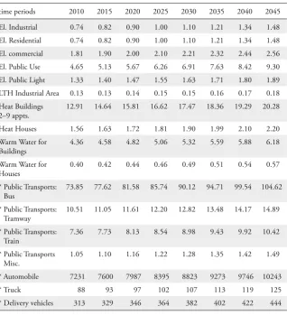
Table 1 summarizes the assumptions on useful demands. We assume the typi-cal building and housing replacement rate of 1% generally accepted in Euro-pean cities.

Table 1: Useful Demands (PJ/Y or * 1000 kmqVehicle/Day)

time periods 2010 2015 2020 2025 2030 2035 2040 2045 El. Industrial 0.74 0.82 0.90 1.00 1.10 1.21 1.34 1.48 El. Residential 0.74 0.82 0.90 1.00 1.10 1.21 1.34 1.48 El. commercial 1.81 1.90 2.00 2.10 2.21 2.32 2.44 2.56 El. Public Use 4.65 5.13 5.67 6.26 6.91 7.63 8.42 9.30 El. Public Light 1.33 1.40 1.47 1.55 1.63 1.71 1.80 1.89 LTH Industrial Area 0.13 0.13 0.14 0.15 0.15 0.16 0.17 0.18 Heat Buildings

2–9 appts.

12.91 14.64 15.81 16.62 17.47 18.36 19.29 20.28 Heat Houses 1.56 1.63 1.72 1.81 1.90 1.99 2.10 2.20 Warm Water for

Buildings

4.36 4.58 4.82 5.06 5.32 5.59 5.88 6.18 Warm Water for

Houses

0.40 0.42 0.44 0.46 0.49 0.51 0.54 0.57 * Public Transports:

Bus

Tramway

Train

7.36 7.73 8.13 8.54 8.98 9.43 9.92 10.42 * Public Transports

Misc.

1.05 1.10 1.16 1.22 1.28 1.35 1.42 1.49 * Automobile 7231 7600 7987 8395 8823 9273 9746 10243

* Truck 88 93 97 102 107 113 119 125

(13)

5 The demands are exogenous. The computation with drivers are made before modeling. 6 Using ETSAP-IEA data (http://www.iea-etsap.org/web/Demand.asp) and other sources. Except for transportation, we represent the demand for energy services by the amount of energy used during a year. The demands of transport are represented in 1000s vehicle q km per day.

In order to project the demand evolution5_{over the time horizon of 2045 we use} two drivers: (i) a GDP driver assumed to be growing at 2% per year (for indus-trial and commercial electricity and commercial heat); (ii) a demographic driver assumed to be growing at 1% per year (for remaining demands). The population of the region considered is 460,000 in 2010.

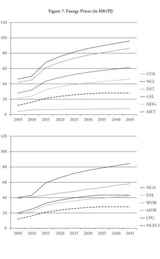
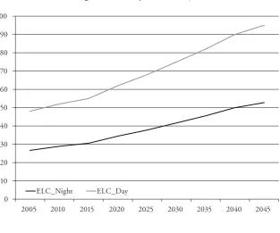
4.2.2 Energy Prices

The second set of important drivers of the model concerns the evolution of energy prices. For end-use prices in 2005 and 2010, we use IEA (2011a) valid for Swit-zerland including taxes. On top of that, we use projections for fossil fuels that are consistent with those proposed by IEA (2011b). Figures 7–8 summarize these assumptions. The prices are given in million-CHF per PJ (Mfr/PJ).

For electricity we distinguish two price levels, a high one during day time-slices (from 50 MCHF/PJ in 2010 to 95 MCHF/PJ in 2045) and a lower one during night time-slices (from 26 MCHF/PJ in 2010 to 52 MCHF/PJ in 2045). These price schedules include taxes and are consistent with those proposed in the com-panion paper (Weidmann, Kannan, and Turton, 2012, which analyses the electricity sector in Switzerland.

4.3 Residual Capacities and Calibration on Year 2010

4.3.1 Identification of Residual Capacities

(14)

Figure 7: Energy Prices (in Mfr/PJ)

0 20 40 60 80 100 120

2005 2010 2015 2020 2025 2030 2035 2040 2045

NGA NGI

WOR

MSW

LPG

NGFCC 0

20 40 60 80 100 120

2005 2010 2015 2020 2025 2030 2035 2040 2045

COA

DSL DST

GSL

HDG

(15)

Table 2: Residual Capacities: Heat and Warm Water (PJ/Y)

2010 2015 2020 2025 2030 2035 2040 2045 Existing houses

Oil furnace heat & warm water

0.0247 0.0212 0.0176 0.0141 0.0106 0.007 0.0035 0 Gas furnace heat

& warm water

0.0439 0.0376 0.0063 0.0051 0.0038 0.0025 0.0013 0

Existing buildings Oil furnace heat

& warm water

0.2191 0.1799 0.1481 0.1463 0.1145 0.0827 0.0508 0 Gas furnace heat

& warm water

0.2655 0.2424 0.2238 0.1853 0.1367 0.0981 0.0395 0 Gas furnace 0.0940 0.0686 0.0571 0.0457 0.0343 0.0229 0.0114 0

Figure 8: Electricity Prices (Mfr/PJ)

0 10 20 30 40 50 60 70 80 90 100

(16)

2010 2015 2020 2025 2030 2035 2040 2045 New buildings

Oil furnace heat & warm water

0.1389 0.118 0.0944 0.076 0.057 0.038 0.019 0.01

Warm Water Buildings

Elect. warm water 0.0334 0.025 0.022 0.015 0.013 0 0 0 Gas warm water 0.0334 0.025 0.022 0.015 0.013 0 0 0

Warm Water houses

Elect. warm water 0.0317 0.0273 0.0218 0.0175 0.0134 0.089 0.0445 0

Table 3: Residual Capacities: Transport (1000 kmqVehicle / Day)

2010 2015 2020 2025 2030 2035 2040 2045 Public Transport

Diesel Bus 66.23 26.6 10.7 4.3 1.8 0.7 0 0

Trolleybus 7.64 3.82 1.15 0.46 0 0 0 0

Tramway 15.2 8.9 5.3 3.1 0 0 0 0

Train 15.6 9.2 5.4 3.2 0 0 0 0

Miscellaneous 1.51 0.5 0 0 0 0 0 0

Private Transport

Diesel car 1228 600 186 74 0 0 0 0

Gasoline car 6003 3000 909 360 0 0 0 0

Trucks

Diesel truck 88.1 41.9 0 0 0 0 0 0

Delivery vehicles

Light diesel truck 63 31.09 0 0 0 0 0 0

Light gasoline truck 251 150.28 0 0 0 0 0 0

(17)

Table 4: Residual Capacities: Centralised Conversion Technologies (MW)

Type, Location 2010 2015 2020 2025 2030 2035 2040 2045

Hydro, Chancy-Pougny 44 44 44 53 53 53 53 53

Hydro, Seujet 5.5 5.5 5.5 5.5 5.5 5.5 5.5 5.5

Hydro, Vessy 0.25 0.25 0.25 0.25 0.25 0.25 0.25 0.25 Hydro, Project Conflan 0 0 0 0 25 25 25 25

Photovoltaic, Total 12 15 15 7 3 0 0 0

Wind, Total 1 56 56 56 56 56 0 0

Municipal waste CHP, Cheneviers

40 40 40 40 40 40 40 40

Hydro, Verbois 98 98 98 98 98 98 98 98

4.3.2 Calibration in 2010

From the residual capacities of current technologies and their technical coeffi-cients describing input and output of commodities, we can compute the share of different energy forms in the primary energy balance, the use of different energy forms by end-use sectors and the energy imports (see Figures 9–11). These fig-ures show that the model is correctly calibrated on the situation prevailing in the canton of Geneva in 2010.

Figure 9: Distribution of Primary Energy Forms for Geneva in 2010 (in%).

Coal 0%

Gas 40%

Hydroelectricity 17% Renewables

0% Oil 40%

(18)

Figure 10: Distribution of Energy Consumption by End-Use Sectors for Geneva in 2010 (in%).

Oil (heat) 26%

Gas 27% Oil (transport)

23% Electricity

22% District heating

2%

Figure 11: Distribution of Energy Imports for Geneva in 2010 (in%).

Electricity 18%

Fuel-Oil 17%

Gas 41% Unleaded

Gasoline 18% Diesel for transport

(19)

4.4 Assessing New Technology Impacts on Three Contrasted Scenarios

In this subsection, we compare the energy system evolutions of the Geneva canton on three contrasted scenarios and we highlight the role of renewable and smart-grid technologies in those evolutions.

4.4.1 CO₂ Emission Targets

The three scenarios differ by their CO₂ emission targets and the limit imposed on electricity imports. The BAU scenario has no limitation on GHG emissions and no restriction concerning electricity imports. The Factor-4 scenario aims at a reduction by 4 of the current emission levels (2 Mt CO₂). The objective is thus to decrease to 0.4 Mt CO₂ in 2045. The Regulation scenario aims at limiting the electricity imports at 15 PJ/Year (corresponding roughly to 50% of the electric-ity imports in scenario Factor-4) and reducing the GHG emissions to 1.25 Mt CO₂. These three targets are represented in Figure 12.

Figure 12: Emissions in Mt of CO2 Equivalent for the Three Contrasted Scenarios.

0 0.5 1 1.5 2 2.5 3

2005 2010 2015 2020 2025 2030 2035 2040 2045

(20)

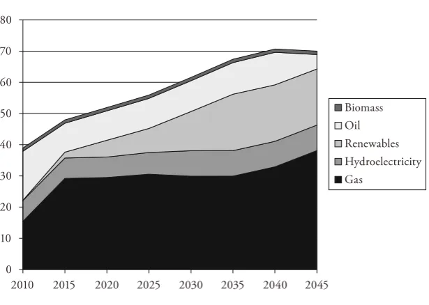
4.5 BAU Scenario

In the Business as usual (BAU) scenario, GHG emission reaches a value close to 2.7 MtC/Y of CO₂ in 2040. This is explained partly by the stable contribution of oil (to be used mainly in transport) and the strong penetration of gas in the primary energy balance, as shown in Figure 13.

Figure 13: Primary Energy (PJ/Year) – BAU Case.

0 10 20 30 40 50 60 70 80

2010 2015 2020 2025 2030 2035 2040 2045

Biomass Oil Renewables Hydroelectricity Gas

(21)

Table 5: Centralized Conversion Technologies (MW)

Type, Location 2010 2015 2020 2025 2030 2035 2040 2045

Hydro, Chancy-Pougny 44 44 44 53 53 53 53 53

Hydro, H. Project Seujet 5.5 5.5 5.5 5.5 5.5 5.5 5.5 5.5 Hydro, H. Vessy 0.25 0.25 0.25 0.25 0.25 0.25 0.25 0.25

Hydro, H. Conflan 0 0 0 0 25 25 25 25

Photovoltaic, Total 12 15 15 7 3 0 0 62

District heat, Total 25 16 16 16 16 16 16 16

Heat and electricity plant, Cheneviers

40 40 40 40 40 40 40 40

Gas CC 0 245 245 245 245 245 215 215

Gas turbine 43.6 43.6 43.6 0 0 0 0 0

Hydro, Hydro Verbois 98 98 98 98 98 98 98 98

Wind mills, Total 1 56 200 300 500 500 500 500

Table 6: Heat Technologies, New Buildings (MW)

2010 2015 2020 2025 2030 2035 2040 2045 Oil furnace, heat

& warm water

138.9 118 94 76 57 38 19 10

Gas furnace 37 37 58 74 36 36 15 0

Geothermal 0 100 100 100 100 100 100 100

Small CHP 0 120 227 301 307 618 676 706

Table 7: Heat Technologies, Existing Buildings (MW)

2010 2015 2020 2025 2030 2035 2040 2045 Oil furnace, heat

& warm water

219 179 148 146 114 83 51 0

Gas furnace 360 311 316 292 366 440 439 386

District-heat 8.5 8.5 8.5 8.5 8.5 8.5 8.5 8.5

(22)

Wind is the largest part of renewables (excepted hydro) in the primary balance. Two factors can explain the strong contribution of wind. First, the availability factor (i.e. equivalent percentage of full usage days), which is set to 30% and the conversion efficiency, which is set to 40% (this includes efficiencies of conversion of wind energy into mechanical energy and the efficiency of electric generation).

In the end-use sectors, consumption of electricity is maintained. Diesel car becomes the privileged choice for private transport and gas heating prevails in residential and commercial sectors.

In summary, a BAU scenario shows the competitiveness of wind for electricity production, a strong penetration of natural gas for space heating (replacing fuel oil), and the continuous use of oil for transportation, in more efficient gasoline cars. The high cost of electricity facilitates the penetration of small CHP units in existing and new buildings.

4.6 Factor-4 Scenario: Strong Abatement for (CO₂) Emissions

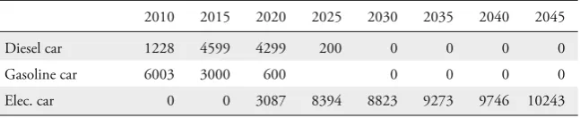
When we restrict severely the GHG emissions, electric cars penetrate strongly from year 2020 on and replace totally the diesel cars in 2030 (see Table 8).

Table 8: Private Transport (1000 kmqVehicle / Day)

2010 2015 2020 2025 2030 2035 2040 2045

Diesel car 1228 4599 4299 200 0 0 0 0

Gasoline car 6003 3000 600 0 0 0 0

Elec. car 0 0 3087 8394 8823 9273 9746 10243

(23)

Figure 14: Energy Consumption by End-Use Sectors (PJ/Y) – BAU Case.

0 10 20 30 40 50 60 70

2005 2010 2015 2020 2025 2030 2035 2040 Others District heating Electricity Oil (transport) Gas

Oil (heat)

Figure 15: Energy Imports (PJ/Y) – BAU Case.

0 5 10 15 20 25 30 35 40 45 50

2005 2010 2015 2020 2025 2030 2035 2040 2045

Others

Diesel for transport Unleaded Gasoline Gas

(24)

Table 9: Electric Vehicle Battery Activity (in PJ). Example in Winter 2040.

Day Night

consumption from network 0 6.40

release of stored electricity 5.88 0

usage for transport 0.82 0.41

usage for storage 0 5.88

usage for network 3.88 0

storage loss (20%) 1.18 0.10

Wind mills and solar PV units penetrate and reach their capacity limit of 500 MW in 2035 (Table 10).

Table 10: Renewable Electricity Capacities (MW)

2010 2015 2020 2025 2030 2035 2040 2045

Photovoltaic 12 15 15 7 3 500 500 500

Wind 1 56 200 300 500 500 500 500

The end-use energy balance shows the progress of electricity consumption (Figure 16). This electricity is mostly obtained by increasing the electricity imports, which is considered carbon neutral in this scenario (Figure 17).

In summary, the factor 4 scenario maximizes the penetration of electricity, using intensively wind, solar and import sources. Electric cars penetrate and contribute importantly to a leveling of demand through a storage activity from night to day.

4.7 Regulation Scenario: Limits on Electricity Imports and CO2 Emissions

(25)

Figure 16: Energy Consumption by End-Use Sectors (PJ/Y) – Factor 4 Case.

0 5 10 15 20 25 30 35 40 45 50

Oil (heat)

Figure 17: Energy Imports (PJ/Y) – Factor 4 Case.

0 5 10 15 20 25 30 35 40

2005 2010 2015 2020 2025 2030 2035 2040 2045 Others

(26)

another possible approach would have been to estimate the carbon footprint of imported electricity and including it in the GHG emission balance.

Table 11: Car Capacities (1000 kmqVehicle per Day)

2010 2015 2020 2025 2030 2035 2040 2045

Diesel car 1228 4599 4299 2215 2311 95 0 0

Gasoline car 6003 3000 600 0 0 0 0 0

Electric car 0 0 3087 6178 6512 9178 9746 10243

As shown in Table 11 the electric car tends to be the major technology used for private transport near the end of the time horizon although it only slowly replaces totally the diesel car usage. This behavior is the consequence of both the mitiga-tion goal and the bounding of imports. To produce more efficiently, one imports electricity during night at low price and distributes the electricity during the day as shown in Table 12.

Table 12: Electric Vehicle Battery Activity (in PJ). Example in Winter 2040.

Day Night

consumption from network 0 3.86

release of stored electricity 3.34 0

usage for transport 0.82 0.41

usage for storage 0 3.34

usage for network 1.84 0

storage loss (20%) 0.68 0.10

In Figure 18 we can observe that the use of electricity remains moderate in the end-use sectors, whereas natural gas replaces totally oil for space heating.

(27)

Figure 18: Energy Consumption by End-Use Sectors (PJ/Y) – Regulation Case.

0 5 10 15 20 25 30 35 40 45 50

Oil (heat)

Figure 19: Energy Imports (PJ/Y) – Regulation Case.

0 5 10 15 20 25 30 35 40 45

2005 2010 2015 2020 2025 2030 2035 2040 2045

Others

(28)

Table 13: Heat Technologies for New Buildings (MW)

2010 2015 2020 2025 2030 2035 2040 2045

Oil furnace 138.9 118 94 76 57 38 19 10

Gas furnace 42 71 87 136 188 209 304 378

Geothermal 0 100 100 100 100 100 100 100

Small CHP 0 66 66 66 66 304 304 310

As a conclusion, imposing the constraints of limited CO2 emissions and lim-ited electricity imports in the same time forces the penetration of local electricity production (wind, solar), efficient heating solutions (CHP) and electric mobility. With respect to the scenario with emissions constraints only, this regulation case favors the co-existence of different technologies, in particular for heat production.

5. Stochastic Analysis

We complement our analysis with a stochastic programming approach based on two uncertain key parameters, (i) the price of electricity imports and (ii) the penetration of electric cars, under the regulation scenario assumptions for other parameters: we consider a constraint on the emissions of 1.75 Mt of CO₂ equiv-alent for all periods, and the import of electricity is bounded to 15 PJ per year.

5.1 Uncertain Parameters and Stochastic Formulation

We focus our stochastic analysis on the import price of electricity and the pen-etration of electric cars. The first parameter is particularly crucial, because the recent decisions on nuclear production taken by several countries will probably lead to an increase of the price of electricity during high demand periods. The programmed closure of the nuclear power plants in 2022 for Germany and in 2034 for Switzerland will modify the electricity imports of these countries and thus affect significantly electricity prices at the european level. To take into con-sideration the uncertainty related to the forthcoming electricity price, we consider a second scenario in which the electricity price in day time-slices grows twice faster from 2025 compared to the first one.

(29)

contrib-7 available for free on http://apps.ordecsys.com/det2sto

8 The deterministic program must be formulated in the GMPL algebraic modeling language (an open source subset of AMPL), and must comply with few conventions. DET2STO automates the formulation of this program via a set of model construction and transformation rules. strongly and ultimately satisfies all or almost all the private transport needs in the Factor-4 or Regulation scenarios. In the stochastic study, we consider two alternative scenarios. In the first one the penetration of electric vehicles is not limited whereas, in the second scenario, electric cars are limited to 25% of the market size observed in the Regulation scenario in 2045. This constraint would represent, e.g., the exogenous effect of non-acceptability of the population due to the fact that an electric car has too low an autonomy.

Combining the uncertainty on the two parameters we end up with a sto-chastic event tree with four scenarios (from SC1 to SC4) that are represented in Figure 20. To generate the stochastic formulation we use the DET2STO7_tool (Dubois, Thénié and Vial, 2005; Thénié, van Delft, and Vial, 2007). This software automatically formulates a stochastic version of a dynamic determin-istic linear program when the uncertainty is described by a simple event tree.8

Figure 20: Event Tree

2010 2025 2050

SC1 Low electricity price

High penetration of electric cars

SC2 Low electricity price

Moderate penetration of electric cars

SC3 High electricity price

High penetration of electric cars

SC4 High electricity price

Moderate penetration of electric cars

(30)

periods 2030–2050. This is the main advantage of this approach over a simple analysis of the different scenarios. It corresponds to the actual situation of a deci-sion maker, which could be summarized by “act and learn’’.

5.2 Analysis of Stochastic Scenarios

In 2020, the electric vehicles penetrate for all scenarios at a moderate level, which corresponds roughly to the bound imposed for the electrical vehicle fleet in sce-narios 2 and 4. In scesce-narios 1 and 3, electric vehicles are used very intensively after 2030. It appears that the main driver of the stochastic analysis is the availi-bility of electric cars, the higher price of electricity having a relatively small impact on electric car penetration (Figure 21) and electricity imports (Figure 22). In Scenario 4, the number of electric cars is restricted and one must invest in other clean technologies to satisfy the emission constraints and consume the stored electricity. Therefore we observe a penetration of electric heat and hot water technologies for houses and buildings. As expected, the constraint on emissions is active for all scenarios.

Figure 21: Activity of Electric Cars (in 1000 kmqVehicle / Day).

2010 2015 2020 2025 2030 2035 2040 2045

12000

10000

8000

6000

4000

2000

0

(31)

Figure 22: Electricity Imports (PJ/Y).

2010 2015 2020 2025 2030 2035 2040 2045 sc1: low price high penetration

sc2: low price mod. penetration sc3: high price high penetration sc4: high price mod. penetration

16

14

12

10

8

6

4

2

0

6. Conclusion

(32)

9 1 Mfr per 1000km q vehicle / day, correponds roughly to 33,000 fr per vehicle, assuming a This modeling exercise is only a first step in the direction of a comprehensive analysis of the potential penetration of renewable technologies in a distribution network in Switzerland, which should evolve toward becoming a smart-grid to permit two-way communication between distributors, producers and consum-ers. Further model developments are needed to integrate a geographical analysis of the capacity limit (upper bound on installed capacities) for solar, wind, and decentralized CHP technologies. In order to properly assess these renewable and smart grid technologies, a more precise representations of the load curve and of transmission and control technologies will be needed. Also the portfolio of tech-nologies has to be enlarged with a greater variety of storage techtech-nologies, includ-ing the pumped storage facilities that are installed in Switzerland and shared by several distributors. A better description of the anticipated investment, opera-tion and maintenance cost is also needed. A more detailed stochastic program-ming analysis, taking into account the possible delays in penetration of the more advanced technologies should be performed. Finally a description of the necessary investment in information and communication technologies (ICT) necessary to support a smart grid development should be added to the model.

7. Annex 1: Investment Cost Assumptions

In Table 14 we report the investment costs for the different space heating tech-nologies considered in the model.

In Table 15 we report the assumed investment costs for the new space heating technologies considered in the model.

In Table 16 we report the investment costs9 for the transport technologies con-sidered in the model.

(33)

T able 1 4 : I nv es tme n t C o st s f or S p ac e He at in g T ec h nolog ie s. ( M fr /G W )

2010 2015 2020 2025 2030 2035 2040 2045

E

xisting buildings

RA1 RA2 RA3 RA4 RA7 RA8 RA9 RAA RAB RAH RAH2

O

il furnace +

WW

O

il furnace

G

as furnace +

WW G as furnace E l. baseboar d heaters

Insulation type 1 Insulation type 2 Insulation type 3 Insulation type 4 District heat RA-1 District heat RA-2

345 342 385 329 731 345 520 780 954 200 200

E

xisting houses

RB1 RB2 RB3 RB4 RB5 RB7 RBA RBD

O

il furnace +

WW

O

il furnace

G

as furnace +

WW G as furnace W ood sto ve E l. baseboar d heaters B iogas furnace D

istrict heat RB

564 512 504 495 741 857 495 533

N ew buildings RC 1 RC 2 O

il furnace +

(34)

2010 2015 2020 2025 2030 2035 2040 2045

N

ew buildings (continued)

3 4 5 7 H

G

as furnace +

WW G as furnace W ood sto ve E l. baseboar d heaters D

istrict heat R

C

311 361 468 573 455

317 370 480 587 461

323 379 491 601 467

328 388 503 616 472

334 397 514 630 478

334 405 525 644 483

345 414 537 658 489

351 423 549 672 489

N

ew houses

O

il furnace +

WW

O

il furnace

G

as furnace +

WW G as furnace W ood sto ve E l. baseboar d heaters B iogas furnace E

l. heat pump _District heat RD

562 611 478 496 778 668 496 ₁₁₈₂ 644

572 624 487 507 795 683 507 ₁₁₈₂ 653

583 638 496 518 812 698 518 ₁₁₈₂ 662

593 651 504 528 829 713 528 ₁₃₀₅ 672

603 665 513 539 846 728 539 ₁₃₀₅ 681

613 678 522 550 863 743 550 ₁₃₀₅ 690

623 691 531 561 880 758 561 ₁₃₀₅ 699

634 705 540 572 897 773 572 ₁₃₀₅ 699

W

arm water buildings

WW solar/elec WW electricity WW gas

598 256 256

W

arm water houses

WW solar/elec WW SFH,electricity WW SFH, solar WW electricity

1300 468 256 1430

(35)

T able 1 5: I n ve st me n t C o st s f or Ne w S p ac e He at in g T ec h nolog ie s. ( M fr /G W )

2010 2015 2020 2025 2030 2035 2040 2045

RA C CHP for buildings unav ailable unav ailable

1000 1000 1000 1000 1000 1000

R CC CHP for ne w buildings unav ailable unav ailable

1000 1000 1000 1000 1000 1000

R CG G eothermal unav ailable unav ailable

1200 1200 1200 1200 1200 1200

T able 1 6 : I nv es tme n t C o st s f or T ra n sp or t T ec h nolog ie s. ( M fr /1 0 0 0 k m q vh c/ d ))

2010 2015 2020 2025 2030 2035 2040 2045

TE1

D

iesel

0.46 0.46 0.46 0.46 0.46 0.46 0.46 0.46

TE2

G

asoline

car

0.43 0.43 0.43 0.43 0.43 0.43 0.43 0.43

TES

E

lectric

car

0.92 0.92 0.92 0.76 0.60 0.60 0.60 0.60

T1R F uel cell car methanol

1.37 1.37 1.37 1.37 1.37 1.37 1.37 1.37

T1S F uel cell car gasoline

1.37 1.37 1.37 1.37 1.37 1.37 1.37 1.37

T1Q F uel cell car hy dr ogen

2.00 2.00 2.00 2.00 2.00 2.00 2.00 2.00

T1T F uel cell car nat. gas

1.37 1.37 1.37 1.37 1.37 1.37 1.37 1.37

TEH1

hy

dr

ogen

car

0.55 0.55 0.55 0.55 0.55 0.55 0.55 0.55

TEM

methanol

car

0.44 0.44 0.44 0.44 0.44 0.44 0.44 0.44

TEN

natural

gas

car

0.50 0.50 0.50 0.50 0.50 0.50 0.50 0.50

T

A1

D

iesel

bus

(36)

2010 2015 2020 2025 2030 2035 2040 2045 Liquid H ydr ogen B us

2.61 2.61 2.61 2.61 2.61 2.61 2.61 2.61

F uel cel bus hy dr ogen

2.61 2.61 2.61 2.61 2.61 2.61 2.61 2.61

F uel cel bus nat. G as

2.61 2.61 2.61 2.61 2.61 2.61 2.61 2.61

F

uel

cel

bus

ethanol

2.68 2.68 2.68 2.68 2.68 2.68 2.68 2.68

B

us

methanol-90%

1.76 1.76 1.76 1.76 1.76 1.76 1.76 1.76

B

us

methanol

100%

1.76 1.76 1.76 1.76 1.76 1.76 1.76 1.76

T

rolleybus

5.13 5.13 5.13 5.13 5.13 5.13 5.13 5.13

tr

uck

diesel

0.67 0.67 0.67 0.67 0.67 0.67 0.67 0.67

deliv . F uel cell ethanol

1.00 1.00 1.00 1.00 1.00 1.00 1.00 1.00

deliv . F uel cell hy dr ogen

1.00 1.00 1.00 1.00 1.00 1.00 1.00 1.00

deliv . T ruck fuel cell nat. G as

1.00 1.00 1.00 1.00 1.00 1.00 1.00 1.00

tr

uck-gasoline

0.58 0.58 0.58 0.58 0.58 0.58 0.58 0.58

M

iscellaneous

1.26 1.26 1.26 1.26 1.26 1.26 1.26 1.26

train

1.26 1.26 1.26 1.26 1.26 1.26 1.26 1.26

tr

uck

methanol

33%

0.19 0.19 0.19 0.19 0.19 0.19 0.19 0.19

tr

uck

diesel

0.18 0.18 0.18 0.18 0.18 0.18 0.18 0.18

tr

uck

fuel-cell

ethanol

0.27 0.27 0.27 0.27 0.27 0.27 0.27 0.27

tr uck fuel-cell hy dr ogen

0.27 0.27 0.27 0.27 0.27 0.27 0.27 0.27

tr uck fuel-cell nat. G as

(37)

T able 1 7: I nv es tme n t C o st s f or C onv er sion T ec h nolog ie s. ( M fr /G W )

2010 2015 2020 2025 2030 2035 2040 2045

E07

P

hoto

voltaic

6000 6000 5000 4000 3000 2000 2000 2000

E08

W

ind

mill

1500 1250 1250 1250 1250 1250 1250 1250

E0D O il-F ir ed Steam-C ycle

1950 1950 1950 1950 1950 1950 1950 1950

E0E

G

as

T

urbine

300 300 300 300 300 300 300 300

E0F G as CC 450 450

450 450 450 450 450 450

ECH

Cheneviers

CHP

12000 12000 12000 12000 12000 12000 12000 12000

E6A

Industrial CHP gas turbine (5 MW

) 800 800 800 800 800 800 800 800 E6B Industrial CHP

. steam turbine (5 MW

) 1000 1000 1000 1000 1000 1000 1000 1000 E6C Ind. CC (5 MW )

1200 1200 1200 1200 1200 1200 1200 1200

E90

ind.CHP

(M

otor)

4160 4160 4160 3640 3640 3640 3640 3640

E9G

comm.

CHP

(M

otor)

5434 5434 5434 4347 4279 4211 4143 4075

E9R

resid.

CHP

(M

otor)

6136 6136 6136 4908 4832 4755 4678 4602

EA3

gas-fir

ed

plant

(HPL)

260 260 260 260 260 260 260 260

EA4 O il-fir ed plant (HPL)

248 248 248 248 248 248 248 248

EB1

G

as

CC

(CHP)

1000 1000 1000 1000 1000 1000 1000 1000

EB2 O il-F ir ed Steam-C ycle

1100 1100 1100 1100 1100 1100 1100 1100

EB3

G

as

fuel

cell

(38)

T

able 1

8

: I

nv

es

tme

n

t C

o

st

s f

or Sm

ar

t G

rid R

el

at

ed T

ec

h

nolog

ie

s.

(

M

fr

/G

W

)

2010 2015 2020 2025 2030 2035 2040 2045

T

B

atter

y

storage

2000

1000

800 700 600 500 500 500

C

fuel

cell

CHP

with

storage

unav

ailable

unav

ailable

1000 1000 1000 1000 1000 1000

fuel

cell

CHP

with

storage

unav

ailable

unav

ailable

(39)

8. Annex 2: Main Equations of the Model

We give here a description in the modeling language code of the most important equations of ETEM.

The objective function is the function that is minimized. It represents the total

discounted cost of the energy system over the horizon. It is the sum of the total discounted investment cost, the total discounted fixed cost and the total dis-counted variable cost minus the total disdis-counted salvage value.

minimize OBJECTIVE :

VAR_OBJINV + VAR_OBJFIX + VAR_OBJVAR - VAR_OBJSAL;

The EQ_OBJINV equation computes the total discounted investment cost.

Tech-nologies investment costs are directly linked to the new capacity of the period. There is no delay between the time when the decision is taken and the time when the technology is installed. The technology life duration must be equal or longer than the duration of the installation period.

subject to EQ_OBJINV :

VAR_OBJINV = sum{t in T, l in L, p in P_MAP[l]}

cost_icap[t,p]*VAR_ICAP[t,l,p]/((1+discount_rate)**(nb_completed_years[t]));

The EQ_OBJFIX equation computes the total discounted fixed cost. Fixed costs

are linked to the total installed capacities of processes.

subject to EQ_OBJFIX :

VAR_OBJFIX = sum{t in T, l in L, p in P_MAP[l]} annualized*cost_fom[t,p]* (sum{t1 in 1..t : t1>=t-life[p]+1 and t1>=avail[p]}

VAR_ICAP[t1,l,p]+fixed_cap[t,l,p]) # capacity[t,p] /((1+discount_rate)**(nb_completed_years[t]));

The EQ_OBJVAR equation computes the total discounted variable cost. Variable

costs are linked to the activities of processes and to the importation and expor-tation of commodities.

subject to EQ_OBJVAR :

(40)

(

sum{s in S}

( sum{l in L, p in P_MAP[l]} cost_vom[t,p] *

sum{c in C_ITEMS[flow_act[p]]} VAR_COM[t,s,l,p,c]/act_flo[p,c] # activity[t,s,p]

+sum{c in IMP} cost_imp[t,s,c] * VAR_IMP[t,s,c] -sum{c in EXP} cost_exp[t,s,c] * VAR_EXP[t,s,c]

+sum{l in L, p in P_MAP[l], c in C_MAP[p]} cost_delivery[t,s,p,c] * VAR_COM[t,s,l,p,c]

) )

/((1+discount_rate)**(nb_completed_years[t]));

The EQ_OBJSAL equation computes the total discounted salvage value that

represents the value that should be assigned to the processes still available at the end of the planning horizon (e.g. when their technical lives exceed the model’s horizon). By omitting this value, too many investments would occur near to the termination of time horizon (end-of-period effect).

subject to EQ_OBJSAL :

VAR_OBJSAL = sum{t in T, l in L, p in P_MAP[l] : t>=avail[p] and t+life[p]>nb_periods+1}

salvage[t,p]*cost_icap[t,p]*VAR_ICAP[t,l,p]/ ((1+discount_rate)**(nb_completed_years[t]));

The EQ_COMBAL equation defines the balance equation of a commodity. It

ensures that, at any time-slices, the supply of the commodity (by importation or production) is equal or greater than the delivery of the commodity (exportation, consumption or demand).

subject to EQ_COMBAL {t in T, s in S, c in C} :

(sum{l in L, p in P_PROD[c] inter P_MAP[l]} VAR_COM[t,s,l,p,c] + if c in IMP then

VAR_IMP[t,s,c] else

0

(41)

sum{l in L, p in P_CONS[c] inter P_MAP[l]} VAR_COM[t,s,l,p,c] + if c in EXP

then VAR_EXP[t,s,c] else

0 else

frac_dem[s,c]*demand[t,c];

The EQ_CAPACT equation defines the relation between activity and total

installed capacity of a process and ensures that the activity is less than the theo-retic upper bound on activity defined by the capacity installed.

subject to EQ_CAPACT {t in T, s in S, l in L, p in P_MAP[l]} :

sum{c in C_ITEMS[flow_act[p]]} VAR_COM[t,s,l,p,c]/act_flo[p,c] # activity[t,s,p] <= avail_factor[t,s,p]*cap_act[p]*fraction[s]*

(sum{t1 in 1..t : t1>=t-life[p]+1 and t1>=avail[p]}VAR_ICAP[t1,l,p]+fixed_cap[t,l,p]); # capacity[t,p]

The EQ_PTRANS equation defines a relation between an input flow and an

output flow of a process, taking into account the efficiency of the energy trans-formation through the process.

subject to EQ_PTRANS {t in T, s in S, l in L, p in P_MAP[l], cg_in in FLOW_IN[p], cg_out in FLOW_OUT[p]:

eff_flo[cg_in,cg_out]>0} :

sum{c_o in C_ITEMS[cg_out]} VAR_COM[t,s,l,p,c_o] =

eff_flo[cg_in,cg_out] * sum{c_i in C_ITEMS[cg_in]} VAR_COM[t,s,l,p,c_i];

The EQ_PEAK equation defines the balance equation of a commodity at peak

time. It ensures that the installed capacity is enough to meet the highest demand in any time-slice, taking into account a reserve margin and adjustments in the average production.

subject to EQ_PEAK {t in T, s in S, c in C} : 1/(1+peak_reserve[t,s,c])*(

sum{l in L, p in P_PROD[c] inter P_MAP[l] : c in C_ITEMS[flow_act[p]]} cap_act[p]*act_flo[p,c]*peak_prod[p,s,c]*fraction[s]*

(42)

# capacity[t,p]

+ sum{l in L, p in P_PROD[c] inter P_MAP[l] : c not in C_ITEMS[flow_act[p]]} peak_prod[p,s,c]*VAR_COM[t,s,l,p,c]

+ if c in IMP then VAR_IMP[t,s,c] else

0 ) >=

sum{l in L, p in P_CONS[c] inter P_MAP[l]} VAR_COM[t,s,l,p,c] + if c in EXP then

VAR_EXP[t,s,c] else

0;

The Capacity transfer equations describe the relationship between the life of

tech-nologies, investments made, capacities available prior to the planning period and finally capacities installed. These constraints provide the dynamical structure to the model. They represent the way installed capacities result from past invest-ments. One has also to take into account what residual capacity still remains available.

subject to Cpt{Tch in TCH, t in T # Start1[Tch] <= t <= Nomb_Per}: Cap[Tch,t] =

sum {tt in max( 1, t-Life[Tch]+1, Start1[Tch] )..t} Inv[Tch,tt]

+

RESID [Tch,t] ;

References

Acha, S., T. Green, and N. Shah (2010a), “Effects of Optimised Plug-In Hybrid Vehicle Charging Strategies on Electric Distribution Network Losses”, in

IEEE PES Transmission and Distribution Conference and Exposition, New

Orleans, USA.

(43)

Distribution Networks”, in IEEE Power and Energy Society General Meeting, Minneapolis, MN, USA.

Berger, C., R. Dubois, A. Haurie, E. Lessard, and R. Loulou (1990), “Assess-ing the Dividends of Power Exchange between Québec and New York State: A Systems Analysis Approach”, International Journal of Energy Research, 14, pp. 253–273.

Brown, James E., Chris N. Hendry, and Paul Harborne (2007), “An Emerging Market in Fuel Cells? Residential Combined Heat and Power in four Countries”, Energy Policy, 35(4), pp. 2173–2186, URL http://dx.doi. org/10.1016/j.enpol.2006.07.002.

Caratti, P., A. Haurie, D. Pinelli, and D. S. Zachary (2003), “Exploring the Fuel Cell Car Future: An Integrated Energy Model at the City Level”, in Urban Transport IX, Proceedings Urban Transport 2003, Ninth International

Con-ference on Urban Transport and the Environment in the 21st Century, 10–12

March 2003 Crete, Greece, L. J. Sucharov and C. A. Brebbia, eds., South-ampton: WIT Press.

Carlson, D., A. Haurie, J.-P. Vial, and D. S. Zachary (2004), “Large Scale Convex Optimization Methods for Air Quality Policy”, Automatica, pp. 385–395.

Drouet, L. and J. Thénié (2009), “An Energy-Technology-Environment Model to Assess Urban Sustainable Development Policies – Reference Manual v.2.1”, Tech. rep., Ordecsys.

Dubois, A., J. Thénié, and J.-Ph. Vial (2005), “Stochastic Programming: The det2sto Tool”, Tech. rep., Logilab, HEC, University of Geneva and Ordec-sys, URL http://www.ordecsys.com/det2sto.

Fourer, R., D. M. Gay, and B. W. Kernighan (1993), AMPL: A Modeling

Language for Mathematical Programming, Duxbury Press, Brooks, Cole

Pub-lishing Company.

Fragnière, E. (1995), Choix énergétiques et environnementaux pour le canton de

Genève, Thesis no 412, Faculté des Sciences Economiques et Sociales,

Uni-versité de Genève, Genève.

Galus, M. D. and G. Andersson (2008), “Demand Management of Grid Con-nected Plug-In Hybrid Electric Vehicles (PHEV)”, in IEEE Energy 2030 Conference.

Hawkes, A.D. and M.A. Leach (2007), “Cost-Effective Operating Strategy for Residential Micro-Combined Heat and Power”, Energy, 32(5), pp. 711–723, URL http://dx.doi.org/10.1016/j.energy.2006.06.001.

(44)

Hirschberg, S., A. Wokaun, and C. Bauer (2005), “Outlook for CO2-Free Electricity in Switzerland, New Renewable Energy Sources”, Energie Spiegel

14, PSI Paul Scherrer Institute.

Howells, M., H. Rogner, N. Strachan, C. Heaps, H. Huntington, S. Kypreos, A. Hughes, S. Silveira, J. DeCarolis, M. Bazillian, and A. Roehrl (2011), “Osemosys: The Open Source Energy Modeling System: An Introduction to Its Ethos, Structure and Development”, Energy Policy. Huang, Xinhong, Zhihao Zhang, and Jin Jiang (2006), “Fuel Cell

Tech-nology for Distributed Generation: An Overview”, in Industrial Electronics,

2006 IEEE International Symposium on, vol. 2, pp. 1613–1618, URL http://

dx.doi.org/10.1109/ISIE.2006.295713.

IEA (2011a), “Energy Prices and Taxes, Second Quarter, 2011”, IEA Energy

Papers, OECD, International Energy Agency.

IEA (2011b), “World Energy Outlook”, IEA Energy Papers, OECD, International Energy Agency.

Kempton, Willett, and Jasna Tomic (2005), “Vehicle-to-Grid Power Funda-mentals: Calculating Capacity and Net Revenue”, Journal of Power Sources, 144(1), pp. 268–279, URL http://dx.doi.org/10.1016/j.jpowsour.2004.12.025. Loulou, R., A. Kanudia, and D. Lavigne (1996), “GHG Abatement in Cen-tral Canada with Inter-Provincial Cooperation”, Energy Studies Review, 8(2), pp. 120–129.

Marnay, C., G. Venkataramanan, M. Stadler, A. Siddiqui, R. Firestone, and B. Chandran (2008), “Optimal Technology Selection and Operation of Commercial-Building Microgrids”, IEEE Transactions on Power Systems, 23(3), pp. 975–982.

Neef, H.-J. (2009), “International Overview of Hydrogen and Fuel Cell Research”, Energy, 34(3), pp. 327–333, URL http://dx.doi.org/10.1016/j. energy.2008.08.014, <ce:title>WESC 2006</ce:title> <xocs:full-name>6th World Energy System Conference</xocs:full-name> <ce:title>Advances in Energy Studies</ce:title> <xocs:full-name>5th workshop on Advances, Inno-vation and Visions in Energy and Energy-related Environmental and Socio-Economic Issues</xocs:full-name>.

OFSTAT-GE (2005–2010), «Annuaire statistique du canton de Genève». Shin-ichi, I. (2010), “Modelling Load Shifting Using Electric Vehicles in a

Smart Grid Environment”, IEA Energy Papers 7, OECD, International Energy Agency.

(45)

Sundberg, J., P. Gipperth, and C.-O. Wene (1994), “A Systems Approach to Municipal Solid Waste Management: A Pilot Study of Göteborg”, Waste

Man-agement and Research, 12(1), p. 73.

Thénié, J., Ch. van Delft, and J.-Ph. Vial (2007), “Automatic Formulation of Stochastic Programs via an Algebraic Modeling Language”, Computational

Management Science, 4, pp. 17–40.

Weidmann, N., R. Kannan, and H. Turton (2012), “Swiss Climate Change and Nuclear Policy: A Comparative Analysis Using an Energy System Approach and a Sectoral Electricity Model”, This issue.

Wene, C.-O. and B. Rydén (1988), “A Comprehensive Energy Model in the Municipal Energy Planning Process”, European Journal of Operational

Research, 33(2), pp. 212–222.

Zachary, D. S., L. Drouet, U-Leopold, and L. Aleluia Reis (2011), “Trade-Offs between Energy Cost and Health Impact in a Regional Coupled Energy-Air Quality Model: The LEAQ model”, Environmental Research Letters, 6.

SUMMARY