R E S E A R C H
Open Access
Application of oil-film interferometry image
post-processing technology based on
MATLAB
Hao Dong
1*and Sihe Chen
2Abstract
The image post-processing technology based on MATLAB was applied in oil-film interferometry to calculate the skin friction coefficient. This method can recognize the bright and dark fringes by the algorithm based on standard deviation, which is efficient and robust. Furthermore, it can process low-quality images and extract fringe spacing by converted grayscale image and the proper sliding window can catch the discrete objectives precisely by multiple selected windows. In addition, the calculation window size can adjust automatically, which improved the robustness of the algorithm greatly. By comparing the experimental results with the numerical results, it is proved that the method of post-processing based on MATLAB can accurately measure the skin friction in hypersonic flow.
Keywords:Oil-film interferometry, Image post-processing, MATLAB, Hypersonic
1 Introduction
The skin friction, which is defined as the local shear stress exerted by a viscous flow on a solid boundary, gives rise to crucially important flow phenomena. It is not only an important physical quantity in the study of fluid mechanics, but also has great practical significance in engineering. For the commercial airliners and trans-port aircraft, the skin friction is the main source of its total drag. As it is reported that once the drag reduces by 1%, the payload would increase by 10% [1], which means an increase of 10 passengers. Therefore, drag re-duction can bring obvious economic and environmental benefits. For hypersonic vehicles, the skin friction ac-counts for 30% of the total drag [2]. Its value is directly related to whether the integrated shape can obtain net thrust, which is one of the key factors to determine the feasibility of the whole scheme of the hypersonic vehicle. It has an important influence on the surface heat flux and thermal protection system of the aircraft [3]. In con-sequence, the accurate measurement of the skin friction, the improvement of flow around the surface, and the
reduction of the drag are of great significance to opti-mizing the aircraft shape.
The skin friction is investigated mainly by numerical simulation by means of computational fluid dynamics (CFD) and measurement with wind tunnel experiment. Measurement of skin friction is important in providing insight into the flow mechanism as well as validation for CFD techniques. Traditionally, skin friction is directly measured by friction balance [4]. Even though friction balance has high precision, there are some disadvantages to this method. It cannot get the local distribution of the skin friction in a specific component. Moreover, the in-stallation of balances may change the local shape and make it difficult to achieve accurate measurement in the joint area or thinner area. Therefore, advanced high-pre-cision surface friction measurement technology must be developed.
Modern optical mechanics uses the optical method to measure the mechanical parameters. In most cases, the mechanical parameters are hidden in the image of the tested object. With the development of technology, modern optical mechanics, as a method and tool, has been applied in many disciplines, such as medicine, sur-veying and mapping, aerospace, and environment [5–7], and has become one of the important experimental approaches to aid engineering practice and scientific * Correspondence:[email protected]
1College of Aerospace Engineering, Nanjing University of Aeronautics and
Astronautics, Nanjing 210016, China
Full list of author information is available at the end of the article
research. Oil-film interferometry skin friction measure-ment is a kind of non-contact optical measuremeasure-ment method. Skin friction is obtained by measuring the thickness variation of the oil film on the surface of the object by optical interference fringes. It has the advan-tage of no interference, no calibration, high resolution,
curved surface measurement, and so on [8]. This
method has been proved to be a feasible technique to measure the skin friction quantitatively. In order to ex-tract the oil thickness information stored in the interfer-ograms, accurate fringe spacing measurements have to be made. In the past years, a number of methods have been proposed. Original methods are tedious, requiring manual measurement of photographs or using an image processor such as Photoshop. The global measurement of the surface (space) and the unsteady flow (time) require improving the acquisition frequency of oil-film interferometry image as much as possible. High-fre-quency oil-film interferometry produces a huge number of interferograms. Therefore, the technique chosen to determine the fringe spacing has to be accurate, com-pletely automated, and rapid. Evidently, it is time that the technique of determining the fringe spacing by com-puter had to be developed to accomplish the fitting of such a large number of interferograms in a reasonable amount of time.
Currently, various computational methods are avail-able for processing the image data of the oil film experi-ments [9–15]. However, these methods still have obvious defects, such as resulting in great errors or requiring ex-tensive pre-processing. Decker and Naughton [10] devel-oped an automated method using a windowed Fourier transform and a correlation technique capable of locat-ing frlocat-inges in an image. But the technique is only able to identify approximately 70% of the fringes in the image. White [11] and Dunn [12] processed the data based on a regression fit of a sinusoidal model and took the period of the data as the indication of the width of the fringes. The problem of regression method is that it uses a string of data to generate only one value. In addition, since the regression would be compromised when there is imper-fection with the pattern of data, or there is a global vari-ation of brightness or contrast between dark and bright fringes, the requirement for quality of database is rather high. On the other hand, Lunte and Schülein [13] and Andrew Baldwin et al. [14] used fast Fourier transform (FFT) to calculate the frequency of oscillation in the data, but this method also encounters similar problems as the regression method since it is as well suffering from the fact that the data is not always the same as ideally predicted. Bottini et al. [15] identified the fringes by binarizing the image and took the middle line of the binarized fringes as the location of bright and dark im-ages. However, this method requires a proper choice to
binarize the data. It is similar to the two methods in-troduced above, in taking the “middle lines” for later calculation of distance; it requires that the light inten-sity of each bright section is symmetric about the peaks. But since the real case is always not so, some bad binarization would strongly affect the accuracy of the final results.
Hence, a new method of the image post-processing based on MATLAB is developed in this work. This method has the advantage that it does not require a very high-quality image. As will be introduced later, it is able to deal with a profile without well-expected pat-tern. Also, it does not require that the image is well cropped, making the images post-processing be easier. In addition to these advantages, the method is also able to overcome the limit of resolution of the image (limit of equipment, such as Camera resolution). As a result, it can generate a measurement for each point separately for each frame, create a contour of the fringe widths, and give a better caption of the local flow patterns, even if the flow is unsteady.
In this paper, the oil-film interferometry was used to measure the skin friction of a flat-plate model in a hypersonic wind tunnel firstly. Then, the interference fringe images captured were automatically processed by the method as described above. In this process, the fringe spacing of the time interval was obtained. Finally, the skin friction at each position was calculated accord-ing to the principle of oil-film interferometry. By com-paring the experimental results with the numerical results, it can be seen that the method of the image post-processing based on MATLAB can accurately measure the skin friction in hypersonic flow.
2 Methods
The thin oil film equation is the basis for determining the wall shear stress from a thin oil film. The theory is first discussed, and then the simulation of oil film as well as the measurement of wall shear stress using interfero-grams is considered. Finally, the image post-processing approach is discussed with its application for experimen-tal data.
2.1 Oil-film interferometry skin friction measurement
The basic equation form of relation between oil film thickness and wall shear stress is shown in Eq. (1) (full derivation can be found in Brown and Naughton’s report [19]).
∂ho ∂t þ
∂ ∂x
τw;xh2o
2μ
þ∂∂ z
τw;zh2o
2μ
¼0 ð1Þ
where ho is the thickness of oil film, τw,x and τw,z are
the wall shear stress components on the surface coordi-natesxandzrespectively, andtis time.
For the one dimensional situation, the changes of wall shear stress on z coordinate can be ignored. Then, Eq. (1) can be rewritten as Eq. (2).
∂ho ∂t þ
∂ ∂x
τw;xh2o
2μ
¼0 ð2Þ
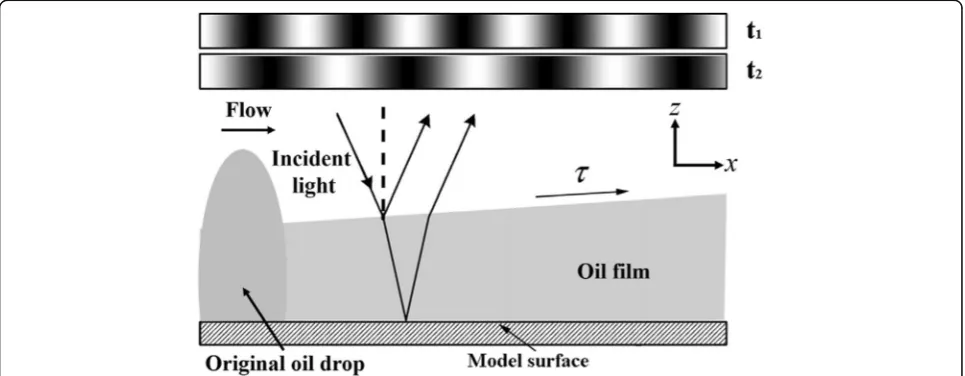
Under the flow and effect of shear stress, the oil be-comes thin. Additionally, illuminated by monochromatic light source, the fringe pattern of oil film can be visible on a reflective surface. Then, the thickness of oil film can be determined by Eq. (3).
ho¼λϕ4π ffiffiffiffiffiffiffiffiffiffiffiffiffiffiffiffiffiffiffiffiffi1 n2
0−sin2θi q
0 B @
1 C
A ð3Þ
whereϕis the phase difference between the portion of the beam reflected from the top of the oil and that transmitted through the oil, n0is the index of reflection of oil, andθiis local illumination angle.
Then, the skin friction can be determined by Eq. (4) according to the solution of Eq. (2) and Eq. (3).
Cf ¼
2n0 cosθrΔx
NλRt2
t1
q∞ð Þt
μð Þt dt
ð4Þ
whereθris the refracted light angle through the oil,λ
is the wavelength of the light source,Nis the number of the fringes used in the equation,Δxis the total width of Nfringes,q∞is the dynamic pressure of the free stream, μ is the viscosity of the oil, and t1 and t2 are the start time and end time, respectively, to capture the pictures.
2.2 Image post-processing
In the present work, a new algorithm based on MATLAB for calculating the space of the oil film fringe is presented. A brief summary of the process of this
algorithm is shown in Fig.2. In this section, an explan-ation for each step is given. In the implementexplan-ation of the algorithm, a MATLAB code is developed.
The image processing includes three main steps. Firstly, the image is pre-processed by converting to grayscale and removing the global brightness variation by subtracting off the local linear trends. Secondly, a proper sliding window is chosen. Within the window, stationarity is assumed; hence, the peaks and troughs, corresponding to dark and bright fringes, can be identi-fied with their deviation from the local mean value. As the fringes are detected, the fringe widths can be deter-mined, which would in turn give an indication to the choice of the window size as well. Finally, with a local filtering, the fringe widths, directly related to the local oil film thickness, can be calculated. The coefficient of friction can be thus calculated from the difference between two images captured in a sufficiently short time interval.
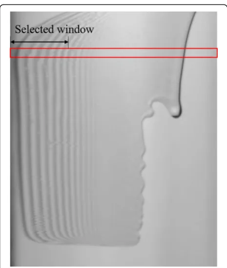
To better illustrate the procedure of the code, as well as to present the advantages of the method, one image from the experiment, as shown in Fig. 3, is used. Note that the x and y axes denote the x and y positions in terms of pixels, respectively. The distinction between bright and dark fringes can be observed clearly from this picture, which can be used for algorithm validation. It can be seen from the picture that it is not well cropped to the specific region of the fringes and gives global brightness variation in transverse direction. Moreover, it can also be seen that the contrast between bright and dark fringes diminishes to the middle part of the image, which indicates that the amplitude of the intensity vari-ation is decreasing.
The pre-processing of the image comes first. Since the bright/dark fringes can easily be identified by the
intensity, the imported image is converted to gray-scale without loss of information. After that, to facili-tate later calculation, a detrending is done to the image. Each row of pixels is divided into sections, and for each section, the local linear fit is subtracted off from the raw data. This step is done for removing the global brightness variation and makes the local variation more distinguishable. In addition, the sec-tions in this step are flexible and can be relatively large, since the global variation of brightness is gener-ally small. After the detrending, an example of one row of the data is shown in Fig. 4, taking the 50th row of pixels in Fig. 3 as the example data. The se-lected section of data is refse-lected in Fig. 3 as the section included in the red frame.
After the pre-processing, we can adopt a rolling-window method to create the contour of the local dis-tances between two neighboring fringes. The principle for the choice of window size is that it should be less than the overall image size, but larger than the dis-tances between fringes. For most of the situations, the local variation would be small enough for using an invariant window size; however, sometimes when the local flow is complex, there may be huge variation. In these situations, the methods based on regression fit would easily fail. However, in the method described in this paper, the problem can be solved by employing an adaptable window size. With the memory of the calculated fringe widths in the neighborhood, the window size could correspondingly be chosen as, for example, three or four times the fringe width. By adjusting the window size automatically, the robust-ness of the algorithm can be greatly improved. After the data is picked out by the window, the calculation is done row by row.
Observation of the data is based on the “peak and trough detection” algorithm. For each row, the mean and standard deviation of the detrended brightness is ex-tracted. If one data point exceeds the mean by more than 0.5 times of the standard deviation, it is marked as a“peak section.” Conversely, if a data point goes below the mean value by more than 0.5 times of the standard deviation, it is marked as a“trough section.”
Thus, for each continuous“peak section,”it is consid-ered as a bright fringe; for each continuous“trough sec-tion,” it is considered as a dark fringe. For each “peak section” or “trough section,” the maximum value or minimum value included in the corresponding data points is taken as the centers of the fringes, which is used for calculation of the distances. The first 101 ele-ments in the series are shown in Fig.4 (right) as an ex-ample (after detrending), with the length of the series taken to be the rolling window size, and the red lines as the limits of detection.
The advantage of this method over the three methods introduced previously can be well illustrated in Fig. 4 (right). It can be inferred from the series of data that it is not necessarily following a sinusoidal trend; on the other hand, the intensity data is not always symmetrical about the peak. Also, some of the dark fringes are with higher intensity in comparison to some of the weaker peaks. Thus, the threshold for binarization appears to be a great difficulty.
Obviously, this method also suffers from noise and in-homogeneity of the input image. Hence, we cannot cal-culate the distance by the simple average of all instances. Instead, the mode of the collection of distances is taken, since the true distance between the fringes is still the most probable value appearing. Since the resolution of the image is limited, the mode itself is not correctly rep-resentative of the true fringe width in the window. Hence, for a better estimation and to show a smooth transition in the contour, the data for this window is taken as the average of mode and the two types of the data taking values of mode+1 and mode−1. When the representative value is calculated, it is stored to be the value for the center of the window. Thereafter, the pos-ition of the window is switched by 1 pixel, thus creating
Fig. 4One detrended row of data and an example of the peak/trough detection algorithm Fig. 3Imported oil film fringe image from the experiment in grayscale.
the contour of all the points (excluding the edge) in the imported image.
After the image is processed, and the local widths of fringes are given, one additional problem arises. The whole graph can be put in, and the regions without oil film would be processed identically. Since the regions generally do not present periodical oscillations, this algo-rithm would not give reasonable values for that region. Hence, some nonsensical values, with great randomness, would be observed in such regions. This fact creates great noise for the created contour, but it also allows optimization of the image by removing noisy regions in the contour. Since the characteristics for the noisy re-gion would differ greatly from case to case due to vari-ous nature of the photo captured. Two methods that can be applied to solve such problems are presented here:
1. Using the entropy of the image. The entropy of the image is defined by its probability distribution of intensity values,− ∑pilog(pi) . Obviously, for those regions with strong noisy and nonsensical values, they would have higher entropy. Hence, a threshold is set, and for all the points with entropy defined by its surroundings exceeding this value in the fringe width plot, we set the value of the point to be zero. This is a more general method but requires some
artificial treatments since a reasonable range of entropy should be defined in advance.
2. Using the probability distribution. This method is relatively simpler but requires that the image is relatively uniform in terms of the fringe widths. Firstly, a probability distribution of fringe width data in the image is calculated. By choosing a certain cluster size, only the data within the range of the most probable cluster are picked. Data out of the range would be abandoned and set to zero. For example, if a window size of 5 pixels is chosen, and the most probable range of the distribution of the pixels is between 10 and 15 pixels, then any data points with a value larger than 15 or smaller than 10 would be set to zero
3 Experiments
3.1 Experimental setup
The present experiments were conducted at the hypersonic wind tunnel in the Nanjing University of Aeronautics and Astronautics (NUAA), see Fig. 5. It is called NHW for short. This is a blow-down and vacuum suction mode wind tunnel which Mach number can be operated from 4.0 to 8.0. The air was supplied by double storage tanks with a volume of 32 m3 at a pressure of 20 MPa. An interchangeable converging-diverging nozzle with an
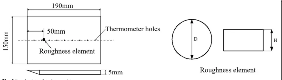
Fig. 6Sketch of the flat plate model
exit diameter of 500 mm was mounted in the plenum chamber. In the downstream of the nozzle, test sec-tion, and diffuser, the air was inhaled into a vacuum ball with a volume of 650m3, and the usable runtime is greater than 10 s. There are two optical windows (300 mm in the diameter) on each side of the plenum chamber for the optical measurements, such as schlieren measurement and particle image velocimetry (PIV) measurement. One rectangular window (300 mm × 350 mm) was opened above the plenum cham-ber for optical access of charge-coupled device (CCD) or high-speed camera. For current experiments, the Mach 5 nozzle was used and the unit Reynolds num-ber is Re= 4.7 × 10⁶m−1 at Ma= 5.0 in order to be consistent with the numerical simulation conditions.
3.2 Test model
The transition from laminar to turbulent flow in a flat-plate boundary layer is one of the most fundamen-tal and often studied subjects in fluid mechanics. Al-though this canonical problem is basic in nature, it can
provide a framework for understanding more complex and practical situations encountered in modern aero-space vehicles.
The model used in the study was a flat plate. It was made of steel with the surface electroplated by the titan-ium to supply the mirror-smooth surface for the oil-film interferometry skin friction measurement. The length of the flat plate isl= 190 mm; the spanwise length isd= 150 mm, which is consistent with the size of the test section of wind tunnel. A cylindrical roughness element was used in the current study with a diameter ofD= 3 mm and height ofk= 1.6 mm. The roughness element adhered to the sur-face of the model at the location of x= 50 mm from the leading edge. During the test, the angle of attack remained atα= 0° and the free stream velocity remained atMa= 5. As the viscosity of silicon oil is related to temperature, the surface temperature of the model should be measured in real time. Temperature measurement is accomplished by placing several T-type thermocouples on the surface of the model to obtain the distribution of temperature. Be-cause of the thinness and thermal properties of silicone
oil, the oil viscosity can be calculated by setting the temperature of silicone oil as that of the sample surface directly [20, 21]. The thermocouples are arranged in the temperature measurement hole. The top of the thermo-couple is flush with the surface of the plate and remains smooth. The diameter of the temperature measurement hole is 1 mm. The sketch of the model is shown in Fig.6.
3.3 Optical path design
The oil applied in the present test was the silicon oil with the viscosity of 50 cSt. The monochrome sodium lamp with the wavelength of 598 nm was used for the il-lumination. Due to the duration of the wind tunnel, the fringe patterns were captured by the HotShot 1280 cc
high-speed camera mounted with the lens of Nikkor AF 70-300 mm f/4-5.6D, with the resolution of 1280 × 1024 pixels. The camera frame rate used in this experiment is 100 frames per second, which is far lower than its shoot-ing speed limit (1000 frames per second).
Figure 7 shows the optical path design of oil-film interferometry experiment in NHW. The plate model is installed in the center of the flow field. Since the high-speed camera cannot be exposed to the vacuum en-vironment of the wind tunnel in the plenum chamber, it shoots the oil-film interferometry fringes through the observation window above the plenum chamber. In order to obtain a wider shooting range of the model surface, the monochrome sodium lamp light source does not directly
Fig. 10Total intensity distribution att= 3 s and 4 s for baseline case
Fig. 12Intensity distribution of oil films #1 and #3 att= 3 s and 4 s for baseline case
shine on the model but reflects on the model surface through the large area of the reflector on upper wall of the plenum chamber. Another advantage of doing so is that it reduces the intensity of incoming light, and the soft monochromatic light makes the fringes clearer.
4 Results and discussion
Figure8shows the baseline oil film patterns taken att= 3 s and 4 s, which are taken without the cylindrical rough-ness element. It can be observed that several oil films dis-tribute along the streamwise, which formed bright and dark fringes. Furthermore, the red rectangle frame is the total data window which can cover all the drops’ fringes (from 60 to 120 mm away from the leading edge).
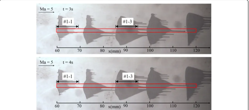
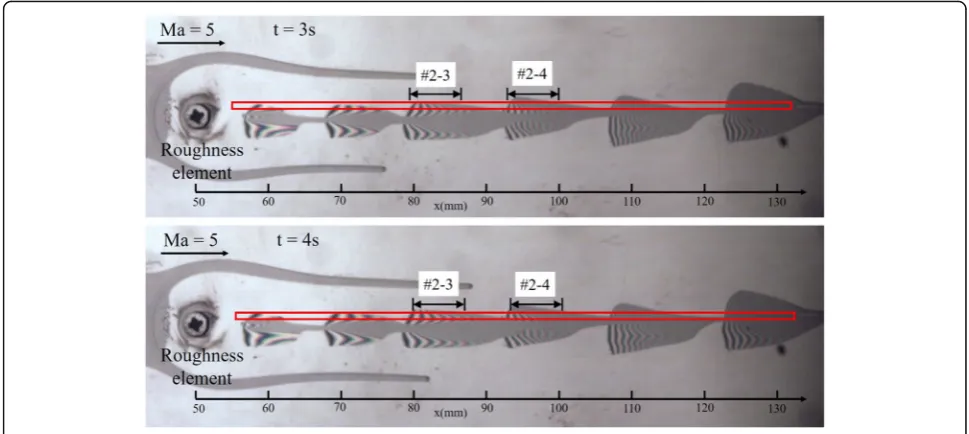
In order to compare with the baseline patterns, the oil film patterns at the same instantaneous for the case with cylindrical roughness element are shown in Fig. 9.
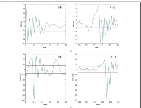
Figure 10 shows the corresponding intensity data ex-tracted from the data selected by the red window as shown in Fig.8, for the baseline case. The intensity dis-tribution of each oil film fringes can be identified clearly (for example, the first #1 and third #3 oil films). Within the oil film fringe region, the intensity distribution shows great amplitude fluctuation comparing with the region without oil film. Similarly, data extracted from the case with the roughness element is plotted in Fig.11,
and the #3 and #4 oil films are taken as examples. It can be observed from the two figures that the presence of the roughness element makes the distance between fringes be varied significantly.
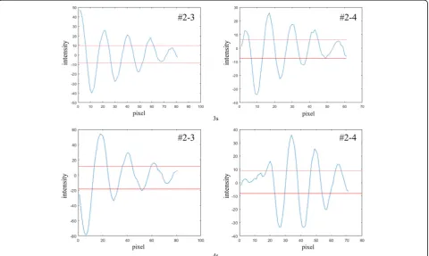
Figure 12 zooms in baseline results of the intensity distribution of oil films #1 and #3 at t= 3 s and 4 s, and Fig. 13 depicts the results with roughness ele-ments, for oil films #3 and #4. For all figures, the red lines represent the detection limits. It can be observed that the intensity in the oil film region is similar to the sine curve, whose peak and valley value corre-sponded the bright and dark fringes respectively. For the baseline case, a fixed window size is used, since the widths of the fringes are basically uniform. In
contrast, as shown in Fig. 11 that the case with
roughness element gives more significant variation, the window size is set locally. In oil film #4, the fringe widths are smaller than that of #3; hence, the smaller window size is adopted for this case. This is to ensure that both overfitting and loss of informa-tion are minimized.
Thereby, the location of every fringe can be identi-fied by the standard deviation method mentioned above. Finally, the Cfof each location can be obtained
by the Eq. (4).
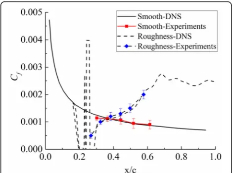
Figure 14 compares the Cf distribution obtained by
experiments and direct numerical simulation (DNS)
[22]. The experimental results agree well with DNS, indicating the validity and accuracy of our processing program. The uncertainty of oil-film interferometry depends on many factors, including oil viscosity, free-stream dynamic pressure, image processing, and some other error sources [23, 24]. In our experiments, it mainly depends on the uncertainty of oil viscosity and image processing. The total uncertainties of the calcu-lation of Cf are plotted in Fig. 14.
5 Conclusion
The image post-processing technology based on MAT LAB was applied in oil-film interferometry to calculate the skin friction coefficient of smooth and roughness flat plate. This method can recognize the bright and dark
fringes efficiently and robustly by the standard
deviation-based algorithm. Furthermore, it can process low-quality images and extract fringe spacing by con-verted grayscale image and the proper sliding window can catch the discrete objectives precisely by multiple se-lected windows. In addition, the calculation window size can adjust automatically, which improved the robustness of the algorithm greatly. By comparing the experimental results with the numerical results, it is proved that the
method of the image post-processing based on
MATLAB can accurately measure the skin friction in hypersonic flow.
Abbreviations
CCD:Charge-coupled device; CFD: Computational fluid dynamics; DNS: Direct numerical simulation; FFT: Fast Fourier transform; NHW: Hypersonic wind tunnel of NUAA; NUAA: Nanjing University of Aeronautics and Astronautics; PIV: Particle image velocimetry
Acknowledgements
The authors would like to thank China Scholarship Council (CSC). This work was funded by CSC to support the first author to conduct this research as an academic visitor in collaboration with the National University of Singapore.
Funding
This research was supported by the National Natural Science Foundation of China (No. 11872208) and Fundamental Research Funds for the Central Universities (No. NP2017202).
Availability of data and materials Please contact author for data requests.
Authors’contributions
All authors take part in the discussion of the work described in this paper. Mr. SC’s main job is writing MATLAB algorithms. Dr. HD is a supervisor of this research and his main job is the wind tunnel experiment and result discussion. Both authors read and approved the final manuscript.
Authors’information
Dr. Hao Dong was born in Luoyang, Henan, P.R. China, in 1983. He received his B. S. in Aircraft Design from Northwestern Polytechnical University in 2005, and his Ph. D. degree in Fluid Mechanics from Nanjing University of Aeronautics and Astronautics in 2010. He is engaged in teaching and scientific research in aircraft design, experimental aerodynamics, and computational fluid dynamics.
Mr. Chen Sihe was born in Pingxiang, Jiangxi, P.R. China, in 1998. He began his persuasion of Bachelor’s degree in National University of Singapore in 2016.
Competing interests
The authors declare that they have no competing interests.
Publisher’s Note
Springer Nature remains neutral with regard to jurisdictional claims in published maps and institutional affiliations.
Author details
1College of Aerospace Engineering, Nanjing University of Aeronautics and
Astronautics, Nanjing 210016, China.2Department of Mechanical
Engineering, National University of Singapore, Singapore 119260, Singapore.
Received: 8 October 2018 Accepted: 20 December 2018
References
1. J. Mullins,Will plasma revolutionize aircraft design. Space Daily(2000) 2. C. Dai, C. Zhang, J. Huang, Hypersonic skin friction stress measurements
using oil film interferometry technique. J. Exp. Fluid Mech.8(2), 68–71 (2012) (in Chinese)
3. J.M. Kendall, Wind tunnel experiments relating to supersonic and hypersonic boundary-layer transition. AIAA J.13(3), 290–299 (1975) 4. J.M. Allen, Improved sensing element for skin-friction balance
measurements. AIAA J.18(11), 1342–1345 (1980)
5. W. Lauterborn, A. Vogel, Modern optical techniques in fluid mechanics. Annu. Rev. Fluid Mech.16(1), 223–244 (1984)
6. M. Kumar, Y.H. Mao, Y.H. Wang, T.R. Qiu, C. Yang, W.P. Zhang, Fuzzy theoretic approach to signals and systems: static systems. Inf. Sci.418, 668–702 (2017)
7. L. Kang, H.L. Du, X. Du, H.T. Wang, W.L. Ma, M.L. Wang, F.B. Zhang, Study on dye wastewater treatment of tunable conductivity solid-waste-based composite cementitious material catalyst. Desalin. Water Treat.125, 296–301 (2018)
8. H.H. Fernholz, G. Janke, M. Schober, P.M. Wagner, D. Warnack, New developments and applications of skin-friction measuring techniques. Meas. Sci. Technol.7(10), 1396 (1996)
9. G. Pailhas, P. Barricau, Y. Touvet, L. Perret, Friction measurement in zero and adverse pressure gradient boundary layer using oil droplet interferometric method. Exp. Fluids47, 195–207 (2009)
10. R.K. Decker, J.W. Naughton, Improved fringe imaging skin friction analysis using automated fringe identification. Paper presented at the 39th AIAA aerospace sciences meeting and exhibit, Reno, NV, U.S.A, 2001 11. J.C. White,High-frame-rate oil film interferometry(Dissertation, California
12. H.M. Dunn,Single camera photogrammetry MATLAB solver developed for automation of the oil interferometry process(Dissertation, California polytechnic State University, San Luis Obispo, 2018)
13. J. Lunte, E. Schülein,Skin friction measurements in three-dimensional flows by white-light oil-film interferometry. New results in numerical and experimental fluid mechanics XI(Springer, Cham, 2018), p. 567
14. A. Baldwin, N. Arora, L. Mears, R. Kumar, F.S. Alvi, J.W. Naughton, Oil film interferometry on the surface under a 3-D flow field. Paper presented at 2018 AIAA aerospace sciences meeting, Kissimmee, Florida, 2018, 15. H. Bottini, M. Kurita, H. Iijima, K. Fukagata, Effects of wall temperature on
skin-friction measurements by oil-film interferometry. Meas. Sci. Technol.
26(10), 105301 (2015)
16. D.M. Driver, Application of oil-film interferometry skin-friction measurement to large wind tunnels. Exp. Fluids34(6), 717–725 (2003)
17. D.M. Driver, G.G. Zilliac, Oil-film interferometry shear stress measurements in large wind tunnels - technique and applications. Paper presented at the 24th AIAA aerodynamic measurement technology and ground testing conference, Portland, Oregon, 2004
18. D.M. Driver, A. Drake, Skin friction measurements using oil-film interferometry in NASA’s 11-foot transonic wind tunnel. AIAA J.46(10), 2401–2407 (2008)
19. J.L. Brown, J.W. Naughton,The thin oil film equation. NASA-TM 1999–208767, NASA-Ames Research Center(1999)
20. J.W. Naughton, M. Sheplak, Modern developments in shear-stress measurement. Prog. Aeosp. Sci.38(6–7), 515–570 (2002)
21. J.D. Ruedi, H. Nagib, J. Osterlund, P.A. Monkewitz, Evaluation of three techniques for wall-shear measurements in three-dimensional flows. Exp. Fluids35(5), 389–396 (2003)
22. Z. Zhu, X. Yuan, L. Chen, Zone decomposition parallel algorithm of high order compact scheme. Chin. J. Comput. Mech.32(6), 825–830 (2015) (in Chinese)
23. G.C. Zilliac,Further developments of the fringe-imaging skin friction technique. Tech. Rep. NASA/TM 110425, NASA-Ames Research Center(1996)