R E S E A R C H Open Access
Measure distorted arrival rate risks and their
rewards
Dilip B. Madan
Received: 16 January 2017 / Accepted: 2 June 2017 /
© The Author(s). 2017Open AccessThis article is distributed under the terms of the Creative Commons Attribution 4.0 International License (http://creativecommons.org/licenses/by/4.0/), which permits unrestricted use, distribution, and reproduction in any medium, provided you give appropriate credit to the original author(s) and the source, provide a link to the Creative Commons license, and indicate if changes were made.
Abstract Risks embedded in asset price dynamics are taken to be accumulations of surprise jumps. A Markov pure jump model is formulated on making variance gamma parameters deterministic functions of the price level. Estimation is done by matrix exponentiation of the transition rate matrix for a continuous time finite state Markov chain approximation. The motion is decomposed into a space dependent drift and a space dependent martingale component. Though there is some local mean reversion in the drift, space dependence of the martingale component renders the dynamics to be of the momentum type. Local risk is measured using market calibrated mea-sure distortions that introduce risk charges into the lower and upper prices of two price economies. These risks are compensated by the exponential variation of space
dependent arrival rates. Estimations are conducted for the S&P 500 index(S P X),
the exchange traded fund for the financial sector(X L F), J. P. Morgan stock prices
(J P M), the ratio ofJPMtoXLF, and the ratio ofXLFtoSPX.
Keywords Variance Gamma·Hunt process·Markov chain approximation·Matrix
exponentiation·Momentum function·Measure distortion
JEL Classification C13·C14·G1·G10·G12
Introduction
Asset prices in financial markets, following Madan and Schoutens (2016b), must change of necessity to support the price with a return for the investor. Furthermore, the changes must be surprises, if all available information has already entered the
D.B. Madan ()
price. As a consequence the changes must occur at surprise times. The simplest model for such times are the arrival times of a Poisson process. The price process is then rendered to be a pure jump process with no continuous component, either determin-istic or random. The process for the logarithm of the price is therefore described by
the structure for the arrival rates of jumps for all jump sizesx,−∞<x<∞.This
arrival rate function may be denoted byk(x,t)where the dependence ontis in all
generality, adapted to all information available at timet.
It was noted in Madan and Schoutens (2016b) that when the local motion is described by the generalized class of limit laws (Khintchine 1938; L´evy 1937; Sato 1999), of which the Gaussian law is an example, that then, in the non-Gaussian limit cases, the integral of the arrival rate function must be infinite. Such processes were termed infinite activity processes in Carr et al. (2002). The random variables at a
finite horizon with arrival rate functions, that only depend on the jump sizex,are
then self-decomposable laws (Sato 1999). The models investigated in the paper are infinite activity processes.
It is then possible for the small jumps to be so frequent as they get smaller that the sum of all the small positive jumps is infinite and the sum of all the small negative jumps is negative infinity. Such processes are called processes of infinite variation. On the contrary, for finite variation processes the sum of all the small positive and negative jumps are separately finite, in any interval. More generally one may take the sum of all positive and negative jumps and their squares to be finite, and not just the small ones. These considerations require that
∞
−∞xk(x,t)d x<∞;
∞
−∞x
2
k(x,t)d x<∞.
The processes being considered for the logarithm of the price are then infinite activity processes of finite variation and quadratic variation.
The use of an infinite activity process is motivated by recognizing that though the number of price moves in reality will be finite it is often quite large for daily data. Such observations inspire the use of limit laws. The limit laws are a special case of infinitely divisible laws termed self decomposable laws with a special structure to their arrival rate functions (Sato 1999). The arrival rate functions when scaled by the absolute jump size must be decreasing functions of the absolute jump size. In particular they are all infinite activity processes.
Finite quadratic variation is a consequence of working with semimartingales that is a maintained hypothesis for arbitrage free price dynamics (Delbaen and Schcharemayer 1994). Finite variation is a simplification that allows one to describe the price process as the difference of two increasing processes, one for the price up ticks and the other for the down ticks. In addition there is considerable evidence (see for a recent example Madan 2016c) that such processes are empirically adequate for describing the physical as well as the risk neutral process.
The stock price processS(t),withX(t)=ln(S(t))then satisfies
X(t)= X(0)+
s≤t
X(s)
Additionally, associated with such a jump process is an integer valued random
measureμ(d x,dt)that counts the jumps occurring in measurable subsets of space
and time. One may then write
X(t)= (x∗μ)t
=
t
0
∞
−∞xμ(d x,ds).
The counting measureμhas a compensatorν(d x,dt)announcing the arrival rate
for jumps at all times that is supposed to be defined by the arrival rate functionk(x,t)
where
ν(d x,dt)=k(x,t)d xdt.
All information about the log price process is then embedded in the arrival rate function and all modeling and estimation efforts are directed to the specification and estimation of arrival rate functions.
In particular there is no room for modeling drifts with or without mean reversion as the price process has no purely deterministic time component. Furthermore, there is also no room for a diffusive volatility given that there is no continuous martingale component in the price process. At the instantaneous level one may only speak of variation and quadratic variation but not directly of drift and volatility. Madan and Schoutens (2016b) shows that the limit of the continuously compounded drift over a
horizonh,denoted by saymt(h)tends on division byh,to the exponential variation.
Specifically, it may be observed that
lim h→0
mt(h)
h =
∞
−∞
ex−1k(x,t)d x.
The concept of reward compensating for risk defined in terms of arrival rate functions is then the exponential variation.
Risk exposures are then measured by the gap between the upper price and the expectation and the expectation less the lower price. Parametric distortions are employed with parameters calibrated to enforce the absence of acceptable opportuni-ties in the options market for the S&P 500 index. The convex and concave distorted physical distribution functions then sandwich the risk neutral distribution of the S&P 500 index. In the continuous time limit probability distortions may be replaced by measure distortions (Madan et al. 2016) of arrival rate functions to construct upper and lower prices and their associated risk exposures. Such option calibrated risk exposures are then observed to be compensated by observed exponential variations across a wide variety of stock days. The result is an alternative asset pricing the-ory based on risk premia for two sided price fluctuations in opposition to classical covariation principles.
Efficient frontiers for risk and reward in terms of multidimensional arrival rate functions are presented in Madan (2016a). Optimal portfolios are here based on max-imizing the lower price of the portfolio. This lower price may also be written as the exponential variation, seen as the reward, less the risk measured by the upper price for the centered and negated risk exposure. The continuous time centering is accomplished by subtracting the exponential variation.
Questions about the presence of local mean reversion or momentum in price pro-cesses are then to be addressed and answered by modeling and estimating arrival rate functions. Such considerations lead us to write arrival rate functions that depend on
both the space variableXand the jump sizex. The data set on which the models will
be estimated are short horizon returns from one to, say, five or ten days and hence time homogeneous models with arrival rate functions that do not specifically depend on calendar time are considered. Pure jump Markov processes with arrival rate func-tions depending on the space variable are called Hunt processes (Hunt 1966). They were formulated and estimated risk neutrally in Madan (2016b) using data on option prices. By way of contrast, the objective of this paper is on their estimation as a physical process from time series data. Mean reversion and momentum are impor-tant aspects of price dynamics influencing responses to abnormal price movements. With strong mean reversion one would sell on an extraordinary uptick while with momentum the appropriate action would be to buy on such upticks. Furthermore the structure of mean reversion and momentum can be different with respect to upward and downward moves and this is commented on in greater detail later. For exam-ples of other applications of Hunt processes in the literature we cite Cont and Minca (2013) and Cousin et al. (2012).
The outline of the rest of the paper is as follows. “Spatially inhomogeneous vari-ance gamma processes” section introduces the spatially inhomogeneous varivari-ance gamma process to be estimated. “Estimation on time series data” section presents two estimation procedures based on matching digital moments and maximum likeli-hood. Results are presented for a variety of asset price time series in “Digital moment estimation result” section. “Drift structure of SIVG” section discusses the structure of mean reversion and momentum in the implied drift structure. “Mean reversion and momentum in the process” section reports on the structure of momentum and mean reversion for the process in aggregate, combining the drift and the martingale components. “Risk compensation” section reports on the implicit risk reward rela-tionships. “The S&P 500 index during the financial crisis” section presents results for the S&P 500 index for the period of the financial crisis covering the years 2007 to 2009. “Conclusion” section concludes this paper.
Spatially inhomogeneous variance gamma processes
The variance gamma processX(t)(Madan and Seneta 1990; Madan et al. 1998) was
originally defined as a Brownian motion with driftθ and volatilityσ time changed
by a gamma process with unit mean rate and variance rateν.For a standard
Brow-nian motionW(t)and a gamma process g(t;ν)the variance gamma process with
parametersσ, ν, θ is
X(t;σ, ν, θ)=θg(t;ν)+σW(g(t;ν)).
The gamma process is a positive increasing process with independent and
identi-cally distributed increments over nonoverlapping intervals of lengthhthat are gamma
distributed with density
f(x)= 1
νhνhν
xhν−1exp−x ν
.
The variance gamma process is a L´evy process with characteristic function
Eexp(i u X(t)) =
1
1−i uθν+σ22νu2
t
ν
.
It is a pure jump process with L´evy densityl(x)parameterized byC,G,M (Carr
et al. 2002) with
l(x)= C
where
C = 1
ν
G = 1
σ
2
ν +
θ2
σ2
+σθ2
M = 1
σ
2
ν +
θ2
σ2
− θ
σ2.
The variance gamma process is a process of finite variation and it can be written as the difference of two increasing process.
The spatially inhomogeneous variance gamma process(S I V G)is constructed by
making the parameters of the variance gamma process in theCGMparameterization
deterministic functions of the space variable to form the jump compensator
νXt(d x,dt)= k(Xt,x)d xdt
= C(Xt)
|x| (1x<0exp(−G(Xt)|x|)+1x>0exp(−M(Xt)x))
for uniformly bounded and positive deterministic functionsC(X),G(X),andM(X).
For details on the existence and uniqueness of the spatially inhomogeneous vari-ance gamma process as a solution to the associated martingale problem described in Stroock (1975) and Stroock and Varadhan (1979), we refer the reader to Angelos (2013). Angelos (2013) follows Bass (1988) to demonstrate the existence and uniqueness of the spatially inhomogeneous variance gamma process.
The specific bounded functions employed, accommodate a local linearity around the current level tapering off to fixed levels at the two extremes. This is accomplished by the use of logistic functions of the form
Y(X)=L+ R−L
1+exp(−ηX)
with parametersL,R,for the left and right limits andηa speed of adjustment. There
are then three parameters in each of the three deterministic functionsC(X),G(X),
andM(X)that we denote byCL,CR,Cη,GL,GR,Gη, ML, MR,and Mη.The
result is a nine parameter spatially inhomogeneous Markov process for the evolution of jumps in the logarithm of the prices.
Defining
δ(X)=
∞
−∞xk(X,x)d x
andμX(d x,dt)as the random measure with compensatorνX(d x,dt),the process for
X(t)may also be written as
d X =δ(X)dt+d[x∗(μX−νX)]t (2)
with a space dependent driftδ(X)and driven by the compensated jump martingale
Apart from mean reversion appearing via the implied driftδ(X),there may be mean reversion or momentum upwards or downwards depending on the dependence
ofGandMonXas well as the presence of leverage via the dependence ofConX.
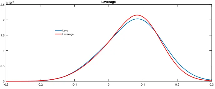
We present graphs comparing a L´evy process to one that endogenized leverage by
raisingCon the down side relative to the up side. For mean reversion and
momen-tum up and down the structure ofM andG responses to the level of the process
may be accordingly adjusted. For mean reversion up, M(X)must rise withX and
fall withX to have momentum up. Similarly for the downside and the dependence
ofGonX.
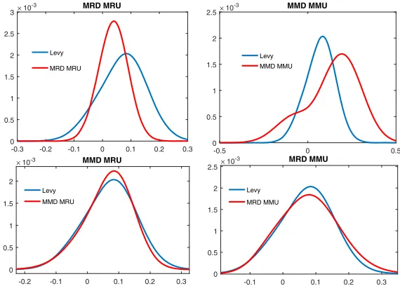
Figure 1 presents a graph for the quarterly return density endogenizing leverage. Figure 2 presents the four cases of mean reversion down and up, momentum down and up, mean reversion down with momentum up, and momentum down with mean reversion up. The construction of the densities is described in the next section.
Estimation on time series data
For the estimation of a spatially inhomogeneous variance gamma process using data on the daily time series of prices, one needs to access the probabilities of returns over various horizons in the model. In this regard, we follow Pistorius and Mijatovic (2011) who show how to approximate a L´e vy process by a continuous time finite state Markov chain and use the approximation to price barrier options. They develop a matrix representation for the infinitesimal generator which on time scaling and matrix exponentiation delivers transition probability elements for the time scales involved. The states of the chain are constructed using a non-uniform grid. The generator is built by integrating the L´evy density between jumps sizes represented by the inter-grid points for the large moves away from the immediate inter-grid on the two sides of a current grid point. The transition rates to the immediate neighbours are built by a diffusion approximation. In the spatially inhomogeneous case considered here, we have a relevant L´e vy density at each grid point with parameters that vary with the
3 . 0 2
. 0 1
. 0 0
1 . 0 -2
. 0 -3
. 0 -0 0.5 1 1.5 2 2.5 10
-3 Leverage
Levy Leverage
5 . 0 0
5 . 0 -0 0.5 1 1.5 2 2.5 10
-3 MMD MMU
Levy
MMD MMU
-0.3 -0.2 -0.1 0 0.1 0.2 0.3 0
0.5 1 1.5 2 2.5
3 10
-3 MRD MRU
Levy
MRD MRU
-0.2 -0.1 0 0.1 0.2 0.3
0 0.5 1 1.5 2
10-3 MMD MRU
Levy
MMD MRU
-0.1 0 0.1 0.2 0.3
0 0.5 1 1.5 2 2.5 10
-3 MRD MMU
Levy
MRD MMU
Fig. 2 Four Cases of Mean Reversion and Momentum on the Up and Down Sides
grid point. The grid is defined with respect to returns and not price levels and the return is always relative to the current stock price of the day.
For the grid, the current spot price is 100 and we employ a 1600 point non-uniform grid ranging from levels 50 to 200 for the spot price. In order to have a substantial variance for the diffusion approximation to the immediate neighbours, the
parame-tersCL,CR are scaled by a thousand. Therefore to build the density at, say,ndays
we scale the generator byn/1000 before evaluating its matrix exponential. The
prob-ability element is constructed at the 1600 return points on matrix exponentiation for one-, five-, and ten-day returns.
-0.02 -0.01 0 0.01 0.02
log return
0 0.2 0.4 0.6
Tail Probability
DME fit to One Day Returns
-0.02 -0.01 0 0.01 0.02
Log Return
0 0.2 0.4 0.6
Tail Probability
MLE fit to One Day Return
-0.04 -0.02 0 0.02 0.04
Log Return
0 0.2 0.4 0.6
Tail Probability
DME Fit to 5 Day Return
-0.04 -0.02 0 0.02 0.04
Log Return
0 0.2 0.4 0.6
Tail Probability
MLE fit to Five Day Returns
-0.05 0 0.05
Log Return
0 0.2 0.4 0.6
Tail Probability
DME Fit to 10 day returns
-0.05 0 0.05
Log Return
0 0.2 0.4 0.6
Tail Probability
MLE fit to 10 Day Returns
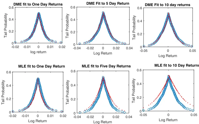
Fig. 3 Digital Moment and MLE fit to tail probabilities for one-, five- and ten-day returns. The observed probabilities are in circles while the estimated model probabilities are represented by dots
moments and maximum likelihood for the one case in which both estimations were conducted.
Digital moment estimation results
The spatially inhomogeneous variance gamma model was estimated for three under-liers, one stock and two indexes, and two ratios of underliers. The stock ticker
was JPM and the two indices were the Exchange Traded Fund for the financial
sector with tickerXLF and the S&P 500 index with ticker S P X.The two ratios
were that ofJPM toXLFandXLFto S P X. In each case the 9 parameters of the
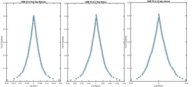
model were estimated. Graphs of the fit of model digital tail probabilities to the observed tail probabilities are also presented. We present in separate subsections the
graphs for the functionsC(X),G(X),andM(X)and the graphs for the fit to tail
probabilities. The data period ranged for a thousand days from August 2, 2012 to July 26, 2016.
JPM
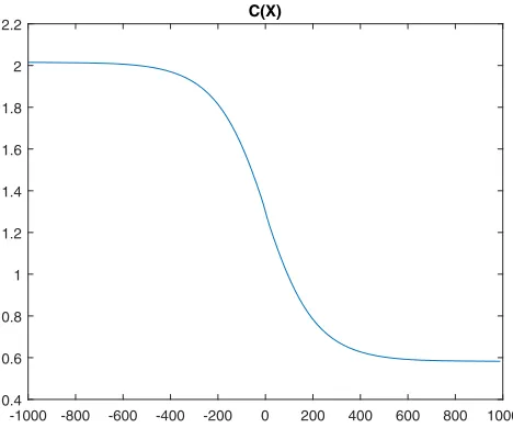
In this caseG,M were independent of X,and Fig. 4 presents a graph of the
func-tionC(X).The constant values forGandM were, respectively, 160 and 143. The
presence of leverage may be observed in the behaviour ofC.
-1000 -800 -600 -400 -200 0 200 400 600 800 1000 0.4
0.6 0.8 1 1.2 1.4 1.6 1.8 2
2.2 C(X)
Fig. 4 The function C(X) for JPM
XLF
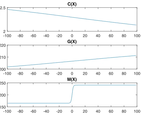
Figure 6 presents the parameters as functions of the log price relative. The behavior
ofC reflects leverage while that ofM andG suggest mean reversion upwards but
momentum downwards in the structure of shocks. Figure 6 presents the function
C(X)over a much narrower range than Fig. 4 and focuses in on the behavior near
zero as opposed to the tails.
Figure 7 presents the graph for the fit to one-, five- and ten-day tail probabilities.
SPX
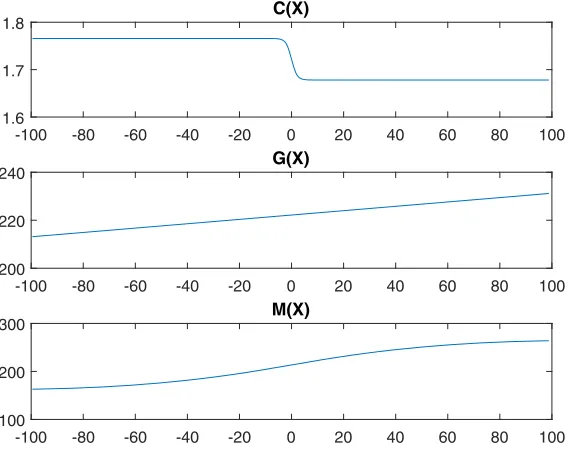
Figure 8 presents the graphs for the parameters as functions of the log price
rela-tive. The general picture is similar toXLFreflecting leverage inC,mean reversion
upwards inMand momentum down inG.
The graph for the fit to one-, five- and ten-day returns is presented in Fig. 9.
-0.04 -0.03 -0.02 -0.01 0 0.01 0.02 0.03 0.04 Return
0 0.1 0.2 0.3 0.4 0.5
0.6 One Day Fit
-0.08 -0.06 -0.04 -0.02 0 0.02 0.04 0.06 Return 0
0.1 0.2 0.3 0.4 0.5
0.6 Five Day Fit
-0.15 -0.1 -0.05 0 0.05 0.1 Return 0
0.1 0.2 0.3 0.4 0.5 0.6
0.7 Ten Day Fit
-100 -80 -60 -40 -20 0 20 40 60 80 100 2
2.5 C(X)
-100 -80 -60 -40 -20 0 20 40 60 80 100
200 210
220 G(X)
-100 -80 -60 -40 -20 0 20 40 60 80 100
150 200
250 M(X)
Fig. 6 The CGM parameters as functions of the log price relative for XLF
JPM2XLF
Figure 10 graphs the parameters as functions of the log price relative for the ratio
ofJPM to X L F.This ratio reflects leverage in C, mean reversion down inGbut
momentum upwards forJPMrelative toX L F.
The fit to one-, five- and ten-day returns is presented in Fig. 11.
XLF2SPX
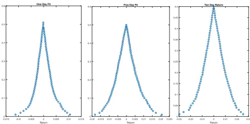
Figure 12 presents the graphs for the parameters as functions of the log price relative.
This ratio reflects a rise in volatility when X L F rises relative to SPX with mean
reversion upwards and momentum downwards.
-0.03 -0.02 -0.01 0 0.01 0.02 0.03 Return
0 0.1 0.2 0.3 0.4 0.5
0.6 XLF Daily Fit
-0.06 -0.04 -0.02 0 0.02 0.04 0.06 Return
0 0.1 0.2 0.3 0.4 0.5
0.6 Five Day Fit
-0.1 -0.08-0.06-0.04-0.02 0 0.02 0.040.06 0.08 Return 0
0.1 0.2 0.3 0.4 0.5 0.6
0.7 Ten Day Fit
-100 -80 -60 -40 -20 0 20 40 60 80 100 1.6
1.7
1.8 C(X)
-100 -80 -60 -40 -20 0 20 40 60 80 100
200 220
240 G(X)
-100 -80 -60 -40 -20 0 20 40 60 80 100
100 200
300 M(X)
Fig. 8 Parameters as functions of the log price relative for SPX
The graphs for the fit to one-, five- and ten-day returns is presented in Fig. 13.
Drift structure of SIVG
The SIVG process inherits all its properties from the structure of the inhomogeneous jump compensator. If we ask, for example, whether there is a limiting stationary dis-tribution, then we need to consider the evolution as described by Eq. (2). Suppose,
-0.03 -0.02 -0.01 0 0.01 0.02 0.03 Return
0 0.1 0.2 0.3 0.4 0.5
0.6 Fit of SPX Daily Return
-0.05 -0.04 -0.03 -0.02 -0.01 0 0.01 0.02 0.03 0.04 Return
0 0.1 0.2 0.3 0.4 0.5
0.6 Five Day Return Fit
-0.08 -0.06 -0.04 -0.02 0 0.02 0.04 0.06 Return
0 0.1 0.2 0.3 0.4 0.5 0.6
0.7 Ten Day Return Fit
-100 -80 -60 -40 -20 0 20 40 60 80 100 0
1
2 C(X)
-100 -80 -60 -40 -20 0 20 40 60 80 100
159.5 160
160.5 G(X)
-100 -80 -60 -40 -20 0 20 40 60 80 100
100 150
200 M(X)
Fig. 10 Parameters as functions of the log price relative for the JPM XLF ratio
for example, we haveδ(X) ≡ 0,then X(t)is a martingale with time independent
compensator. We cannot then have any decrease in forward variances as would be required for convergence to a limiting stationary distribution. Hence the structure
ofδ(X)is critical for the answer to such questions. For the models estimated, on
occasion, we find local mean reversion withδ(X)negatively sloped near zero. Over
a wider range, however, there can be momentum effects withδ(X) > 0 for large
positiveX and negative for large negative X. In some cases we may have global
mean reversion withδ(X) > 0 for X < 0 and the other way around for X > 0.
-0.02 -0.015 -0.01 -0.005 0 0.005 0.01 0.015 0.02 log return
0 0.1 0.2 0.3 0.4 0.5 0.6
Tail Probability
DME fit to One Day Returns
-0.04 -0.03 -0.02 -0.01 0 0.01 0.02 0.03 0.04 Log Return
0 0.1 0.2 0.3 0.4 0.5 0.6
Tail Probability
DME Fit to 5 Day Return
5 0 . 0 0
5 0 . 0
-Log Return 0
0.1 0.2 0.3 0.4 0.5 0.6
Tail Probability
DME Fit to 10 day returns
-100 -80 -60 -40 -20 0 20 40 60 80 100 0
2
4 C(X)
-100 -80 -60 -40 -20 0 20 40 60 80 100
200 400
600 G(X)
-100 -80 -60 -40 -20 0 20 40 60 80 100
0 500
1000 M(X)
Fig. 12 Parameters as functions of the log price relative for the ratio of XLF to SPX
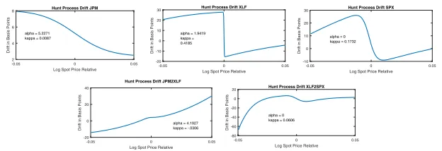
We comment here on the structure of local mean reversion especially if we replace
δ(X)by its local linear approximation to get a non-Gaussian Ornstein-Uhlenbeck
equation (Barndorff-Nielsen and Shephard 2001). Figure 14 presents the five
esti-mated functions forδ(X)along with their local linear approximations. We observe
thatJPM is estimated with mean reversion around an upward trend. X L F, SPX
and the ratio ofXLF to S P X display local mean reversion with global
momen-tum on both sides of the drift. The ratio ofJPM to XLFhas drift momentum on
both sides.
-0.015 -0.01 -0.005 0 0.005 0.01 0.015 Return
0 0.1 0.2 0.3 0.4 0.5
0.6 One Day Fit
-0.02-0.015-0.01-0.005 0 0.0050.010.0150.020.025 Return
0 0.1 0.2 0.3 0.4 0.5
0.6 Five Day Fit
-0.03 -0.02 -0.01 0 0.01 0.02 0.03 Return 0
0.05 0.1 0.15 0.2 0.25 0.3 0.35 0.4 0.45
0.5 Ten Day Return
5 0 . 0 0 5 0 . 0
-Log Spot Price Relative 2
4 6 8
Drift in Basis Points
Hunt Process Drift JPM
5 0 . 0 0 5 0 . 0
-Log Spot Price Relative -20 -10 0 10 20 30
Drift in Basis Points
Hunt Process Drift XLF
5 0 . 0 0 5 0 . 0
-Log Spot Price Relative -10
0 10 20 30
Drift in Basis Points
Hunt Process Drift SPX
5 0 . 0 0 5 0 . 0
-Log Spot Price Relative -20
0 20 40
Drift in Basis Points
Hunt Process Drift JPM2XLF
5 0 . 0 0 5 0 . 0
-Log Spot Price Relative -80 -60 -40 -20 0 20
Drift in Basis Points
Hunt Process Drift XLF2SPX alpha = 5.2271
kappa = 0.0087
alpha = 1.9419 kappa = 0.4185
alpha = 0 kappa = 0.1732
alpha = 4.1927 kappa = -.0306
alpha = 0 kappa = 0.0606
Fig. 14 The functionδ(X)and linear approximations.αis the intercept andκ,when positive, is the rate of mean reversion
Mean reversion and momentum in the process
We evaluate the ratio of the conditional probability for anx% move or greater, down
and up in the next five days, conditional on anx% move down or up just having
occurred to the unconditional probability for such a move. If the conditional prob-ability of an up move rises relative to its unconditional probprob-ability, then we have momentum upwards. Similarly for a down move. If the probabilities of down moves rise conditional on an up move, then we have mean reversion.
Figure 15 presents the ratios of conditional tail probabilities to their unconditional probabilities. The conditional probabilities condition on up and down moves in five days of 50 and 100 basis points for the five estimated models.
We observe, by and large, the presence of momentum. For the ratio of XLF
to SPX the probabilities of large up moves rise on a down move fall on an up
move. Hence there is some mean reversion conditional on large moves in this case. The other cases all support a momentum hypothesis with up and down probabilities rising and the down and up probabilities falling with an up and down move.
-0.08 -0.06 -0.04 -0.02 0 0.02 0.04 0.06 0.08 Size of Jump
0 0.5 1 1.5 2 2.5
Ratio of Post Jump to Pre Jump Probabilities
JPM Momentum Function up 50 down 50 up 100 down 100
-0.08 -0.06 -0.04 -0.02 0 0.02 0.04 0.06 0.08 Size of Jump
0 0.5 1 1.5 2 2.5 3
Ratio of Post Jump to Pre Jump Probabilities
XLF Momentum Function up 50 down 50 up 100 down 100
-0.08 -0.06 -0.04 -0.02 0 0.02 0.04 0.06 0.08 Size of Jump
0 0.5 1 1.5 2 2.5 3 3.5 4
Ratio of Post Jump to Pre Jump Probabilities
SPX Momentum Function up 50 down 50 up 100 down 100
-0.08 -0.06 -0.04 -0.02 0 0.02 0.04 0.06 0.08 Size of Jump
0 5 10 15
Ratio of Post Jump to Pre Jump Probabilities
XLF2SPX Momentum Function up 50 down 100 up 100 down 100
-0.08 -0.06 -0.04 -0.02 0 0.02 0.04 0.06 0.08 Size of Jump
0 1 2 3 4 5
Ratio of Post Jump to Pre Jump Probabilities
JPM2XLF Momentum Function up 50 down 50 up 100 down 100
Risk compensation
Classically, the motion of a stock has been described as a random variable over some horizon with a mean and some volatility. Risk compensation then relates attributes of the random component to the mean return. At the level of surprise moves captured in the arrival rate function there is no mean return to be explained and neither is there a volatility. We only have the arrival rate function. Madan and Schoutens (2016b) shows and the introduction summarized the reward concept to be derived from the arrival rate function as the exponential variation. This is the limiting drift rate for the process that now depends on the spatial variable for a spatially inhomogeneous process. We may then ask what the risk is and how and whether the reward is related to this risk.
In economies satisfying the law of one price, there is a price to be explained and rewards are explained by covariations of returns with the change of mea-sure from probability to price. All events are viewed as having both a price and a probability with a change of measure essentially given by the ratio of the two. It then follows algebraically that excess returns may be related to the covariation of returns with the measure change. Different asset pricing models propose dif-ferent and diverse candidate models for the measure change (see Skiadis (2009) for example).
With financial markets taken to be in a state of continuous and surprising motion the law of one price is suspended as the price is always in a state of flux. Transactions occur at a myriad of prices arising out of negotiations in the process of price discov-ery. We go on instead to consider the possibility of coupling no arbitrage with the fiction of a two price economy, replacing the fiction of the law of one price. In a one price economy the terms of trade are invariant to the direction of trade as one may buy or sell any amount at the going price. Hence zero cost cash flows or cash flows net of their prices form a subspace closed under negation. For two price economies the terms of trade vary with the direction of trade with purchases from market occur-ing at higher prices than sales to the market. The set of zero cost cash flows remains a convex cone but is no longer closed under negation and hence is not a subspace. Under no arbitrage it fails to meet the nonnegative cash flows and convex set separa-tion principles yield a class of measures under which the zero cost cash flows have a nonpositive expectation (see Madan 2015a).
Madan and Schoutens (2016b) investigate the relationship in the economy between exponential variations as reward related to two sided risk concepts based on the shave in value embedded in the lower price and the add-on to value embedded in the upper price. Madan and Schoutens (2016b) show that exponential variations as rewards reflect premia for both of the two sided risk concepts embedded in two price economies. Hence covariation based risk exposures and premia are replaced by explicit risk charges related to the risk of price fluctuations as assessed by the lower and upper prices existing in two price economies.
Here this very same relationship is investigated for the five estimated processes separately, relating spatially contingent exponential variations to the two sided spa-tially contingent risk measures of the lower price shave and the upper price add-on. For the lower and upper price construction one needs to specify the measure dis-tortions. These are the same distortions as employed in the Madan and Schoutens (2016b) study. These distortions were calibrated to bring risk neutral prices embed-ded in option markets to lie within the measure distorted physical arrival rates for
data on theS&P 500 index. Both the option and time series data on index options
were employed for the calibration.
The measure distortions are two increasing concave/convex functions of the pos-itive half line that are bounded below/above by the identity. The specific parametric distortions employed are
+(x)= x+a1−e−cx
1
1+γ
−(x)= x−b
c(1−e −cx).
The values fora,b,c,andγ are 3.1191, 0.9694, 0.3108, and 0.4877.For an arrival
rate functionk(X,x)define the measure of a measurable subsetAof the real line by
K(X,A)=
A
k(X,x)d x.
Now the lower priceL,the exponential variationV,and the upper priceU may
be written as
L = −
∞
0
+KX,ex−
1−> v
dv+
∞
0
−KX,ex−
1+>v
dv
V = −
∞
0 K
X,ex−1−> v
dv+
∞
0 K
X,ex−1+> v
dv
U = −
∞
0
−KX,ex−
1−>v
dv+
∞
0
+KX,ex −
1+> v
dv.
So the risk charge for the shave to lower price is
Also the upper price add-on is
U−V=
∞
0
I−−◦
K(X,[ex−1−>v])
dv+
∞
0 (
+−I)◦K(X,[ex−
1+>v])dv.
If the variation is related to the risk charges with premiaα, β then
V =α (V −L)+β (U−V) .
As a consequence,
V = βU−αL
1+(β−α)
Therefore, a relationship is sought between V,U,L. Conditional on X, the
regression
V(X)=a+bL(X)+cU(X),
is estimated. The estimated values forawere near zero and then solving for α, β
yields
α = − b
1−(b+c)
β = c
1−(b+c).
Table 1 provides the values forα, βfor the five estimated processes.
All the estimated SIVG processes have rewards linearly related to risk as embodied in the lower and upper prices and this is the case whether we work with assets or their ratios. The coefficients reflect the response of exponential variations to tail-risk on both sides. A positive coefficient on the lower price suggests that a rise in the down tail attains return compensation suggestive of mean reversion on the down side. A negative coefficient lowers future returns suggestive of momentum on the down side. Similarly, a negative coefficient on the upper price represents mean reversion on the up side while a positive coefficient reflects momentum on the up side.
The S&P 500 index during the financial crisis
We report here on theSIVGmodel fitted for data on the S&P 500 index for the years
2007 through 2009. Figure 16 presents a graph of the dependence of the parameters
Table 1 Premia for lower shave and upper add-on
Asset α β
JPM 3.3013 −3.2174
XLF −3.9919 3.9366
SPX −2.5735 2.7636
JPM/XLF −0.7864 0.6773
-100 -80 -60 -40 -20 0 20 40 60 80 100 Log Price Relative
0 0.5
1 C(X)
-100 -80 -60 -40 -20 0 20 40 60 80 100
Log Price Relative 0
50
100 G(X)
-100 -80 -60 -40 -20 0 20 40 60 80 100
Log Price Relative 55
60
65 M(X)
Fig. 16 Graphs for the spatial dependence of C, G, and M for the period 2007 to 2009
C,G, and M on the logarithm of the price relative. We observe the presence of
leverage, mean reversion on the down side, and momentum upwards.
The graphs for the fit to one, five and ten day returns are presented in Fig. 17. Figure 18 graphs the drift as a function of the spatial variate presented as a return. Mean reversion is present locally.
Figure 19 presents the momentum function. The momentum though positive is considerably reduced when compared to the non-crisis period.
Finally, we estimated the up and down side risk premia, and they were both posi-tive suggesting a downside mean reversion coupled with an upward momentum. The
values forα,andβwere, respectively, 0.4657 and 0.0012.
Conclusion
The dynamics of movements in prices are modeled as the accumulation of surprise jumps in the logarithm. As a consequence, there are no deterministic time com-ponents or any continuous martingale comcom-ponents. All the information about price changes is embedded in the arrival rate function compensating the surprise jumps.
-0.06 -0.04 -0.02 0 0.02 0.04 0.06 Log Price Relative 0
0.1 0.2 0.3 0.4 0.5 0.6
Tail Probability
One Day Fit
-0.1 -0.05 0 0.05 0.1 Log Price Relative 0
0.1 0.2 0.3 0.4 0.5 0.6
Tail Probability
Five Day Fit
-0.2 -0.15-0.1 -0.05 0 0.05 0.1 Log Price Relative 0
0.1 0.2 0.3 0.4 0.5 0.6
Tail Probability
10 Day fit
-0.1 -0.08 -0.06 -0.04 -0.02 0 0.02 0.04 0.06 0.08 0.1 Spot Log Price Relative
-80 -60 -40 -20 0 20 40 60 80
Drift in Basis Points
SPX 2007-2009
Fig. 18 The drift as a function ofX
A Markov pure jump model is formulated for the motion by making the parameters of the variance gamma L´evy measure deterministic functions of the level of prices. Estimation is conducted by employing a continuous-time finite-state Markov chain approximation that yields probability elements on matrix exponentiation of the transi-tion rate matrix. The dynamics is then decomposed into a space dependent drift and a space dependent martingale component. Though there is some local mean reversion, by and large, the dynamics estimated is that of the momentum type. Risk compensa-tion is estimated via a linear relacompensa-tion between the exponential variacompensa-tion and measure distorted variations for the lower and upper prices of two-price economies. Estima-tions are conducted for the S&P 500 index (SPX), the exchange traded fund for the financial sector (XLF), J. P. Morgan stock prices (JPM), the ratio of JPM to XLF, and the ratio of XLF to SPX.
-0.08 -0.06 -0.04 -0.02 0 0.02 0.04 0.06 0.08
Size of Jump 0.8
0.85 0.9 0.95 1 1.05 1.1 1.15 1.2 1.25
Ratio of Post Jump to Pre Jump Probabilities
SPX Front End Momentum Function
Competing interests
The author declares that he/she has no competing interests.
References
Angelos, B: The Hunt Variance Gamma Process with Applications to Option Pricing. University of Maryland, PhD. Dissertation (2013)
Artzner, P, Delbaen, F, Eber, M, Heath, D: Coherent Measures of Risk. Math. Finance9, 203–228 (1999) Barndorff-Nielsen, O, Shephard, N: Non-Gaussian Ornstein-Uhlenbeck-based models and some of their
uses in financial economics (with discussion). J. R. Stat. Soc. Ser. B63, 167–241 (2001)
Bass, RF: Uniqueness in law for pure jump Markov processes. Probab. Theory Relat. Fields79, 271–287 (1988)
Carr, P, Geman, H, Madan, D, Yor, M: The fine structure of asset returns: An empirical investigation. J. Bus75(2), 305–332 (2002)
Cherny, A, Madan, DB: Markets as a counterparty: An Introduction to Conic Finance. Int. J. Theor. Appl. Finance13, 1149–1177 (2010)
Cont, R, Minca, A: Recovering Portfolio Default Intensities Implied by CDO Quotes. Math. Finance23, 94–121 (2013)
Cousin, A, Cr´epey, S, Kan, YH: Delta-hedging correlation risk. Rev. Deriv. Res15, 25–56 (2012) Delbaen, F, Schachermayer, W: A general version of the fundamental theorem of asset pricing. Math. Ann
300, 463–520 (1994)
Hunt, G: Martingales et Processus de Markov. Dunod, Paris (1966)
Khintchine, AY: Limit laws of sums of independent random variables. ONTI, Moscow, Russian (1938) Kusuoka, S: On Law Invariant Coherent Risk Measures. Adv. Math. Econ3, 83–95 (2001)
L´evy, P: Th´eorie de l’Addition des Variables Al´eatoires. Gauthier-Villars, Paris (1937) Madan, DB: Asset pricing theory for two price economies. Ann. Finance11, 1–35 (2015a)
Madan, DB: Estimating parametric models of probability distributions. Methodol. Comput. Appl. Probab 17, 823–831 (2015b)
Madan, DB, Schoutens, W: Applied Conic Finance. Cambridge University Press, Cambridge (2016a) Madan, DB, Schoutens, W: Conic Asset Pricing and The Costs of Price Fluctuations (2016b). Working
Paper, Robert H. Smith School of Business
Madan, DB: Instantaneous Portfolio Theory (2016a). Available at https://ssrn.com/abstract=2804718 Madan, DB: Momentum and reversion in risk neutral martingale probabilities. Quant. Finan14, 777–787
(2016b). Available at https://ssrn.com/abstract=2251300
Madan, DB: Risk Premia in Option Markets. Ann. Finance12, 71–94 (2016c)
Madan, D, Carr, P, Chang, E: The variance gamma process and option pricing. Eur Financ Rev2, 79–105 (1998)
Madan, DB, Pistorius, M, Stadje, M: On Dynamic Spectral Risk Measures and a Limit Theorem (2016). forthcoming Finance and Stochastics
Madan, DB, Seneta, E: The variance gamma (VG) model for share market returns. J. Bus63, 511–524 (1990)
Pistorius, M, Mijatovi´c, A: Continuously Monitored Barrier Options under Markov Processes. Math. Finance23, 1–38 (2011). Also available at https://ssrn.com/abstract=1462822
Sato, K: L´evy Processes and Infinitely Divisible Distributions. Cambridge University Press, Cambridge (1999)
Skiadis, C: Asset Pricing Theory. Princeton University Press, Princeton (2009)
Stroock, DW: Diffusion processes associated with L ´evy generators. Probab. Theory Relat. Fields32, 209– 244 (1975)