O R I G I N A L A R T I C L E
Probabilistic evaluation of the final moisture content of kiln-dried
lumber using the bootstrap method
Ken Watanabe1• Tomoyuki Hayashi2•Isao Kobayashi1
Received: 1 June 2016 / Accepted: 5 September 2016 / Published online: 22 September 2016
ÓThe Japan Wood Research Society 2016
Abstract This paper presents a probabilistic method of evaluating the final moisture content (MC) of lumber obtained at the end of the kiln-drying process. The final MC data of three different drying tests conducted in past studies were analyzed using the bootstrap method. Target MC was tentatively set below 20 % in the analysis. Two characteristic parameters representing the final MC were estimated with bootstrap confidence intervals. These parameters were the standard deviation (SD) and the per-centage of the population that met the MC requirement of less than 20 % (P20). The histograms of the final MC and the subsequent goodness-of-fit tests revealed that the final MC data of two drying tests did not follow any classical probability distributions, including Normal, Log-Normal, Weibull, and Gamma distributions, thus indicating the need for nonparametric statistics. The uncertainty of the final MC could be evaluated with the estimated SD and P20. After deriving the relationships betweenP20 and the cor-responding probability that P20 is not achieved, we demonstrated how such relationships could provide a kiln operator with information to facilitate better decision-making in optimizing a drying schedule.
Keywords Probabilistic evaluationFinal moisture content Kiln-dryingProbability distributionBootstrap method
Introduction
Lumber drying is one of the most time- and energy-con-suming processes in producing lumber products. As the main purpose of lumber drying is to reduce moisture content (MC) to a specific target value, the final MC that is measured at the end of drying is a primary consideration. In general, a large number of lumber are dried simultaneously in a batch kiln, and in such a condition, considerable variability in the final MC occurs [1]. Consequently, after kiln-drying, a batch may contain an unacceptable number of lumber pieces that do not meet the requirement of the appropriate moisture specification [2]. This outcome can lead to increased costs and the lower rates of lumber recovery.
To check the variability in the MC, most kiln operators select a limited number of test samples from the charge, and measure their MC routinely. The MC information is helpful, for example, at the end of drying process, in determining whether or not he or she should stop the kiln containing thousands of pieces dried simultaneously. However, this judgement relies largely on the operator’s experience, since the MC information sampled from the whole charge involves uncertainty which is difficult to quantify. If the final MC data can be systematically evaluated in a probabilistic way, such as data analysis for structural lumber [3–6], the operator could make an objective and accurate decision in optimizing the drying schedule.
Understanding the final MC distribution is very impor-tant in the probabilistic analysis, because classical
Parts of this report were presented at the 64th Annual Meeting of the Japan Wood Research Society, Matsuyama, March 2014 and the 66th Annual Meeting of the Japan Wood Research Society, Nagoya, March 2016.
& Ken Watanabe
1 Forestry and Forest Products Research Institute, 1
Matsunosato, Tsukuba, Ibaraki 305-8687, Japan
2 The Institute of Wood Technology, Akita Prefectural
parametric statistics is based on the assumption of a specific probabilistic distribution. Rice and Shepard [1] extensively measured the MC of about 3500 eastern white pine (Pinus strobusL.) lumbers from 14 kiln charges that were dried in 7 sawmills. Substantial MC variation existed within a given charge and between kilns at each sawmill, and most of the MC distributions were found to be different from Normal distribution. Milota et al. [7] calculated the final MC distribution of mixed hem-fir species and mountain hemlock (Tsuga mertensiana) using a computer simulation, and showed that a number of slowly drying boards tended to skew the MC distribution toward the right. Tenori and Moya [8] and Moya et al. [9] statistically evaluated a variability in the final MC of kiln-dried lumber from plantations in Costa Rica. In the statistical analysis, the normality assumption was assessed, and positive skewness was found in the distribution [9]. The factors affecting the variability in the final MC of kiln-dried lumber was also examined using Pearson’s correlation matrix [10] and general linear model [11], assuming that the final MC follows a Normal distribution. Numerical stochastic models have been intensively developed to simulate the MC dispersion during and after conventional drying [12, 13] and radio-frequency vacuum drying [14–16]. The developed stochastic models could be used to reproduce the final MC distributions, and some of the simulated distributions had a long right tail [12,14]. The results of the above studies indicate that the final MC does not necessarily follow a normal distribution. However, as far as we know, a comprehensive evaluation of the final MC in relation to probabilistic distribution has not been carried out. Moreover, the final MC data have been assessed using only descriptive statistics, such as mean, standard deviation, coefficient of variation, and the per-centage of the population whose MC is within or without the target MC range. The inference of these parameters has not been attempted at all, which means that no uncertainty assessment of the final MC has been carried out. Therefore, establishing a probabilistic evaluation method of the final MC is an important research endeavor.
The purpose of this study was to develop a probabilistic method by which to evaluate the final MC measured at the end of kiln-drying. The final MC data of three different drying tests conducted in the past works were analyzed using the bootstrap method.
Materials and methods
First, the bootstrap method, a modern computer-intensive statistical method, was introduced and its methodology was briefly described. Second, the probability distributions of the final MC were examined to determine whether the
parametric approach can be used for the analysis. Third, the final MC was evaluated with two characteristic parameters, namely, standard deviation (SD) and the percentage of the population that met the MC requirement (Preq). SD is the population parameter representing the variability of the final MC, whereas Preq is one of the most important indi-cators that have a significant impact on lumber recovery and productivity. The uncertainties of SD and Preq were estimated using the bootstrap method, after which we demonstrated how to integrate the bootstrap estimate into the decision-making related to lumber drying.
Principle of the bootstrap method
The bootstrap was first introduced by Efron [17] as a computer-based simulation method for estimating the standard error of a parameter estimate. Over the next decades, the theory and applications of the bootstrap have been developed [18], and the bootstrap became a very practical approach to making statistical inferences without strong parametric assumptions. The bootstrap is a type of Monte Carlo simulation based on resampling from observed data; its algorithm is briefly described as follows [19].
Suppose that a random sample x¼ ðx1;x2;. . .;xnÞ
from an unknown probability distribution F has been observed and we wish to estimate a parameter of interest h¼sðFÞon the basis of x. For this purpose, an estimate
^
h¼sðxÞ is typically calculated from x. Here, sðÞ is a function by which to measure a parameter estimate, such as mean, median, standard deviation, bias, quantiles, and so on.
Let F^ be the empirical distribution, putting probability 1/n on each of the observed values xi, i¼1; 2; . . .;n. A
bootstrap sample is defined to be a random sample of size n, which is drawn with replacement from F, say^ x¼ ðx
1;x
2;. . .;x
nÞ. The star notation indicates that x
is
not the actual data set x, but rather, a randomized or resampled version of x. Thus, the bootstrap sample x¼ ðx
1;x2;. . .;xnÞconsists of members of the original data set
ðx1;x2;. . .;xnÞ, with some appearing zero times, some
appearing once, some appearing twice, etc.
Corresponding to a bootstrap sample x is the bootstrap replication ofh^given as follows:
^
h¼sðxÞ: ð1Þ
The quantity sðxÞ is the result of applying the same functionsðÞto x as applied to x.
By generating independent bootstrap samples xbðb¼
^
hðbÞ ¼sðxbÞ; b¼1; 2; . . .B: ð2Þ
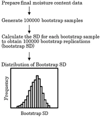
From the distribution of h^ðbÞ, the uncertainty of the parameter estimate h^ can be estimated, for example, by measuring the standard deviation or confidence intervals. A schematic diagram of the bootstrap algorithm is shown in Fig.1.
There are several approaches to construct confidence intervals based on attempts to approximate the per-centiles of the distribution of h^ðbÞ. Efron’s percentile confidence intervals [17] are the two values that cut-off fixed percentages in the tails of the bootstrap distribution of an estimate. For example, the bootstrap 95 % inter-vals are the two values that include 95 % of the boot-strap distribution of an estimate between them. This notion is justified on the basis of the assumption that a transformation exists which can convert the bootstrap distribution of an estimate into a normal distribution [20]. Thus, in small to moderate samples for asymmetric or heavy-tailed distributions, the percentile method is vulnerable [18], and an improved version of the per-centile method called ‘‘bias-corrected and accelerated percentile method’’ (BCa) [21] is required. The BCa adjusts for the median of the distribution of an estimate
that is not equal to the mean and for the standard deviation of the distribution varying with the mean of the distribution. A more detailed description of BCa is provided by Efron [22].
Data preparation
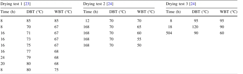
The current study incorporated the final MC data obtained from three different drying tests reported in the literature [23,24]. The drying methods and specimens for each test are briefly described as follows. All the drying tests were conventional kiln-drying tests with schedules listed in Table1. In drying test 3, the second step with a dry-bulb temperature of 120 °C for 18 h represents a high-tem-perature and low-humidity pretreatment, which is effec-tive in preventing surface checks [25]. Next, 222 boards [23], 357 square lumbers [24], and 115 square lumbers [24] were used for drying tests 1, 2 and, 3, respectively. The summary statistics of the final MC data are listed in Table2. In drying test 2, additional drying runs were conducted by Matsumoto and Ishida [24], so the sample size was larger than that in the report. The specific wood species used for the drying tests was sugi (Cryptomeria Japonica).
Fig. 1 Bootstrap algorithm for estimating the uncertainty of parameter estimateh^
Table 1 Drying schedules of the three drying tests
Drying test 1 [23] Drying test 2 [24] Drying test 3 [24]
Time (h) DBT (°C) WBT (°C) Time (h) DBT (°C) WBT (°C) Time (h) DBT (°C) WBT (°C)
8 85 85 12 70 70 8 95 95
8 70 67 168 70 65 18 120 90
16 71 67 168 70 60 504 90 60
16 73 67 168 70 55
16 75 67 168 70 50
16 77 68
24 79 68
20 80 68
8 80 75
Fitting classical probability distributions
Two goodness-of-fit tests, the Kolmogorov–Smirnov test (KS test) and the Anderson–Darling test (AD test), were performed to evaluate whether the final MC data of each drying test followed classical probability distributions. The parameters of each probability distribution were estimated by maximum likelihood, and then subjected to the goodness-of-fit tests. The classical probability distributions employed were Normal, Log-Normal, Weibull, and Gamma distribu-tions. The former three distributions are often used for strength data of structural lumber [3–6], whereas Gamma distribution is a standard probability distribution fitted to continuous data. Moreover, Gamma distribution is used for a random variabley that has positive values, and its proba-bility density function is expressed as follows:
fðy;bÞ ¼ b
a
CðaÞy
a1eyb; ð3Þ
where b is a scale parameter, which is the parameter of interest; a is a known shape parameter; and C(a) is the complete gamma function defined by the following:
CðaÞ ¼ Z 1
0
xa1exdx; a[0: ð4Þ
Horie et al. [3] evaluated the strength data of structural lumber, and used Chi-square test and KS test as goodness-of-fit measures. In the current study, however, the Chi-square test was not used, because the sample data had to be binned before generating the Chi-square test. As we know, the value of the Chi-square test statistic is dependent on how the data are binned. In addition, the Weibull distri-bution employed in this study was not 3P Weibull but 2P Weibull, because the theoretical and physical meanings of the location parameter in 3P Weibull distribution were not clear [3].
Bootstrap estimation of the characteristic parameters for the final MC
The final MC data were evaluated with the two charac-teristic parameters, SD and Preq. In this study, the MC
requirement was tentatively set below 20 %. The SD and P20of the final MC were estimated with 100000 bootstrap replications, and their 95 % confidence intervals were calculated using the BCa method. The procedure to cal-culate the bootstrap SD was shown in Fig.2. Statistical analysis was performed using the MASS package and the boot package in R, version 3.2.3 [26].
Results and discussion
Distribution of the final MC
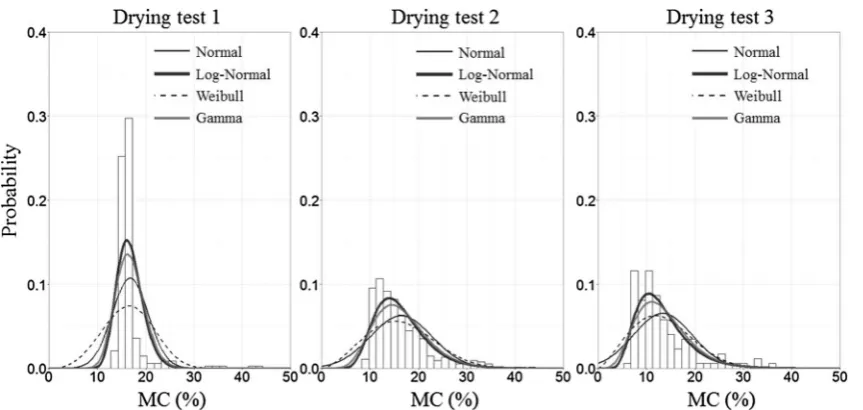
The histograms of the final MC and the fitted probability distributions are shown in Fig. 3. In all the drying tests, the distributions of the final MC had a long right tail. A certain percentage of the population fell above the MC of 30 %. Moreover, these samples remained wet, thereby demon-strating the difficulty in uniformly drying sugi lumber.
To examine whether the final MC data followed the fitted probability distributions (Fig. 3), the goodness-of-fit tests were performed and their results were listed in Table3. In the table, high p values indicate that data probably follow a probability distribution. As can be seen, in the case of drying test 1, the final MC data did not follow any classical probability distribution, which may be attributed to the heavy-tailed nature of the distribution (Fig.3).
In the case of drying test 2, the results of the AD test suggested that all the probability distribution gave a poor fit to the final MC data. Although thep value of the KS test against the Log-Normal null hypothesis was slightly higher than 0.05, this was not enough to ensure that the data Table 2 Summary statistics of the final moisture content for all the
three drying tests
Drying test n Mean (%) SD (%) CV P20(%)
1 [23] 222 16.8 3.7 0.22 92.3 2 [24] 357 16.4 6.4 0.39 80.7 3 [24] 115 13.3 6.1 0.50 89.6
SDstandard deviation,CVcoefficient of variation,P20the percentage
of the population that met the moisture content requirement of less than 20 %
followed the Log-Normal distribution. Thep values in the AD test were consistently lower than those in the KS test. Thus, in evaluating whether the data followed the proba-bility distributions, the AD test tended to judge more conservatively than the KS test.
Meanwhile, in the case of drying test 3, the p values against the Log-Normal null hypothesis were much higher than 0.05 in both the KS test and the AD test. This result implies that the Log-Normal distribution is a good candi-date for the distribution of the final MC of drying test 3.
The histograms of the final MC (Fig.3) and the subse-quent goodness-of-fit tests (Table3) revealed that the final MC data did not necessarily follow a classical probability distribution. Therefore, the conventional parametric statistics are of limited use in evaluating the uncertainty of the final MC. Furthermore, the bootstrap method is thought to be a preferable alternative to parametric statistics.
Bootstrap estimation of characteristic parameters for the final MC
The SD of the final MC was estimated by the bootstrap method (‘‘bootstrap SD’’), and the histograms of bootstrap SD were depicted for each drying test in Fig.4. The uncertainty in the estimated SD can be measured by the histograms. For example, the bootstrap SD for drying test 1 ranged from 1.2 to 6.3 %, whereas the SD of the sample was 3.7 % (Table2). Given that the same drying test was attempted repeatedly, the SD should be within this range. This range can be assessed with confidence intervals in a more probabilistic way. Table4 lists the 95 % BCa con-fidence intervals for the bootstrap SD. The coverage property of this interval implies that 95 % of the time, a random interval constructed in this way will contain the true value [19].
Fig. 3 Histograms of the final moisture content (MC) and fitted probability distributions
Table 3 Results of the goodness-of-fit tests for each drying test
Drying test Goodness-of-fit test Fitted distribution
Normal Log-Normal Weibull Gamma
1 KS test ** ** ** **
AD test ** ** ** **
2 KS test ** 0.064 ** **
AD test ** ** ** **
3 KS test ** 0.462 * 0.139
AD test ** 0.226 ** 0.061
Numbers representpvalues. Thepvalues exceeding 0.05 indicate that null hypothesis was not rejected with 95 % significance level and that the data may probably follow a probability distribution
KS testKolmogorov–Smirnov test,AD testAnderson–Darling test *pvalues less than 0.05
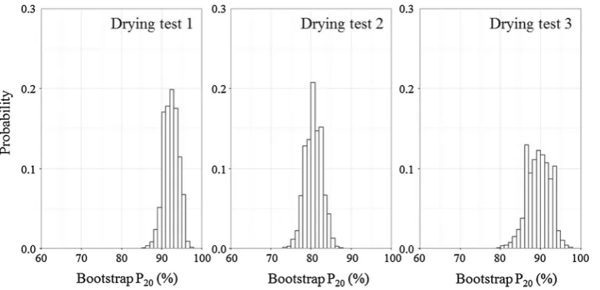
Preq, the percentage of the population that met the MC requirement, is one of the most important indicators that have a significant impact on lumber recovery and produc-tivity. In this study, the MC requirement was tentatively set
below 20 %, and the P20 was estimated by the bootstrap (‘‘bootstrap P20’’). Similar to the estimated SD, the uncertainty in the estimatedP20can also be measured with the 95 % confidence intervals (Table4).
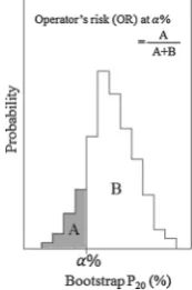
Suppose that a kiln operator wishes to dry at leasta% of the total population within a batch to less than 20 % MC. In other words, a is the acceptable percentage, and the targetP20isa%. The probability that the targetP20ofa% will not be achieved can be estimated from the histograms of the bootstrapP20 in Figs.5 and6. We call this proba-bility ‘‘operator’s risk’’ (OR), which is expressed as follows:
OR¼ProbfP20\ag: ð5Þ
Fig. 4 Histograms of bootstrap standard deviation (bootstrap SD) for each drying test
Table 4 95 % BCa confidence intervals for bootstrap estimates Drying test SD (%) P20(%)
1 2.6–5.3 87.8–95.1
2 5.6–7.7 75.9–84.3
3 5.1–7.5 81.7–93.9
BCabias-corrected and accelerated percentile method,SD standard deviation,P20the percentage of the population that met the moisture
content requirement of less than 20 %
Fig. 5 Histograms of bootstrapP20for each drying test.P20is the percentage of the population that met the moisture content requirement of less
As can be seen in Fig.6, the OR ata% is expressed as the ratio of the area belowa% (A) to the total area (A?B). From Fig.5, the OR was calculated for the whole a to obtain the OR as a function of targetP20(Fig.7). In the case of drying test 1, for example, the OR at 95 and 90 % are 0.92 and 0.09, respectively. This means that 92 % will fail trying to dry 95 % of the total population to less than 20 % MC; in comparison, the risk of failure can be dras-tically reduced to 9 % by changing the P20 from 95 to 90 %. If a kiln operator aims to achieve a target P20 of 95 %, then the current drying operation should be contin-ued to reduce the MC, because the risk of failure is con-sidered to be very high. Meanwhile, if a targetP20of 90 % and the risk of failure of 9 % can be accepted, the kiln operator makes a decision that the current drying operation is working well and should thus be stopped. These results demonstrate that the uncertainty of the final MC could be evaluated using the bootstrap, and that the relationships between the target P20 and the OR could provide a kiln operator with information that can facilitate a better deci-sion-making in optimizing a drying schedule.
The bootstrap method may not be reliable for very small sample sizes, regardless of how many bootstrap samples are generated. Thus, a certain sample size should be acquired. In this study, the sample size of each drying test was more than 100, so a sufficient sample size was pre-pared for the bootstrap analysis.
Conclusions
This study examined the process of evaluating the final MC of lumber obtained at the end of kiln-drying. The goodness-of-fit tests revealed that the final MC data do not neces-sarily follow a classical probability distribution, and that the conventional parametric statistics are of limited use in the probabilistic analysis of the final MC. This is the reason why we utilized the bootstrap method without any assumptions about the underlying probability distribution. The bootstrap method may be suitable for analyzing not only data obtained in the process of lumber drying, but also the strength data of structural lumber, because the sim-plicity of the bootstrap method allows its application in a wide variety of fields.
Our results demonstrated that the bootstrap method is a powerful approach to evaluate the uncertainty and vari-ability of the final MC data. The confidence intervals of SD and P20 were computed from the bootstrap estimates, so that the uncertainty of these parameters could be assessed. Based on the relationships between P20 and the corre-sponding probability thatP20is not achieved, probabilistic risk assessment of the final MC can be implemented in a kiln-drying operation. For example, at the end of drying process, a kiln operator measures the MC of a limited Fig. 6 Schematic diagram of
Fig.5.ORoperator’s risk,a
acceptable percentage,Aarea belowa%,Barea abovea%
Fig. 7 Operator’s risk (OR) as a function of targetP20for each drying test.P20is the percentage of the population that met the moisture content
number of test samples to know if he or she should stop the kiln containing thousands of pieces dried simultaneously. These findings may lead to a higher quality control of kiln-dried lumber.
Acknowledgments The authors would like to thank Dr. H. Mat-sumoto of Forestry Experiment Station, Ishikawa Agriculture and Forestry Research Center for providing the MC data of drying tests 2 and 3.
References
1. Rice RW, Shepard RK (1993) Moisture content variation in white pine lumber dried at seven northeastern mills. For Prod J 43:77–81
2. JAS (1992) Japanese agricultural standard for sawn lumber, sawn balk lumber and sawn lumber with edge. JETRO, Tokyo 3. Horie K, Nakamura N, Iijima Y (1999) Analysis of the strength
data of wood structures on limit states design I. The influence of probabilistic and statistic method on specified values (in Japa-nese). Mokuzai Gakkaishi 45:103–110
4. Horie K, Nakamura N, Iijima Y (1999) Analysis of the strength data of wood structures on limit states design II. Proposal of the method of calculating one-side tolerance limit for weibull dis-tribution (in Japanese). Mokuzai Gakkaishi 45:455–460 5. ASTM D2915-10 (2012) Standard practice for sampling and
data-analysis for structural wood and wood-based products. ASTM International, West Conshohocken
6. ISO 13910 (2005) Structural timber—characteristic values of strength-graded timber—sampling, full-size testing and evalua-tion. International Organization for Standardization, Geneva 7. Milota MR, Morrell JJ, Lebow ST (1993) Reducing moisture
content variability in kiln-dried hem-fir lumber through sorting: a simulation. For Prod J 43:6–12
8. Tenorio C, Moya R (2011) Kiln drying ofAcacia mangiumwild wood: considerations of moisture content before and after drying and presence of wet pockets. Dry Technol 29:1845–1854 9. Moya R, Tovar DA, Tenorio C, Bond B (2011) Moisture content
variation in kiln-dried lumber from plantations of Vochysia guatemalensis. Wood Fiber Sci 43:121–129
10. Mun˜oz F, Moya R (2008) Moisture content variability in kiln-dried Gmelina arborea wood: effect of radial position and anatomical features. J Wood Sci 54:318–322
11. Gu H, Young TM, Moschler WW, Bond BH (2004) Potential sources of variation that influence the final moisture content of kiln-dried hardwood lumber. For Prod J 54:65–70
12. Elustondo D, Avramidis S (2003) Stochastic numerical model for conventional kiln drying of timbers. J Wood Sci 49:485–491 13. Elustondo D, Avramidis S (2005) Comparative analysis of three
methods for stochastic lumber drying simulation. Dry Technol 23:131–142
14. Elustondo D, Avramidis S (2002) Stochastic numerical model for radio frequency vacuum drying of timbers. Dry Technol 20:1827–1842
15. Elustondo D, Koumoutsakos A, Avramidis S (2003) Non-deter-ministic description of wood radio frequency vacuum drying. Holzforschung 57:88–94
16. Elustondo D, Avramidis S (2003) Simulated comparative analysis of sorting strategies for RFV drying. Wood Fiber Sci 35:49–55 17. Efron B (1979) Bootstrap methods: another look at the jackknife.
Ann Stat 7:1–26
18. Chernick MR, LaBudde EA (2011) An introduction to bootstrap methods with applications to R. Wiley, Hoboken
19. Efron B, Tibshirani RJ (1993) An introduction to the bootstrap. Chapman & Hall, New York
20. Manly BFJ (2006) Randomization, bootstrap and Monte Carlo methods in biology, 3rd edn. Chapman & Hall, New York 21. Efron B, Tibshirani R (1986) Bootstrap methods for standard
errors, confidence intervals, and other measures of statistical accuracy. Stat Sci 1:54–77
22. Efron B (1987) Better bootstrap confidence intervals. J Am Statist Assoc 82:171–185
23. Watanabe K, Kobayashi I, Saito S, Hayashi T (2014) Evaluation of the final moisture content of lumber using the bootstrap method (in Japanese). Abstracts of the 64th Annual Meeting of the Japan Wood Research Society, Matsuyama, Japan, 13–15 March, E14-09-1600
24. Matsumoto H, Ishida Y (2015) Influence of different drying conditions on bending strength of Sugi (Cryptomeria japonica) beam with pith (in Japanese). Abstracts of the 65th Annual Meeting of the Japan Wood Research Society, Tokyo, Japan, 16–18 March, E17-P-S09
25. Yoshida T, Hashizume T, Takeda T, Tokumoto M, Inde A (2004) Reduction of surface checks by the high-temperature setting method on kiln drying of Sugi boxed-heart timber without back-splitting (in Japanese). J Soc Mat Sci Jpn 53:364–369