DOI 10.1186/s13408-017-0053-5
R E S E A R C H Open Access
Fundamental Limits of Forced Asynchronous Spiking
with Integrate and Fire Dynamics
Anirban Nandi1 ·Heinz Schättler1· Jason T. Ritt2·ShiNung Ching1,3
Received: 30 January 2017 / Accepted: 25 September 2017 /
© The Author(s) 2017. This article is distributed under the terms of the Creative Commons Attribution 4.0 International License (http://creativecommons.org/licenses/by/4.0/), which permits unrestricted use, distribution, and reproduction in any medium, provided you give appropriate credit to the original author(s) and the source, provide a link to the Creative Commons license, and indicate if changes were made.
Keywords Time optimal control·Spike pattern·Selective spiking
Abbreviations
LIF: Leaky Integrate-and-Fire VP: Victor–Purpura
1 Introduction
The manipulation of networks of neurons in the brain through the use of extrinsic controls—neurocontrol—is a key problem in experimental neuroscience [1]. Such capability has the potential to enable new and important study of questions in neural coding or how the firing activity of brain cells determines their ability to carry and process information [2]. Moreover, improving the use of neurostimulation may aid the refinement of how such technology is used in clinical settings [3,4].
B
A. NandiH. Schättler
J.T. Ritt
S. Ching
1 Electrical and Systems Engineering, Washington University in St. Louis, St. Louis, MO, USA 2 Department of Biomedical Engineering, Boston University, Boston, MA, USA
3 Department of Biomedical Engineering, Washington University in St. Louis, St. Louis, MO,
The use of stimulation in the study of neural coding is itself an established paradigm in neuroscience. The general idea is straightforward: by inducing neural activity and observing the consequent behavior of the organism, we can infer the functional role of the region in question. For example, cortical microstimulation of certain brain regions has been shown to induce behavioral changes in the context of perceptual tasks such as visual decision-making [5,6]. Recently, several key ad-vances in neurostimulation technology, such as the advent of optogenetics [7], have made neurocontrol possible at unprecedented spatial scales. Thus, experimentalists are able to assess the functional role not simply of different neural populations, but potentially of specific neurons and the timing of their spikes. That is, it may be pos-sible to test the long-standing neural coding hypothesis that spike timing is crucial to information processing [8].
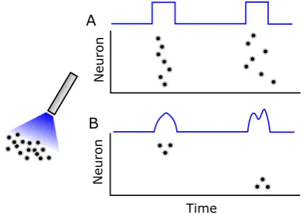
Currently, however, these hardware instantiations are typically used in perturbative paradigms wherein “pulses” of input are used to alter neural firing in a bulk manner (see Fig.1) that does not control the precise timing of individual neuronal spikes. Formal control analysis or design in this context, though desired, is not well studied [9]. Thus, there is a need for formal mathematical analysis regarding the fundamental limits of such stimulation, particularly as it pertains to the feasibility of inducing precisely timed spiking activity in neural populations (Fig.1).
1.1 Prior Work in Neuronal Control
The control of neural activity has received substantial attention in the context of oscillations and synchronization, spurred in large part by interest in clinical brain stimulation for motor disorders [10,11]. The objective in this class of neurocontrol problem is generally the forced splaying of neural phases (i.e., desynchronization),
wherein neurons are typically modeled using phase oscillator formalisms (e.g., [12– 18]). Alternatively, others have approached the problem of desynchronization from the perspective of physiological and instrumentation constraints, favoring methods involving strictly pulsatile stimulation [19–22].
In contrast, we consider herein the mathematical problem of asynchronous neu-rocontrol (i.e., control neural spiking without overt rhythmicity), iIn other words, forcing a neuron to spike but not necessarily periodically. The other key distinction of our work is that we consider a neuronal-level objective (i.e., spiking and spike tim-ing) versus a population-level objective (i.e., synchronization or desynchronization). We have previously provided early formulations of this problem and highlighted key analytical challenges in the development of controllability analysis for spiking mod-els [23,24]. Other works regarding formal control design include optimal control design for a single neuron [25] and using statistical modeling frameworks [26,27].
1.2 Neurocontrol with Common Input
A key challenge associated with neurocontrol is underactuation, wherein a small number of inputs (in many current implementations, a single input) impinges on an orders-of-magnitude greater number of neurons [23], as schematized in Fig. 1. In other words, individual neurons are not addressed via independent inputs, but rather a common one. This challenge is ubiquitous across stimulation modalities and is, perhaps, the major constraint that has restricted the use of neurostimulation to the aforementioned perturbative paradigms. In the context of the discussed oscillatory objectives, some progress has been made on solving control problems such as entrain-ment and synchronization in the presence of underactuation [28–31]. However, this issue is unresolved in the case of asynchronous timed spike control objectives, such as those we consider herein. Current and foreseeable neurostimulation technologies are likely to face the challenge of underactuation, especially for in vivo instantiations.
1.3 Specific Contributions
In this paper, we address the problem of time-optimal control of spiking in pairs of Leaky Integrate-and-Fire (LIF) neurons, where the desired spiking is selective, that is, certain neurons spike while others remain silent. We specifically focus on the case where two neurons receive a common input, which, as mentioned before, is a key con-straint in the practical design of neurocontrol methods. Our major contributions are in the characterization of fundamental limitations for neuron-level control as revealed through a formal mathematical analysis. This treatment leads to the postulation of practical neurocontrol design strategies. Specifically, we provide:
2. The formal synthesis for time-optimal control of longer sequences of spikes. Here, the solution is derived via dynamic programming, but again with several nontriv-ial developments due to nondifferentiability of the value function. In particular, we prove the nonexistence of an optimal solution for specific classes of spike se-quences.
3. The development of design methods for timed patterns of spikes. In this case, there is no unique optimal solution. Nevertheless, we derive a greedy algorithm that can provide near-perfect construction of patterns under specified conditions. Finally, we evaluate the performance of our control design when the system is subjected to noise and disturbances.
Our presentation and discussion on fundamental optimal control analysis and de-sign work toward the overall goal of understanding the limits of neurocontrol. We illustrate several interesting control phenomena that arise due to the peculiarity of spiking dynamics. Specifically, the problem considered, although ostensibly simple, leads to several interesting features in the optimal control synthesis due to state con-straints.
2 Background and Methods
2.1 Definitions: Spike Sequence and Pattern Control
We begin by formally defining the notions of spike sequences and patterns, which will facilitate our approach to spike timing control.
Definition 1 (Spike Sequence) In a population ofN neurons, an M-spike sequence is a vector
ΣS= [σ1, σ2, . . . , σM], (1)
whereσk∈ {1,2, . . . , N}indicates the neuron that produces thekth spike in the
se-quence.
Definition 2 (Spike Pattern) In a population ofN neurons, an M-spike pattern is a sequence with timing, that is,
ΣP =
(σ1, t1), (σ2, t2), . . . , (σM, tM)
, (2)
whereσk∈ {1,2, . . . , N}indicates the neuron which produces thekth spike at time
tk>0, wheret1< t2<· · ·< tM.
The goal of this paper is to provide a set of fundamental characterizations regard-ing the time-optimal control of spike sequences and patterns.
2.2 Model Formulation
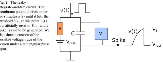
Fig. 2 The leaky
integrate-and-fire circuit. The membrane potential rises under the stimulusu(t )until it hits the thresholdVT, at this pointv(t )
is artificially reset toVrestand a
spike is said to be generated. We also show a cartoon of the possible voltage trace of the neuron under a rectangular pulse input.
2.2.1 Base Model
The integrate-and-fire neuron is a well-established model in computational neuro-science [32,33]. The circuit of this model is shown in Fig.2, where a capacitorC
and resistanceR (modeling the capacitive and resistive properties of the cell mem-brane) are in parallel, withu(t )being the external stimulus. Denoting the membrane potential asv(t ), the charge deposited on the capacitor isq=Cv, and therefore the current is given byIC=Cdvdt, leading to the linear dynamics
Cdv(t )
dt =
Vrest−v(t )
R +βu(t )+Isyn, (3)
whereVrest is the resting potential, andκm=RC is the membrane time constant.
Here,Isyndenotes synaptic input entering from other neurons. We also introduce a
parameterβ that encapsulates the effectiveness of the external inputu(t ) for each neuron.
Spike generation. In this model, a spike is said to be generated at timets if the
membrane potential reaches a predetermined threshold voltageVT. Upon emitting a
spike, the membrane potential is reset toVrest. Thus, spike generation is governed by
the discontinuous resetting rule
vts−=VT → v
ts+=Vrest. (4)
Model normalization. In what follows, we assume thatVrest=0. This normalizing
assumption is not restrictive, since it can be readily achieved by a simple translation in the coordinate system, that is,v←(v−Vrest),VT ←(VT −Vrest).
2.2.2 Synaptic Coupling
We build an approximate model of synaptic coupling based on the standard formu-lations in [33]. Key to this formulation is the notion of impulsive coupling, wherein the major effect ofIsynoccurs during a brief time window following an afferent spike
(i.e., a spike from another neuron). Following a reduction of continuous synaptic models (see AppendixA.1), we formulateIsynas
Isyn(t )=ρsyn(t )
ts∈T
whereT denotes the set of all afferent spike times, andρsyn(t )is a synaptic constant
that depends on the specific parameters of the neuron. If all neurons remain below the threshold, thenIsyn≡0.
Thus, the effect of a synaptic event on the postsynaptic neuron can be understood as an instantaneous rise in voltage that occurs only when a neighboring, connected neuron fires a spike. Knowing this rise can allow us to insulate neurons from each other in the spike control problem, formulated in the next section.
2.3 Problem Formulation: Minimum Time Selective Spiking
In this paper, we study three base problems pertaining to the design ofu(t )to create structured spiking patterns in populations of two LIF neurons of the form (3). We first consider the problem of time-optimal sequence control, that is, inducing target sequences with minimal temporal spacing between the beginning and end of the se-quence. It turns out that this problem amounts to an analysis of selective spiking. We formulate a canonical version of this problem in two dimensions.
Problem 1 (P1: Pairwise time-optimal selective spiking with synaptic guard)
Con-sider two coupled LIF neurons of the form (3):
˙
v1
˙
v2
=
−a1 0
0 −a2
v1
v2
+
b1
b2
u+
Isyn1
Isyn2
≡f (v, u, Isyn)=Av+bu+Isyn, (6)
where v= [v1v2]T,ai=R1 iCi,bi=
βi
Ci,ai, bi>0, andIsyni are impulsive synaptic
inputs of the form (5) fori=1,2. Find the control inputu(t )such that
v1(τ )=VT, v2(t )≤VG< VT, ∀t∈ [0, τ], (7)
with arbitrary initial condition v(0)∈G, where
G= (v1, v2):0≤v1≤VT,0≤v2≤VG
, (8)
andu(t )solves the time-optimization
minimize J(u)=
τ
0
dt (9)
over all measurable functionsuthat take values in the control set, whereUis this set of admissible inputs.
Taken together, (7)–(9) imply that Neuron 1 produces a spike before Neuron 2 and that, under (7), the spike occurs in minimum time.
Functional decoupling of the network via guardVG. The parameterVG in (7),
below threshold and, further, is insulated from the synaptic effect due to the induced spike in Neuron 1, that is,
VG< VT − ¯ρsyn; ρ¯syn=sup t
ρsyn(t ), (10)
whereρsyn(t )is the synaptic contribution to the post-synaptic neuron (here,
Neu-ron 2) and is derived in AppendixA.1. The guard, in essence, keeps the nonselected neuron sufficiently away from its own threshold so as not to produce an undesired, collateral spike.
It is important to note that in solving (P1), it is sufficient to consider the dynamics in (6) as
˙
v=f (v, u,0)≡f (v, u)=Av+bu, (11) since both neurons are below threshold for the duration of the synthesis. Despite this simplification in the dynamics, the selectivity/guard criterion (7) poses a key challenge, that is, it is not sufficient to simply fire Neuron 1 in minimum time, since doing so may in general cause Neuron 2 to fire an undesired spike. Mathematically, (7) functions as a state constraint that, as we will see, leads to several complications in the optimal synthesis.
If the problem has a solution for either choice of neuron labeling, then the pop-ulation is said to be pairwise feasible, that is, either neuron can be made to spike selectively.
Problem 2 (P2: Pairwise time-optimal selective sequencing) For the two-neuron
net-work in (11), find the control input that achieves anyM-spike target spike sequence
ΣStime optimally, that is,
minimize
u∈U J(u)=
τ1
0
dt+ · · · +
τM
τM−1
dt (12)
such that
vσk(τk)=VT,
vσkˆ (t )≤VG, ∀t∈ [τk−1, τk],v(0)∈G,σˆk=Ω\σk,whereΩ= {1,2},
k=1, . . . , M,andτ0=0.
(13)
The key complication here is the nondifferentiability of the value function within the dynamic programming, as well as the spike discontinuity (4).
Problem 3 (P3: Pairwise time-optimal selective patterning) Considering the same
model in (11), find the control that induces the spiking in the two neurons according to the times specified in the target patternΣP, constrained by the underlying sequence.
Mathematically,
minimize
u∈U J
(u)=
M
k=1
(tk−tk−1)−
τk
τk−1
dt
2
with the same constraints as described in (13) andt0=τ0=0. Note thattk are the
desired spike times, andτkare the actual spike times.
3 Minimum Time Selective Spiking
We consider the minimum-time selective spiking problem P1. We assume, without loss of generality, that the neurons are labeled so that the objective is to fire Neuron 1. It turns out that the solution to this problem depends on the ratio (see AppendixA.2)
γ1=
b1a2
b2a1
, (15)
which we treat in two separate cases corresponding toγ1≶VTVG.
As we will show in the following sections, forγ1>VTVG, that is, Case 1, selective
spiking can always be accomplished. However, ifγ1≤VTVG, that is, Case 2, a solution
may not exist, and pairwise feasibility is not guaranteed.
3.1 Selective Spiking, Case 1:γ1>VVTG
Proposition 1 Consider the two-neuron network (11), where
γ1>
VT
VG
. (16)
Assume that the set of admissible controlsU forms a box constraint of the formU=
[0, U], and we take as given the initial conditionsvi(0) < VG,i=1,2. The time
optimal feedback controlu∗∈U for the selective spiking problem P1 for Neuron 1 is given by
u∗=
U forv2< VG,
uarc forv2=VG,
(17)
whereuarc=ab2
2VGis the unique control that keepsv2(t )=VGinvariant. Moreover, such a control always exists. Thus, optimal controls are either given by a constant control at maximum value,u∗(t )≡U, if the state space constraint does not become
active, or if the corresponding trajectory meets the state space constraint, then opti-mal controls are a concatenation of a segment for the maximum control until the state constraint is reached followed by a constant boundary controlu∗(t )=uarcuntil the
terminal valuev1=VT is reached.
Proof Necessary conditions for optimality for problem P1 are given by the
through a direct construction and then verify the optimality of the synthesis. In partic-ular, there is no need to consider possible degeneracies that in principle are allowed by necessary conditions for optimality (e.g., abnormal extremals, etc.).
Synthesis Construction. We want to solve the optimal control problem P1 on the
setGin (8). We first treat the problem in the absence of the state constraint and define the Hamiltonian function as
H(λ,v, u)=1+λ·f (v, u)=1+λ·(Av+bu). (18) According to the maximum principle, as long as no state space constraints are active, the multiplierλis a solution to the adjoint equation
˙
λ(t )= −λ(t )A, (19)
and the optimal control minimizes the Hamiltonian over the control set[0, U]. The
solutions of (19) are of the form
λ1(t )=c1ea1t, λ2(t )=c2ea2t (20)
for some constantsc1andc2, and thus
u∗NoGuard(t )=
U ifΦ(t ) <0,
0 ifΦ(t ) >0, (21)
with
Φ(t )=b1λ1(t )+b2λ2(t ) (22)
as the switching function. The terminal constraint is defined byψ (τ,v)=v1(τ )−VT,
and the transversality condition [34, Sect. 2.2] of the maximum principle implies that
λ(τ )= [ν 0]whereνis some multiplier. This gives usc2=0, and thus the switching
function has a constant sign in the absence of the guard constraint. Hence the optimal control is simply a BANG, that is, the maximal input.
With the state constraint (the guard), there can be switching in the optimal control, and we need to consider two subcases: trajectories that do or do not hit the boundary
v2=VG. For A with real eigenvalues, the optimal controls of linear single input
control systems are BANG-BANG with at most n−1 switchings (wheren is the dimension of the system; heren=2) [34], and we must haveu >0 at the spike time (otherwise, v would be decaying). We thus consider controls only of the form
u=
0 fort≤ ˆtwherev1(t ) < Vˆ T,
U fort < tˆ ≤τ . (23)
These define a smooth flow of extremal controlled trajectories as long as the state space constraint is not violated. If the extremals hit the state constraint boundary, then the control must switch to the boundary controluarcthat keeps the system from
exceeding the constraint:
uarc=
a2VG
b2
However, we need to verify whether this boundary controluarcwill eventually bring
Neuron 1 to threshold. Forv1=VT andu=uarc, we have
˙
v1= −a1VT +b1
a2VG
b2
>0, (25)
where the inequality holds by our assumption onγ1. Now, if (25) holds, then in fact
˙
v1>0 for allv1∈ [0, VT]under the boundary control, andv1will eventually reach
threshold.
Thus for appropriate initial conditions, applying the maximal inputu(t )=U pro-duces a spike in Neuron 1 without hitting the Neuron 2 guard. For the remaining initial conditions, we construct a control that applies maximal input until the guard is reached and then drops touarcuntilv1hits threshold. Note that we do not need to
employ the zero control in (23), so we may taketˆ=0 (the possibility of additional switching will arise in the next section under the alternative case forγ1). Thus the
control (17) will produce a spike in Neuron 1 without inducing a spike in Neuron 2 across all initial conditions. This concludes the synthesis construction.
Proof of Optimality. The optimality of this control follows from regular
synthesis-type sufficient conditions for optimality, and we briefly outline the reasoning. The value or cost-to-go function of this synthesis is continuous but not differentiable on the curve that separates initial states for which the trajectory includes a boundary segment from those that do not. The curveΓ that separates these two regions is defined by the set of initial conditions that hit the final condition v(τ )= [VT VG]T
under the BANG controlu(t )=U. To find this curve, we first explicitly compute the time forv1to hit threshold,
τ = 1 a1
log b1
a1U−v1(0)
b1
a1U−VT
≡ 1
a1
logEv1(0)
−1
, (26)
where for convenience we define
E(v)=
b1
a1U−VT
b1
a1U−v
. (27)
We then eliminateτ by solving explicitly forv2(t )with the final conditionv2(τ )=
VG
VG=E
v1(0)
a2
a1v2(0)+b2
a2
U1−Ev1(0)
a2
a1, (28)
to find the separatrix as
Γ =
v∈G:E(v1) a2
a1v2+b2
a2
U1−E(v1) a2
a1−VG=0
. (29)
We define the regionΓ−as bounded betweenΓ andv1=VT inclusive, and the region
The value function corresponding to this synthesis is
V=
V−(v) for v∈Γ−,
V+(v) for v∈Γ+. (30)
For trajectories without a boundary arc, the value is just the spike time under maximal input, calculated as in (26),
V−(v)= 1 a1
logE(v1)−1
. (31)
The calculation of the valueV+(v)involves two steps: the timetg for Neuron 2 to
reach the guard voltage, plus the timetth for Neuron 1 to attain the threshold VT
under the boundary arc control. By direct calculation,
V+(v)=tg+tth
= 1
a2
log b2
a2U−v2
b2
a2U−VG
+ 1
a1
log b1
a1uarc−v1(tg)
b1
a1uarc−VT
, (32)
where
v1(tg)=
b2
a2U−VG
b2
a2U−v2
a1
a2
v1+
b1 a1 U 1− b2
a2U−VG
b2
a2U−v2
a1
a2
(33)
is the Neuron 1 voltage at the timetg, that is, when the trajectory hits the Neuron 2
guard.
It is clear from the construction thatVis continuously differentiable in the interior ofGaway from the curveΓ. We now show that onΓ,Vremains continuous, but is no longer differentiable. Substitutingv2from (29) into (33) yields
v1(tg)=
VT −ba1
1U
v1−ba1
1U
v1+
b1
a1
U
1−VT −
b1
a1U
v1−ba1
1U
=VT. (34)
Hence (32) reduces to
V+(v)=tg=
1
a2
log
v
2−ba2
2U
VG−ba22U
. (35)
Substitutingv2once again into (35), it follows that V+(v)= 1
a1
logE(v1)
=V−(v). (36)
However,
∂V+ ∂v2Γ
=∂V−
∂v2Γ
so thatVis not continuously differentiable.
All controlled trajectories in the synthesis are extremals, and away fromΓ, the value function V satisfies the Hamilton–Jacobi–Bellman equation for the uncon-strained optimal control problem
∂V(t,v) ∂t +
∂V(t,v) ∂v f
t,v, u∗+Lt,v, u∗=0, (38) whereLis the Lagrangian of the problem (for time optimal control problems, as in our case,L=1).
This conclusion follows from the method of characteristics (e.g., see [34]) but can also directly be verified using the explicit formulas derived above. That V is not differentiable onΓ does not invalidate the proof of optimality, although the stan-dard optimality argument based on dynamic programming (e.g., [34], Theorem 5.2.1) does not apply. Here, we need to invoke regular synthesis constructions (see Ap-pendixA.3) as they are described in [34, Sect. 6.3]. Since trajectories do not return from the state space constraint into the interior of the state space, these arguments could, for example, be undertaken by redefining the state space constraint as a second terminal manifold, along with a penalty term that gives the time along the boundary control untilv1=VT. Alternatively, the constructions in [35], where a regular
synthe-sis argument has been generalized to problems with order 1 state space constraints, could be modified to apply to cases where the state space constraint is active at the terminal time. Either way, straightforward modifications of regular synthesis type
ar-guments give the optimality of the above field of extremals.
Example 1
We demonstrate minimum spike time control in an example of (11) with the fol-lowing parameters:
R1=0.5 GΩ, R2=0.33 GΩ,
C1=300 pF, C2=300 pF,
VT =30 mV, VG=27 mV
U=2.5 nA, β1=1, β2=1.2.
(39)
Note that these are idealized parameters used for illustrative purposes only, although with biologically plausible units. Here, the condition γ1> VTVG is satisfied, and we
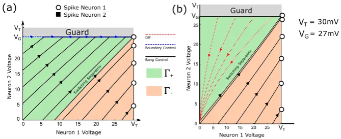
can apply the above proposition to induce a spike in Neuron 1 in minimal time. Fig-ure3(a) shows the state space under this construction.
3.2 Selective Spiking, Case 2:γ1≤VVT
G
We now consider the case of eliciting a spike in Neuron 1 whenγ1≤VTVG.
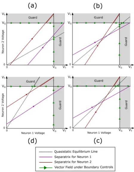
Fig. 3 (a) State trajectories for selective spiking of Neuron 1 under Case 1 for several initial conditions. Trajectories either reach threshold under maximal input, or reach the guard under maximal input and then follow the boundary under a lower constant input until Neuron 1 reaches threshold. (b) State trajectories for selective spiking under Case 2 for several initial conditions. For those trajectories that do not reach Neuron 1 threshold (before hitting the guard) under maximal input, the input is zero until the trajectory decays to the switching separatrix, and then bangs high until Neuron 1 spikes.
We might expect the solution in Case 2 to be qualitatively similar to Case 1, but in fact there are no longer increasing trajectories that ride along the guard boundary: under the boundary control (uarc=a2bVG
2 ), we findv˙1<0 atv1=VT, that is, along
the guard,v1(t )does not rise beyond a certain limit and fails to reach the threshold
VT. Instead, we have the following:
Proposition 2 Consider the two-neuron network (11), whereγ1≤ VVGT. Assume that
the set of admissible controls is a box constraintU= [0, U]. The time optimal control
u∗∈U for the selective spiking problem P1 for Neuron 1, if such a solution exists, is
u∗=
0 for v∈Γ+,
U for v∈Γ−, (40)
withΓ±defined as before.
Proof We follow a similar analysis to the previous case, but identify the differences
in the optimal control structure from the solution in Sect.3.1. Again, our approach is to define a synthesis of extremal controlled trajectories, prove their optimality, and finally give conditions for the existence of a solution for all v∈G.
Synthesis Construction. The Hamiltonian and multiplier are similar to (18) and (20). The minimum condition similarly results in (21) with the conclusion that the optimal control is simply BANG at u∗(t )=U for trajectories that do not hit the guard under this control. Similarly to (28), there again exists a curveΓ that separates such initial conditions from those requiring switching, given by (29). Note that there is no boundary segment in this case asuarccannot drive the voltage of Neuron 1 up
led to consider controls only of the form
u=
0 fort <tˆwherev1(t ) < Vˆ T,
U fortˆ≤t≤τ , (41)
in the interior ofG, andtˆ=0 is allowed. This concludes the synthesis construction.
Proof of Optimality. The value function for the regionΓ−equals the time taken by Neuron 1 to reach the thresholdVT under the constant controlUand takes the same
form as (31). For v∈Γ+, the value function is calculated assuming that the control is turned off for an interval[0,tˆ], during which the system decays from the initial
condition v(0)= [v1v2]T to a point v(t )ˆ = [ˆv1vˆ2]T on the curveΓ. At this time the
control switches to the maximum valueU, and the corresponding trajectory follows the curve until the terminal condition v(τ )= [VT VG]T is reached. This gives
V+(v)= ˆt+tth=
1
a1
log
v1
ˆ
v1
− 1
a1
logE(vˆ1)
, (42)
where
ˆ
v2=
ˆ
v1
v1
a2 a1
v2 and
E(vˆ1)ˆ
v1
v1
a2 a1
v2+
b2
a2
U1−E(vˆ1) a2
a1−VG=0 (43)
using the fact that [ˆv1 vˆ2]T lies on Γ. Here we cannot get an explicit expression
forV+in terms of the initial condition[v1v2]T because of the transcendental form
of (43).
Note that, for this synthesis, the state space constraint does not become active. It is clear from the construction that the corresponding values satisfy the Hamilton– Jacobi–Bellman equation away from Γ. However, this problem is nonstandard in that the value function may no longer be continuous onΓ, with the only exception at
v1=0, that is,
V+(v)=V−(v) for v∈Γ such thatv1=0. (44)
Existence of Solution. However, the control approach in (41) will fail if trajectories starting inΓ+ do not in fact hit the separatrix at some time during the initial off-control. A necessary and sufficient condition for trajectories to hit the separatrix is thatΓ intersects the positivev2axis. When this condition holds and v(0)lies above
Γ, then there must be a timetˆwhere the trajectory hitsΓ underu=0. Conversely, supposeΓ does not intersect the positivev2axis. The slope ofΓ, consideringv2as
a function ofv1, must be less than the slope of the decaying trajectory for there to
be an intersection (ignoring the degenerate parameter choice for which tangency is possible). Taking the ratiosv˙2/v˙1 foru=0 andu=U (recalling thatΓ is itself a
solution with maximal input) and rearranging the result show that the slope condition can be met only ifv2> γ1v1. However, by our assumptionγ1≤VT/VG, no point
onΓ meets this inequality (the curve lies entirely below the line from the origin to [VT VG]T). In fact, sincev˙i,i=1,2, is monotonic inu, it follows that there is no
admissible control that can push a solution acrossΓ, so that the latter serves as a barrier to Neuron 1’s threshold for all initial conditions inΓ+(at least, without first crossing the Neuron 2 guard). So in this case, selective spiking of Neuron 1 is not possible.
Thus, the condition for the existence of a time-optimal solution for selective spik-ing of Neuron 1 is that thev2intercept ofΓ is positive, which occurs when
1−a1VT
b1U
a2
>
1−a2VG
b2U
a1
. (45)
Example 2 We use the same parameter values as in (39) but swap the roles of Neu-ron 1 and NeuNeu-ron 2, that is,
R2=0.5 GΩ, R1=0.33 GΩ,
C2=300 pF, C1=300 pF,
VT =30 mV, VG=27 mV,
U=2.5 nA, β2=1, β1=1.2.
(46)
Now,γ1≤VT/VG. Moreover, condition (45) holds, so that the switching separatrix
intersects the positivev2axis. Thus a time-optimal solution for selectively spiking
Neuron 1 always exists. Figure3(b) shows example trajectories.
3.3 Geometric Interpretation of Cases and Pairwise Feasibility
Thus far in our discussion we assume, without loss of generality, that a selective spike is desired in Neuron 1. Now for pairwise feasibility, that is, to analyze when time-optimal selective spiking of either neuron is possible (from any initial condition), both neurons must be associated with either Case 1 or Case 2. To do this, we introduce
γ2=
b2a1
b1a2
= 1
γ1
. (47)
We associate Neuron 1 withγ1and Neuron 2 withγ2to determine the case (Sects.3.1
orγ1≤VVGT, respectively, and similarly for Neuron 2 with the same inequality relation
onγ2. Since we haveVT > VG, this allows for three possible scenarios,
1. γ1>VTV G,γ2<
VT
VG: Neuron 1 is Case 1, and withγ2being the reciprocal ofγ1, we
have Neuron 2 is Case 2.
2. γ1<VTVG,γ2>VGVT: Neuron 1 is Case 2 and Neuron 2 is Case 1, and the structure
of the solution is identical to the previous scenario. 3. γ1≤VVT
G,γ2≤ VT
VG: Both Neurons are Case 2, and this happens when VG
VT ≤γ1,2≤ VT
VG.
As we will show in the following sections, for one of the neurons belonging to Case 1, pairwise selective spiking can be accomplished. However, ifγ1,2≤VTVG, that is, both
neurons are Case 2, a solution may not exist, and pairwise feasibility is not guaran-teed.
To provide an additional geometric interpretation (see Appendix A.2) of these conditions, we introduce the quasi-static equilibrium line
v(∞):= (v1, v2)|b2a1v1=b1a2v2
, (48)
which defines the set of points for whichv˙=0 (for eachu∈U).
In a pair of neurons, the following two possible parameterization scenarios can be encountered.
3.3.1 Neuron 1 and 2 Correspond to Different Cases
Here we discuss the pairwise feasibility for when Neuron 1 is Case 1 and Neuron 2 is Case 2. It is important to note that the result extends to the reverse scenario, that is, Neuron 1 is Case 2 and Neuron 2 is Case 1.
Here, the line of quasi-static equilibrium in (48) intersects the linev1=VT before
it intersectsv2=VG. Thus, Neuron 1 can always increase along the Neuron 2 guard
boundary. Conversely, Neuron 2 cannot increase along the Neuron 1 guard beyond the point of intersection between v(∞)andv1=VG. As we showed before, in this case,
selective spiking of Neuron 1 is always possible. Thus, pairwise feasibility reduces to condition (45) modulo a swapping of labels. Specifically, we have the following:
Lemma 1 Consider the two-neuron network (11), where Neuron 1 satisfies Case 1,
and Neuron 2 satisfies Case 2. Then, the network is pairwise feasible if and only if
1−a2VT
b2U
a1
≥
1−a1VG
b1U
a2
. (49)
Proof The proof follows immediately from Proposition2and (45), with a swapping of labels.
Thus, it follows that if (49) does not hold, a time-optimal solution for Neuron 2 does not exist (for all initial conditions), and thus the neurons are not pairwise
3.3.2 Neuron 1 is Case 2; Neuron 2 is Case 2
If both neurons are Case 2, then pairwise feasibility would necessitate (49) holding to within a swapping of labels (i.e., so that either neuron can be selectively spiked). Clearly, this is impossible (see Appendix A.2) except for the limiting case where
VG=VT, that is, the neurons are not guarded. In such a scenario, the optimal solution
may produce simultaneous spiking of both neurons depending on the initial condition.
4 Minimum Time Sequence Control
We now use the above results to analyze longer pairwise spiking sequencesΣS to
solve the problem P2. Based on the results of the previous section for pairwise fea-sibility, that is, to allow all possible spike sequences for two neurons, we make the following assumption hereon.
Assumption 1 The pair of neurons are parameterized so that Neuron 1 satisfies
Case 1, Neuron 2 satisfies Case 2, and Lemma1holds.
This assumption ensures that the selective spiking solutions for the two neurons are given by Proposition1and2, respectively.
We now analyze all the possible length 2 sequences, that is,[1,1],[1,2],[2,1],
and[2,2], and recognize how we can use the basic characterizations developed in
Sect.3.1and3.2to synthesize a time-optimal strategy for these sequences. We em-ploy a dynamic programming approach where, using the time-optimal solution for the second spike in neuroni, we define a terminal cost and then solve the resulting optimal control problem for the first spike in neuronj,i, j∈ {1,2}. Whereas the
op-timal synthesis for some of these sequences can be generalized from the solution of
P1, we shall see that for the target sequence[2,1], no time-optimal control solution
may exist.
4.1 Synthesis of All-2 Spike Sequences
Without loss of generality, consider the spike sequenceΣS= [1,1]that we want to
achieve in minimum time. We will use the concept of dynamic programming to solve the following problem:
min J(u)=
τ1
0
dt+
τ2
τ1
dt
s.t. v˙=f (v, u)=Av+bu,
0≤u(t )≤U, v1(τ1)=VT, v1
τ1+
=0,
v1(τ2)=VT, v2(t )≤VG fort∈ [τ1, τ2].
Fig. 4 Optimal Synthesis for Sequences[1,1],[1,2]and[2,2]is shown in (a) (b) (c) for the nominal parameters (39). In these depictions, the state space is repeated to indicate the reset condition. (a) Syn-thesis for[1,1], showing both parts of the dynamic programming. The terminal cost is increasing and differentiable. The optimal trajectories from several initial conditions are shown. (b) Optimal trajectories for sequence[1,2]. (c) Optimal trajectories for sequence[2,2]. In this case, all initial conditions collapse onto a single manifold associated with the second spike.
We will start from the last spike, Neuron 1, for this example and solve the minimum time problem P1 for all the initial condition for Neuron 2, namelyv2∈ [0, VG],v1=
0, and use the solution of P1 as the terminal costϕ(v(τ1))for the previous spike,
Neuron 1 again, in our case. So we will solve the following optimal control problem:
min J(u)=
τ1
0
dt+ϕv2(τ1)
s.t. v˙=f (v, u)=Av+bu,
0≤u(t )≤U,
v1(τ1)=VT, v2(t )≤VG fort∈ [0, τ1].
(51)
Now we will seek synthesis for all possible two spike sequences using (51).
4.1.1 Spike Sequence[1,1]
The optimal synthesis for the sequenceΣS= [1,1]is given in Fig.4(a). We highlight
the solution of P1 for Neuron 1 on the top left, the terminal costϕ(v2(τ1)) in the
middle, and in the bottom, we show the solution of (51). On the right, we construct the complete synthesis for the whole sequence.
Given an arbitrary initial condition[v1v2]T, the time-optimal solution of the first
part without any terminal cost (i.e.,ϕ(v2(τ1))≡0, given by Proposition1) has the
property that, among all admissible controls, it leads to the smallest possible value for the terminal statev2(τ1). Since the functionϕ(v2(τ1))is strictly increasing, this is
then also the optimal solution for the combined problem and thus allows us to simply concatenate two solutions of P1 for Neuron 1. Overall, the optimal control is simply given by the BANG controlU untilv2reaches the guard, after which the boundary
4.1.2 Spike Sequence[1,2]
However, such monotonicity arguments do not work in the other cases. Figure4(b) shows the synthesis of optimal controlled trajectories for the sequenceΣS= [1,2].
The terminal costϕ(v2(τ1))is calculated as the value function from the solution of P1
for Neuron 2 and is a strictly decreasing function ofv2(since the higher the voltage
v2, the lower the time to induce a spike in Neuron 2). Thus, in principle, it might
be possible for the solution of the first part to deviate from the solution of P1 for Neuron 1 if the loss in doing so would be made up by the gain in the penalty function
ϕ(v2(τ1))at the terminal point. Consider the switching function
Φ(t )=λ1b1+λ2b2. (52)
If there is a switching att= ˆt, then we have
Φ(t )ˆ =λ1(t )bˆ 1+λ2(t )bˆ 2=0,
λ1(t )bˆ 1= −λ2(t )bˆ 2.
(53)
Also, for a switching structure OFF-BANG, we must have
˙
Φ(t ) <ˆ 0. (54)
Now we use (53) for computing the derivative of the switching function
˙
Φ(t )ˆ =λ2(t )bˆ 2(a2−a1). (55)
From the nontriviality [34, Sect. 2.2] and transversality conditions we have
λ2(τ1)=
∂ϕ(v2(τ1))
∂v2
<0, (56)
since the terminal cost is a decreasing function ofv2. Also, we have previously
de-rived that the adjoint variables are solutions of linear homogeneous differential equa-tions that do not change sign int∈ [0, τ1]. So we haveλ2(t ) <ˆ 0 as well. Using these
and assuming thata2< a1, from (55) we get
˙
Φ(t ) >ˆ 0. (57)
This violates the necessary condition in (54) for an OFF-BANG switching. Note that for the casea1< a2, OFF-BANG switching cannot be ruled out using this argument,
and the synthesis has to be constructed by direct computation. In our example with the parameters from (39), it turns out that the optimal solution is simply BANG/BANG-BOUNDARY (17), that is, the terminal costϕ(v2)has no effect on the solution of
(51). Thus the time optimal synthesis forΣS= [1,2]is a combination of the
4.1.3 Spike Sequence[2,2]
Similar controllability properties also allow us to give a short solution for the se-quence ΣS= [2,2]. The optimal synthesis is shown in Fig. 4(c). In this case, the
terminal cost ϕ(v1(τ1)) is a function ofv1, and it is also strictly increasing in v1
(since the higher the value ofv1, the higher the time to ensure selective spiking in
Neuron 2). From the analysis of transversality condition and the switching function like in the previous sequence (54) we can show that OFF-BANG is optimal for the first spike in Neuron 2 with a1< a2 and suboptimal for a2< a1 if there exists a
switching. Indeed, for the first Neuron 2 spike and initial conditions under the sepa-ratrix, the optimal control is OFF-BANG. But for initial conditions on thev2axis, the
optimal control is simply BANG. In the example, the overall construction is achieved by concatenating the solutions of P1 for Neuron 2 vertically. Since Neuron 2 is reset to 0 after firing, the initial condition for the second problem is given by[v1(τ1)0]T.
4.1.4 Spike Sequence[2,1]
Proposition 3 Under Assumption1, no time optimal control solution exists in
gen-eral for a target sequenceΣScontaining the subsequence[2,1].
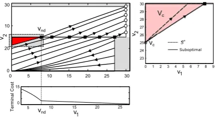
Proof The synthesis is more involved for this sequence. The terminal cost for the first
Neuron 2 spike is the value function from (30) withv2=0, that is,
ϕv1(τ1)
=V(v)|v2=0, (58)
which is a decreasing function inv1, andϕ(v1(τ1))is not differentiable with respect
tov1for somev1=vnd wherevnd∈ [0, VG](as shown in the bottom left of Fig.5).
Note that for any initial condition at the origin or on thev1 axis to the left of the
separatrix, OFF-BANG cannot lead to optimality, and for those cases, the extremals will be generated byu∗(t )=U for allt∈ [0, τ1]. Also, to the right of the separatrix
OFF-BANG will be the optimal policy as it is the only viable option in the presence of state constraints. So we can conclude that if there is indeed a switching to the left of the separatrix, then there must existvs ∈(0, VG]such that for v(0)= {(v1, v2):
v1=0, v2∈(vs, VG)}, the optimal policy will be OFF-BANG, whereas for v(0)=
{(v1, v2):v1=0, v2∈ [0, vs]}, the optimal control is BANG. Now we will calculate
this voltagevs, which acts as an onset for the change in optimal policy. Considering
the switching att= ˆt, we havev2(t )ˆ =vs and
Φ(t )ˆ =λ1(t )bˆ 1+λ2(t )bˆ 2=0. (59)
Since the Hamiltonian vanishes identically for our problem, we get
H(t )ˆ =1−a2vsλ2(t )ˆ =0. (60)
Also, from the transversality condition withλ0=1 we have
λ1(τ1)=
∂ϕ(v1(τ1))
∂v1
which is known. Since we reach the thresholdVT fromvs using the BANG control,
from (26) we have
τ1− ˆt=
1
a2
log
v
s−ba2
2U
VT −ba22U
. (62)
Using the fact that the adjoint variables satisfy linear homogeneous differential equa-tions, we can write
λ1(t )ˆ =
∂ϕ(v1(τ1))
∂v1
v
s−ba2
2U
VT −ba22U
−a1 a2
. (63)
From (59)–(63) we can solve forvs with
1+a2vsb1
b2
∂ϕ(v1(τ1))
∂v1
v
s−ba22U
VT −ba2
2U
−a1 a2
=0. (64)
If such vs exists, then the construction may be much more complicated with the
possible presence of a “cut-locus” type phenomenon, and we leave a detailed analysis of such a problem for future work. In our case, the terminal cost decreases with a rapid rate forv1∈ [0, vnd]and abruptly changes to a much smaller slope forv1∈(vnd, VG]
(see Fig.5) due to the nature of the value functions on either side of separatrixV−,
V+in (31) and (32). This results in a field of extremals trying to converge to the point
vnd, even when the monotonicity of the value function is not affected by the loss of
differentiability (see top left in Fig.5). We calculate the set of initial conditions for which this point can be attained, specifically vc= {(v1, v2):v1=0, v2∈ [vc, VG]},
wherevcdenotes the highest point onv2axis from which[VT vnd]T can be reached
via BANG control. This voltagevc and the set vc are shown in the right panel of
Fig.5. Now, the optimal control problem for v(0)∈vcsimply reduces to min J(u)=
τ1
0
dt
s.t. u(t )∈U
(65)
with the terminal constraint v(τ1)= [vnd VT]T and state constraints v1(t )≤VG,
v2(t )≤VT. This is similar to the selective spiking problem of Neuron 1, and indeed
the best control is a combination of BANG and boundary control as in (17),
u∗=
U fort≤tcwherev2(tc)=VT,
uarc fortc< t≤τ1wherev1(τ1)=vnd.
(66)
But this implies that Neuron 2 maintains the voltage(VT), even after the spike is
emitted, which violates our assumption that the neurons are reset instantaneously af-ter reachingVT, as described in (4). So the synthesisS∗ corresponding to (66) is
Fig. 5 A possible suboptimal synthesis is shown for the sequenceΣS= [2,1]. Note that the value
func-tion for the last spike, i.e. Neuron 1, plotted in the bottom panel, is not differentiable with respect tov1.
This is added as the terminal cost for the optimum control problem for the first spike in Neuron 2. In the right panel, the actual optimal solution and a constant control suboptimal synthesis proposed in (67) is shown.
minimum revolution [34], where the Goldschmidt extremal cannot be attained be-cause of the C1assumption on the extremals. Thus, any synthesisS for (65) will be suboptimal toS∗. For simplicity, we have picked a synthesis such that
usub=u
v(0) fort∈ [0, τ1], (67)
that is, a constant control that varies depending on the initial condition shown in Fig.5. For the set of initial conditions
v(0)= (v1, v2):v1=0,0≤v2< vc
∪ (v1, v2):0≤v1< VG, v2=0
, (68)
the optimal synthesis remains the same as the solution of P1 for Neuron 2.
4.2 Greedy Designs for Sequences with Arbitrary Length
From our analysis of the 2-spike sequences in the previous section, we can design the time optimal control for anyΣS ofMspikes (M≥2) without the subsequence
[2,1]. In addition, if we assume thata2< a1, then it can be shown using an inductive
argument that the overall synthesis can be constructed from the solutions of individual selective spiking problems in Propositions1and2.
In general, for aΣS with the subsequence[2,1], to illustrate the complexities of
sequence control, it is instructive to consider the 4-spike sequenceΣS= [1,2,1,1].
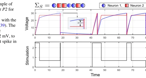
Fig. 6 Simulation example of the greedy algorithm for P2 for a target sequence
ΣS= [1,2,2,1,1,2,1]with the
nominal parameters in (39). The inset shows the synaptic contributionv2(t )=2 mV, to
Neuron 2 due to the first spike in Neuron 1.
Thus, we argue that, from a design perspective, a simple greedy approach, where we minimize the time for each spike inΣS progressively, constitutes an acceptable
and tractable approximation.
In Fig.6, we show the solution of the greedy controller for an arbitrary spike sequenceΣS.
4.2.1 Decoupling the Network for Longer Sequences
In applying the greedy approach, it is important to note that the synaptic contribution from the spiking neuron can carry the voltage of the other neuron in the network over the synaptic guardVG. Thus, we cannot readily apply the solution of P1 for the
following spike in the sequence (pattern), as the initial condition may violate the state constraint in (8) for P1. Here, we propose strategies to eventually utilize Propositions 1and2for the greedy design.
1. First, if the initial condition after any spike in the sequence (pattern), att=τ1, is
not within the relevant state spaceG, then we can applyu=0 untilt=t,t> τ1,
such that v(t)∈G. Then, we can apply the solution of P1 to induce the target spike.
2. Alternatively, we can modify the guardVG of the nontarget neuron at each step
of the greedy design, depending on the number of consecutive spikes in the target neuron in the sequence (pattern); for example, ifΣS= [1,1,2,2,2], then we can
set the guard voltage for Neuron 2 atVG(σ1) < VT −2ρ¯synfor the first spike and
VG(σ2) < VT− ¯ρsynfor the second spike. Thus, the relevant state space for the first
and second spikes will be modified toG(σ1)= [0, VT] × [0, VG(σ1)]andG(σ2)=
[0, VT] × [0, VG(σ2)], respectively. This ensures that whatever the contribution
is from the presynaptic neuron (in this case, Neuron 1), we start in the relevant state space for the next spike in the sequence (pattern). Once the target neuron changes toσ3=2, the guard voltage for Neuron 1 is determined by the number of
consecutive spikes in Neuron 2 (3 in this example), that is,VG(σ3) < VT −3ρ¯syn
and so on. Note that by successively reducing the guard voltage, the selective spiking problem may become infeasible as discussed in Sect.3.3.
In our examples of sequence and pattern control, we have used the first approach in developing the greedy design (see Figs.6and7).
5 Fixed-Time Selective Spiking and Spike Patterns
We now move to the problem of controlling timed spike patterns, that is, P3. It is intuitive that a basic necessary condition in this case is that the desired spike time exceeds the minimum selective spiking time, that is, the solution to P1.
Specifically, suppose that we want to achieve the target patternΣP= [(1, t1)], that
is, a spike in Neuron 1 at timet1. The cost function in P3 (14) reduces to J(u)=
t1−
τ1
0
dt
2
(69)
(subject to the selectivity constraint in (7)). Here,τ1denotes the achieved spike time,
andτ¯1 is the solution of P1 for an arbitrary initial condition v(0). Ifτ¯1≥t1, then
evidently that is our best option, and the solutions of (69) and P1 are the same, that is,τ1= ¯τ1.
For the other case,τ¯1< t1, contingent on controllability, a control must exist such
thatτ1=t1. If such a condition is met, then in general there may be multiple solutions
to the pattern control problem.
Herein, we consider one simple strategy involving the introduction of an off time ˆ
tto the optimal control solution of P1 such that
ˆ
t+τ1r=t1, (70)
whereτ1r is the solution of the time optimal control P1, for the initial condition v(t )ˆ. We noted earlier that the initial conditions for the selective spiking problem nomi-nally lie on either thev1orv2axis, under the assumption that one of the neurons has
just produced a spike. In this case, feasibility of (70) reduces to understanding those initial conditions that generate specific values ofτ1r.
5.1 Off-Time Insertion for Pattern Control
We characterize the relationship betweenτ1r and initial conditions via the notion of a
Λ-controllable set.
Definition 3 (Λ-Controllable set) Without loss of generality, theΛ-controllable set
ζ (Λ)of Neuron 1 is the set of initial conditions from which the selective spiking of Neuron 1 in P1 is achieved in timeΛ, that is,
ζ1(Λ)= (v1, v2):v(0)= [v1v2]T,t < Λs.t.v1(t )=VT, v2(t )≤VG
. (71)
TheΛ-controllable sets for system (11) are provided in AppendixA.4. Since we are interested in initial conditions along thev1andv2axes, we consider the functions
ω1:Λ→v1, such that(v1,0)∈ζ1(Λ),
ω2:Λ→v2, such that(0, v2)∈ζ1(Λ),
that is, the intersection of theΛ-controllable sets with the axes.
Earlier, we noted that the value function for the selective spiking of both neurons remains continuous on both thev1 andv2axes (i.e., from (36) and (44)). This fact,
together with the derivation of theΛ-controllable sets in the Appendix, allows us to conclude that the functions (72) are continuous inΛ.
Thus, we are able to ensure the existence of the off-time pattern control from (70), that is,
up=
0 fort∈ [0,tˆ], u∗ fort∈(t , tˆ 1],
(73)
whereu∗ comes from Proposition1or 2. The computation of the off-time tˆis ob-tained directly from theΛ-controllable sets and is provided in AppendixA.5. Thus, an overall pattern control strategy can be formulated as
Π∗=
u∗ ifτ¯1≥t1,
up ifτ¯1< t1.
(74)
5.2 Greedy Designs for Control of Long Patterns
We now consider the synthesis and design of the general pattern control problem P3. To begin, we consider the dynamic programming strategy studied in (51) but for P3. It turns out that the same issues pertaining to nondifferentiability of the value function in P2 persist in this case.
To illustrate this, consider the 2-spike target patternΣP = [(1, t1), (1, t2)]. Starting
from the last spikeσ2=1, we solve J(u)=
(t2−t1)−
τ2
τ1
dt
2
(75)
with the terminal and state constraints and use the value function of (75) as the ter-minal cost to the following optimal control problem:
J(u)=
t1−
τ1
0
dt
2
+ϕv2(τ1)
. (76)
Let us denote the solution of P1 for the second spike from the initial condition
v(0)= [0v2]T byτ¯. Then, depending onv2, the terminal cost in (76) takes the
fol-lowing form:
ϕ(v2)=
0 forv2s.t.τ¯≤(t2−t1),
((t2−t1)− ¯τ )2 forv2s.t.τ > (t¯ 2−t1).
(77)
Fig. 7 Simulation example of the greedy algorithm discussed in Sect.5.2for P3 for a target pattern ΣP = [(1,20), (2,30), (2,70), (1,95), (1,115), (2,120), (1,130)]with the nominal parameters in (39).
Similar to Fig.6, we show the synaptic contributionv2(t )=2 mV, to Neuron 2. We also explicitly
indicate the off-time(u=0)after the first (inset) and fourth spike in Neuron 1, as part of the decoupling strategy discussed in Sect.4.2.1.
5.3 Performance of Greedy Design Under Disturbance and Noise
In this section, we analyze the robustness of the greedy design when the coupled LIF network in (3) is subjected to noise and disturbances. Here we consider two types of uncertainties:
1. Incoming synaptic contributions of the pulse coupled form discussed in Sect.2.2.2, from other neurons
2. Noise in the dynamics of the membrane voltage of the neurons in (3) (process noise) and in measurement of these voltages (measurement noise). Note that in implementing the greedy controller in (74), we repeatedly apply Propositions1 and2, which are feedback control, that is, measurement is implicit.
In Fig.8(A), we show one realization of the voltage and control waveforms ford=
150 incoming spikes over the control horizon for the sameΣP used in the example
of Fig. 6. To illustrate the effect of these disturbances on the control strategy, in Fig.8(D), we plot the average Victor–Purpura (VP) distance [36,37] between the achieved and target spike trains as we vary the number of incoming spikesd over 50 trials. In each trial, we randomly select the arrival times of the spikes, the contribution and target of the synapse between the two neuron indices. The VP metric is a measure of synchrony between two spike patterns that involves three basic operations: adding or deleting any spike with cost 1, moving any spike with costq per unit time, and renaming any index of the spike with costk. Here, a lower VP distance corresponds to better control performance. We observe that with higher disturbance, represented by
d, the controller performs reasonably well with gradual degradation in the achieved patterns.
Next, we consider additive Gaussian noise both during the evolution of the mem-brane voltage and in measurement. Thus the linear model in (11) is modified to
˙
v(t )=Av(t )+bu(t )+w(t ),
Fig. 8 Induced voltage waveforms in the two neurons for ΣP = [(1,20), (2,30),
(2,70), (1,95), (1,115), (2,120), (1,130)] using the greedy design and the control under incom-ing synapses (A) and process, measurement noise ((B) for higher variance and (C) for lower variance). (D) Performance analysis of the controller in terms of VP distance with parametersq=1,k=1.5 against number of incoming spikesdas measure of disturbance. (E) Surface plot fitted to the simulation data of average VP distance (sameq,k) vs the process and measurement noise variances, in the course of solving the pattern control problem forΣP over different trials.
where the measurement vector y is a linear readout of the neuron voltages through a randomly selected matrix C, which is full rank, w(t ) and z(t ) follow multivari-ate Gaussian distributions with w(t )∼N(0, W )and v(t )∼N(0, Z), andW andZ
are the constant covariance matrices of the forms W =η12Iand Z=η22I, Iis the 2-dimensional identity matrix. Here, we compute the voltage estimates of the two neurons at each time step by means of a Kalman filter [38] and employ the feedback strategy in (74) based on these estimates. In Fig.8(B), (C), we plot the pattern control solutions for the sameΣP used in the example of Fig.6for smaller(η1=0.1, η2=1)
and higher(η1=1, η2=10)process and measurement variance. We observe that
controller’s ability to induce the target spike train is not compromised substantially, although with higher levels of noise, spurious spikes are generated, as indicated in panel (C). However, the noisy dynamics in (78) can result in a high frequency of switching in the control ((B), (C), bottom panel), especially during the boundary arc, that is, the nontarget neuron is to be held at guardVG. Panel (E) shows the
perfor-mance of the greedy design with respect to the average VP distance betweenΣP and
achieved patterns over 50 different trials, as we change the level of noise during the evolution and measurement phase.
![Fig. 4 Optimal Synthesis for Sequencesdifferentiable. The optimal trajectories from several initial conditions are shown.thesis forfor sequenceparameters ( [1,1], [1,2] and [2,2] is shown in (a) (b) (c) for the nominal39)](https://thumb-us.123doks.com/thumbv2/123dok_us/913508.1589181/18.439.56.388.52.169/optimal-synthesis-sequencesdifferentiable-optimal-trajectories-conditions-sequenceparameters-nominal.webp)
![Fig. 7 Simulation example of the greedy algorithm discussed in Sect.Similar to Fig.Σ 5.2 for P3 for a target patternP = [(1,20),(2,30),(2,70),(1,95),(1,115),(2,120),(1,130)] with the nominal parameters in (39)](https://thumb-us.123doks.com/thumbv2/123dok_us/913508.1589181/26.439.113.330.51.186/simulation-example-algorithm-discussed-similar-patternp-nominal-parameters.webp)