DOI 10.1186/s13408-016-0039-8
R E S E A R C H Open Access
Ill-Posed Point Neuron Models
Bjørn Fredrik Nielsen1·John Wyller1
Received: 17 November 2015 / Accepted: 20 April 2016 /
© 2016 Nielsen and Wyller. This article is distributed under the terms of the Creative Commons Attribution 4.0 International License (http://creativecommons.org/licenses/by/4.0/), which permits unrestricted use, distribution, and reproduction in any medium, provided you give appropriate credit to the original author(s) and the source, provide a link to the Creative Commons license, and indicate if changes were made.
Abstract We show that point-neuron models with a Heaviside firing rate function can be ill posed. More specifically, the initial-condition-to-solution map might be-come discontinuous in finite time. Consequently, if finite precision arithmetic is used, then it is virtually impossible to guarantee the accurate numerical solution of such models. If a smooth firing rate function is employed, then standard ODE theory im-plies that point-neuron models are well posed. Nevertheless, in the steep firing rate regime, the problem may become close to ill posed, and the error amplification, in finite time, can be very large. This observation is illuminated by numerical exper-iments. We conclude that, if a steep firing rate function is employed, then minor round-off errors can have a devastating effect on simulations, unless proper error-control schemes are used.
Keywords Point-neuron models·Ill posed·Numerical solution
1 Introduction
Modeling of electrical potentials has a long tradition in computational neuroscience. One model with some physiological significance is the voltage-based system
τu(t )= −u(t )+ωSβ
u(t )−uθ+q(t ), t∈(0, T], (1)
u(0)=u0, (2)
where
u(t ),q(t )∈RN, t∈(0, T],
B
B.F. Nielsen1 Department of Mathematical Sciences and Technology, Norwegian University of Life Sciences,
uθ,u0∈RN, ω∈RN×N,
τ∈RN×Nis diagonal,
S(x)=1 2
1+tanh(x),
Sβ[x] =S(βx),
Sβ[x] =
Sβ[x1], . . . , Sβ[xN]
T
, x=(x1, . . . , xN)T ∈RN.
In the rate model (1)–(2), each component functionui(t )of u(t )represents the time dependent potential of theith unit in a network ofN units. The nonlinear function Sβ is called the firing rate function,{ωij}are the connectivities, and q(t )models the external drive. A detailed derivation of this model can be found in [1–3].
The purpose of this paper is to explore the properties of the
initial-condition-to-solution map
Rβ:u0→u(T ), T <∞, (3) associated with (1)–(2). Note that we use the subscriptβ to emphasize thatRβ de-pends on the steepness parameterβ, and thatR∞corresponds to using a Heaviside firing rate function, i.e.S∞=H. We will also make use of the standard notation
f∞= sup 1≤i≤N
|fi|, f=(f1, . . . , fN), (4)
for the supremum norm throughout this paper.
A simple example, presented in Sect.4, shows thatR∞can become discontinu-ous. Hence, the model is mathematically ill posed [4,5] and round-off errors of any size can corrupt computations. We conclude that it is very difficult to produce reli-able simulations with such models. Since all norms for finite dimensional spaces are equivalent, it is not possible to “circumvent” this problem by changing the involved topologies.
According to standard ODE theory (AppendixA),Rβ, withβ <∞, is continuous, but the size of the error-amplification ratio
E(T;β)=u(T;β)− ˜u(T;β)∞
u0− ˜u0∞ (5)
know, results which explicitly discuss the ill-posed nature of (1)–(2) whenβ= ∞, and how this property yields extra numerical challenges in the steep, but smooth, firing rate regime, has not previously been published.
Remark We would like to point-out the following: Assume that an initial condition is
close to an unstable equilibrium. Our results should not be interpreted as expressing the mundane fact that a perturbation of this initial condition, moving it to another region with completely different dynamical properties, may lead to large changes in the solution. In fact, we show that the error-amplification ratio can be huge, during small time intervals, even though the perturbation does not change which neurons are active. That is, the change in the initial condition is not such that it changes the qualitative behavior of the dynamical system for 0< t1—only the quantitative properties are dramatically altered. This can happen in the steep firing rate regime.
2 Numerical Results
Let us first compute the error-amplification ratio (5) for some simple problems.
Example 1 Consider the following model of a single point neuron, i.e.N=1,
u(t )= −u(t )+0.9Sβ
u(t )−0.6+0.151, t∈(0, T],
u(0)=u0=0.6.
We used Matlab’sode45solver, with the default error-control settings andT =0.1, to compute numerical approximations of
u(t )=u(t;β) forβ=1, . . . ,200.
Also a second series of simulations were performed, using the same selection of values for the steepness parameter, but with the perturbed initial condition
˜
u0=u0−10−5. (6) The corresponding solution is denotedu(t )˜ = ˜u(t;β).
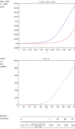
Plots ofuandu˜, withβ=200, are displayed in Fig.1. Note that in both cases the neuron fires, i.e. the change in the initial condition is not such that it has moved from one side of an unstable equilibrium to the other side. Even so, according to Fig.2and Table1, the error-amplification ratioE(T;β), due to the minor perturbation (6) of the initial condition, is in the range[80.6,1054.1]forβ∈ [100,200], and also very large forβ=50,75.
Simulations with the strict error-control setting
odeset(’RelTol’,1e-13,’AbsTol’,1e-13)
Fig. 1 Numerical results, with steepness parameterβ=200, for the problem studied in Example1
Fig. 2 Error-amplification ratio, withT=0.1, as a function of the steepness parameterβfor the problem studied in Example1
Table 1 Error-amplification ratio, withT=0.1, associated
with Example1 β 1 25 50 75
E(T;β)=|u(T;|uβ)− ˜u(T;β)|
0− ˜u0| 0.95 2.79 8.58 26.41
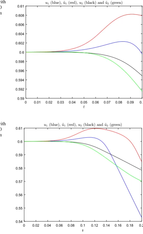
Example 2 Let us consider a model of two point neurons:
u1(t )= −u1(t )+0.9Sβu1(t )−0.6+1.0Sβu2(t )−0.6−0.3492, t∈(0, T], u2(t )= −u2(t )−0.1Sβ
u1(t )−0.6
+0.6Sβ
u2(t )−0.6
+0.3501, t∈(0, T], u1(0)=u1,0=0.6,
Fig. 3 Numerical results, with steepness parameterβ=200 andT=0.1, for the problem studied in Example2
Fig. 4 Numerical results, with steepness parameterβ=150 andT=0.2, for the problem studied in Example2
The same procedure as in Example1was used, but with the perturbed initial condition
˜
u1(0)= ˜u1,0=u1,0−10−5, ˜
u2(0)= ˜u2,0=u2,0+10−5.
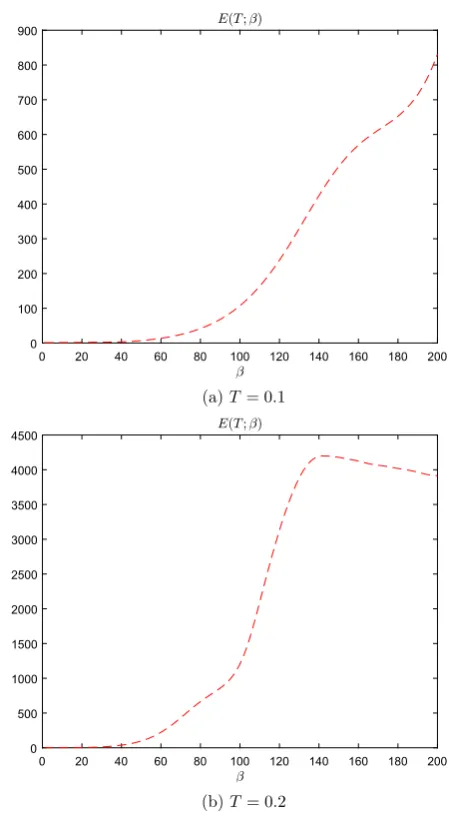
Fig. 5 Error-amplification ratio as a function of the steepness parameterβfor the problem studied in Example2
As in Example 1, we used Matlab’s ode45 solver with the standard settings. Computations with the strict error-control parameters
odeset(’RelTol’,1e-13,’AbsTol’,[1e-13 1e-13]) (7)
produced virtually the same results. The simulations were also “confirmed” by our explicit Euler implementation with time-stept=10−7.
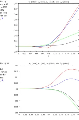
Figure6shows numerical results computed with Matlab’sode15ssolver, em-ploying the default error-control settings. The curves shown in this figure are very different from the graphs displayed in Fig.4, which were computed by theode45
Fig. 6 Results generated by Matlab’sode15ssolver, with steepness parameterβ=150 andT=0.2. Note that the
curves are very different from
the graphs produced with the
ode45solver; see Fig.4
Fig. 7 Results generated by an explicit Euler scheme: t=0.01,β=150, and T =0.2. Note that the curves are rather different from the graphs produced with the
ode45solver; see Fig.4
trivial to solve (with the strict error-control setting (7), ode15salso managed to produce the curves shown in Fig.4).
Ifu1(t )≈uθ andu2(t )≈uθ, then
u1(t ),u2(t )≤2uθ=2·0.6=1.2,
and the model implies that
u1(t )≤1.2+0.9+1.0+0.3492=3.4492,
u2(t )≤1.2+0.1+0.6+0.3501=2.2501,
that this is not the case. (In computational mathematics it is well known that the accu-racy of the finite difference approximation[u1(t+t )−u1(t )]/t, of the derivative u1(t ), depends on the second order derivativeu1(t ), which in our case is of order O(β). This explains the poor approximation obtained with time-stept=0.01.)
3 Analysis
The purpose of this section is to present an analysis of the error-amplification ratio (5) and thereby explain the main features of our numerical results. Even though the Picard–Lindelöf theorem [9,10] asserts that (1)–(2) has a unique solution u(t ), pro-vided that q(t )is continuous and thatβ <∞, it is virtually impossible to determine a simple expression for u(t ). On the other hand, if u(t )≈uθ andβ <∞, then we can linearizeSβ to get an approximate model, which is much easier to work with.
3.1 Linearization
The linearization ofSβ about zero reads
Lβ(x)=Sβ[0] +Sβ[0]x
=1 2+
1
2βx. (8)
Defineτ=I, the identity matrix, then the linear approximation of (1)–(2) reads s(t )= −s(t )+ωLβs(t )−uθ+q(t )
= −s(t )+ω
1 21+
1 2β
s(t )−uθ +q(t )
=
1 2βω−I
s(t )+1
2ω(1−βuθ)+q(t )
=As(t )+d+q(t ), (9)
s(0)=u0, (10)
where
A=A(β)=1
2βω−I, (11)
d=d(β)=1
2ω(1−βuθ).
The linearized problem with a perturbed initial condition becomes
˜
s(t )=A˜s(t )+d+q(t ), ˜
and the difference s(t )− ˜s(t )obeys
s(t )− ˜s(t )=As(t )− ˜s(t ), s(0)− ˜s(0)=u0− ˜u0. Therefore,
s(t )− ˜s(t )=(u0− ˜u0)eAt, and the error-amplification ratio can be written in the form
s(T )− ˜s(T )∞ u0− ˜u0∞ =
(u0− ˜u0)eAT∞
u0− ˜u0∞ . (12)
Since the entries of A=A(β)are of orderO(β), see (11), we conclude that the error-amplification ratio for the linearized model is of exponential orderO(eβ). Is this also the case for the highly nonlinear model (1)–(2)? We will now explore this issue, but first we would like to make a short remark.
Remark Recall the definition (8) ofLβ. If we replaceSβ in (1)–(2) with
˜ Lβ(x)=
⎧ ⎪ ⎨ ⎪ ⎩
1, x > 1β, Lβ(x), x∈ [−β1,1β], 0, x <−β1,
then the analysis of the linearized model, presented above, would also be valid for (1)–(2), provided that
s(t )−uθ∞,˜s(t )−uθ∞∈
0,1 β
, t∈ [0, T].
Similarly to the sigmoid functionSβ,L˜β also converges point-wise to the Heaviside function asβ→ ∞. If one employs the sigmoid function in the point-neuron model, then the analysis, as we will see below, becomes much more involved.
3.2 Preparations
Letβmax,Tˆ, andαbe arbitrary positive constants. It is easy to construct a smooth vector-valued function z satisfying
z(t )−uθ∞∈
0, 0.9 βmax1+α
, t∈ [0,Tˆ]. (13)
Hence, defining the source as
q(t )=τz(t )+z(t )−ωSβmaxz(t )−uθ, t∈(0,Tˆ],
u(t;β)of (1)–(2) depends continuously on 0< β <∞; see AppendixB. Conse-quently, there existsβmin¯ < βmaxsuch that
u(t;β)−uθ∞∈
0, 1 βmax1+α
, t∈ [0,Tˆ], β∈ [ ¯βmin, βmax].
For the sake of simple notation, we will in our analysis write u, or u(t ), instead of u(t;β).
Furthermore, according to the analysis presented in AppendicesA–C,udepends continuously on both the initial condition u0 and the steepness parameterβ, when 0< β <∞. Motivated by this property of (1)–(2), we assume that both u and u,˜ whereu denotes the solution of (˜ 1) generated by a perturbed initial conditionu(˜ 0)= ˜
u0, satisfy
u(t )−uθ
∞,u(t )˜ −uθ∞∈
0, 1 βmax1+α
, t∈ [0,Tˆ], β∈ [ ˆβmin, βmax], (14)
whereβˆmin< βmax. Then, by invoking the triangle inequality, we find that
u(t )− ˜u(t )
∞≤
2
βmax1+α
, t∈ [0,Tˆ], β∈ [ ˆβmin, βmax], (15) which will be small ifβmax is large. Even so, as will become evident below, the error-amplification ratio (5) can be significant and lead to erroneous results.
Let s ands denote the associated solutions of the linearized model (˜ 9)–(10). From (14) we find that the initial conditions u0andu0˜ satisfy
u0−uθ∞,˜u0−uθ∞∈
0, 1 βmax1+α
.
Since s and˜s are continuous with respect tot, the same initial conditions are em-ployed in the linearized model, and these solutions depend continuously on 0< β < ∞, it follows that there existT >˜ 0 andβmin˜ < βmaxsuch that
s(t )−uθ∞,˜s(t )−uθ∞∈
0, 1 βmax1+α
, t∈ [0,T˜], β∈ [ ˜βmin, βmax]. (16) The main point of this discussion is to show that there exist (smooth) source terms q and perturbations of the initial condition such that (14) holds, regardless how large
ˆ
T , βmax, α >0 are. Also, the solutions of the linearized model will satisfy (16). For the sake of simple notation, letT =min{ ˜T ,Tˆ}andβmin=max{ ˜βmin,βˆmin}.
The triangle inequality implies that
e(t )=u(t )−s(t ), ˜
e(t )= ˜u(t )− ˜s(t ) obey
e(t )
∞,e(t )˜ ∞∈
0, 2 βmax1+α
We will derive a bound fore(T )∞. The analysis of˜e(T )∞is completely analo-gous, and thus it is omitted.
3.3 Linearization Error
Subtracting (9) from (1), and keeping in mind that we consider the caseτ=I, yields ei(t )= −ei(t )+
j ωi,j Sβ
uj(t )−uθ
−Lβ
sj(t )−uθ
,
i=1,2, . . . , N, where we use the notation e(t )= [e1(t ), e2(t ), . . . , eN(t )]T, and sim-ilarly for the entries of u(t )and s(t ). Integrating and invoking the fact thatei(0)=0, we get
ei(T )= −
T
0
ei(t ) dt+
T
0
j
ωi,jSβuj(t )−uθ−Lβsj(t )−uθdt, (18)
i=1,2, . . . , N.
The triangle inequality, Taylor’s theorem and Eq. (8) forLβimply that
Sβ
uj(t )−uθ
−Lβ
sj(t )−uθ≤Sβ
uj(t )−uθ
−Lβ
uj(t )−uθ +Lβ
uj(t )−uθ
−Lβ
sj(t )−uθ
≤β21 2maxy S
(y)uj(t )−uθ2
+1
2βej(t ) ≤β2β−2−2α
+1
2βej(t )
≤β−2α+1
2βej(t ),
where the second last inequality follows from (14). By combining this with (18), and the triangle inequality, one finds that
ei(T )≤
T
0
ei(t )dt+BT β−2α+ 1 2βB
T
0
e(t )∞dt
≤
T
0
1+1 2Bβ
e(t )∞dt+BT β−2α, where
B=max i
Since this must hold fori=1,2, . . . , N,
e(T )
∞≤
T
0
1+1 2Bβ
e(t )∞dt+BT β−2α, and Grönwall’s inequality implies that
e(T )∞≤BT β−2αexp
1+1 2Bβ
T
. (19)
3.4 Error-Amplification Ratio Clearly,
u− ˜u=u−s+s− ˜s+ ˜s− ˜u
=e+s− ˜s− ˜e, (20)
and the reverse triangle inequality yields
u− ˜u∞≥s− ˜s∞− e− ˜e∞. From (12) it follows that the error-amplification ratio (5) satisfies
E(T;β)= u(T;β)− ˜u(T;β)∞ u0− ˜u0∞
≥(u0− ˜u0)eAT∞ u0− ˜u0∞
I=I (T;β)
−e(T )− ˜e(T )∞ u0− ˜u0∞
II=II(T;β)
.
Recall that the entries of the matrixA=A(β)are of orderβ; see (11). To derive a bound for II(T;β), we employ (19), and a similar inequality for˜e(T )∞,
e(T )− ˜e(T )∞ u0− ˜u0∞ ≤
2BT β−2αexp[(1+12Bβ)T] u0− ˜u0∞
=β−2α 2BT u0− ˜u0∞exp
1+1 2Bβ
T
.
Hence, if
2BT
u0− ˜u0∞ (21)
is not very large, β is fairly large and, e.g., α≥0.5, then the size of the error-amplification ratioE(T;β)is dominated byI (T;β), i.e. by the term stemming from the linearized model. (Note that (20) and the reverse triangle inequality also imply that|E(T;β)−I (T;β)| ≤II(T;β).)
In our numerical experiments,u0− ˜u0∞=10−5andβmax=200. That is,u0− ˜
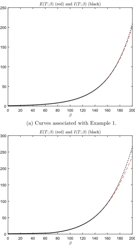
Fig. 8 Error-amplification ratio E(T;β), red dashed lines, as a function of the steepness parameterβ. The black dotted
curves are the graphs of
I (T;β). These plots were generated withT =0.06
It is virtually impossible to distinguish between the curves ofE(T;β)andI (T;β), β=1,2, . . . ,200, whenT =10−4 (curves not presented). Figure 8illustrates that I (T;β)also yields a reasonable approximation ofE(T;β)forT =0.06.
Fig.4an initial perturbation of size 10−5 is increased to an error of approximately 0.04=4 %.
Remark Assume that the·∞-norm of the source term q(t )is bounded. Then, since 0< Sβ[x]<1 for allx∈R, it follows from (1) that bothu(t )∞and˜u(t )∞are bounded independently of the size of the steepness parameterβ, at least when u(t )≈ uθ andu(t )˜ ≈uθ. Consequently, also the differenceu(T )− ˜u(T )∞ is bounded independently ofβ >0. Our results therefore might appear to be somewhat counter-intuitive: But note that we have only argued that the error-amplification ratio (5) may, approximately, be of orderO(eβ). Ifβis large, this can cause severe numerical challenges.
We would also like to comment that standard theory for general dynamical systems
z(t )=Ft,z(t ), t∈(0, T], z(0)=z0,
relies on the size ofF, which for the point-neuron model (1)–(2) is of orderO(β). Also, F(t,z)= −z+ωSβ[z−uθ] +q(t )is not Lipschitz continuous with respect to z whenβ= ∞, which the Picard–Lindelöf theorem [9,10] requires. (F is not even continuous whenβ= ∞.)
The maximum error bound (15), valid when u−uθ andu˜−uθ satisfy (14), sug-gests that setting β= ∞ might provide a solution to the issues discussed above. Unfortunately, as will be explained in the next section, this is not the case.
4 Ill Posed
We will now show that (1)–(2) can become truly ill posed, if a Heaviside firing rate function is employed. More specifically, the initial-condition-to-solution map, in fi-nite time, can be discontinuous.
Consider the caseN=1,τ=1 and no source term:
v(t )= −v(t )+ωHv(t )−uθ
,
v(0)=u0.
(22)
If, for 0< 1,
u0=uθ+ > uθ and u0=uθ− < uθ, then
v(t )=ω+(uθ+−ω)e−t,
v(t )=(uθ−)e−t,
provided thatω > uθ. Consequently,
R∞(u0)−R∞(u0)=v(T )−v(T )=ω
whereR∞ denotes the initial-condition-to-solution map (3). We conclude that, no matter how closeu0andu0are, the differencev(T )−v(T )between the correspond-ing solutions will not become small. Hence,R∞ is discontinuous. It follows that the initial value problem, with a Heaviside firing rate function, is ill posed, in finite time—at least in the sense of Hadamard. Also note that, unlessω=2uθ,uθ is not a stationary solution of (22), i.e. not an unstable equilibrium.
The error-amplification ratio for this ill-posed problem becomes infinite when →0:
|v(T )−v(T )| |u0−u0| =
|R∞(u0)−R∞(u0)| |u0−u0|
=|ω(1−e−T)+2e−T| 2
>ω(1−e
−T)
2 → ∞
as→0, for anyT >0.
One may consider this issue from a more pragmatic point of view. Letvt denote a numerical approximation ofv. If a Heaviside firing rate function is employed, then H (vt −uθ)must be evaluated in some line of the simulation software. This is an unstable procedure becauseH has a jump discontinuity at 0, and round-off errors of any size can corrupt computations.
In contrast to this, provided thatβ <∞,
u(T )− ˜u(T )∞≤ u0− ˜u0∞·exp(A+βB)T, (23)
see the analysis of the model (1)–(2) presented in AppendixA. Here,u0˜ is any per-turbation of the initial condition u0, andAandBare positive constants depending on the matricesτ andω, but not onβ. This inequality shows that the initial-condition-to-solution mapRβ,β <∞, also is continuous at unstable equilibria.
5 Conclusions and Discussion
SinceR∞can become discontinuous, it is virtually impossible to guarantee the accu-rate numerical solution of point-neuron models which employ a Heaviside firing accu-rate function: Any round-off errors can potentially corrupt simulations. Alternatively, one may stop the simulation as soon as the solution hits the jump discontinuity, i.e. the threshold value for firing.
threshold value for firing, might be capable of handling the numerical error amplifi-cation.
Let
Fβ;t1,t2:u(t1)→u(t2), t2> t1≥0,
be the operator which maps the solution of the point-neuron model (1)–(2) from time t1to timet2. Note that the action ofFβ;t1,t2 can be determined by solving the
point-neuron model with u(t1)as initial condition. Therefore, from the argument presented above, it follows that the error amplification ratio associated with Fβ;t1,t2 may be
large, provided thatβ 1. We conclude that the issues pointed out in this study cannot necessarily be avoided by using an initial condition which is far from the threshold value uθfor firing. In fact, it seems that one must prove that u(t )never gets close to uθ fort >0—a herculean task, if correct.
From a modeling perspective one might wonder: Should a voltage-based model of cortex be ill posed or “almost ill posed”? If so, then models employing a Heaviside firing rate function cannot be robustly solved with finite precision arithmetic and regularized approximations are numerically challenging [4,5].
We fear that similar unfortunate properties, to those discussed in this paper, might be valid for models which can be written in the form
z(t )=Fβt,z(t ), t∈(0, T], z(0)=z0,
whereFβ → ∞whenβ→ ∞. This can, e.g., be the case for a number of models in use in computational neuroscience and gene regulatory networks.
An easy solution to the issues raised in this paper, is to avoid steep firing rate functions. Ifβis fairly small, then standard ODE theory [9,10] and textbook mate-rial about their numerical treatment can be used, provided that the source term q(t ) is continuous. Nevertheless, steep sigmoid functions are popular in computational neuroscience.
Competing Interests
The authors declare that they have no competing interests.
Authors’ Contributions
All authors contributed equally to the writing of this paper. All authors read and approved the final manuscript.
Appendix A: Continuous Dependence on the Initial Condition
We will prove the stability estimate (23), which holds ifβ <∞. Let u andu denote˜ the solutions of (1) corresponding to the initial conditions u0andu0˜ , respectively. For the purpose of detailing the derivation of this estimate, we work with the components of these vector functions, i.e.,
u(t )=
⎛ ⎜ ⎜ ⎜ ⎝ u1(t ) u2(t ) .. . uN(t ) ⎞ ⎟ ⎟ ⎟
⎠, u(t )˜ = ⎛ ⎜ ⎜ ⎜ ⎝ ˜ u1(t ) ˜ u2(t ) .. . ˜ uN(t ) ⎞ ⎟ ⎟ ⎟ ⎠, u0= ⎛ ⎜ ⎜ ⎜ ⎝ u1,0 u2,0 .. . uN ,0 ⎞ ⎟ ⎟ ⎟
⎠, u0˜ =
⎛ ⎜ ⎜ ⎜ ⎝ ˜ u1,0 ˜ u2,0 .. . ˜ uN ,0 ⎞ ⎟ ⎟ ⎟ ⎠.
Let us also assume that the diagonal entries{τi}, of the diagonal matrixτ, are posi-tive, and let{ωij}denote the entries ofω.
We first observe that the component functionsui and ui˜ satisfy the fixed point problems
ui(T )=ui,0+τi−1
T
0
−ui(t )+ N
j=1
ωijSβuj(t )−uj,θ+qi(t ) dt,
˜
ui(T )= ˜ui,0+τi−1
T
0
− ˜ui(t )+ N
j=1
ωijSβuj˜ (t )−uj,θ+qi(t ) dt,
from which we find, by using the triangle inequality, that
ui(T )− ˜ui(T )≤ |ui,0− ˜ui,0| +τi−1
T
0
ui(t )− ˜ui(t )dt
+τi−1 N
j=1 |ωij|
T
0
Sβ
uj(t )−uj,θ
−Sβ
˜
uj(t )−uj,θdt.
Then, by exploiting the fact that
Sβ(x)−Sβ(y)≤ 1
2β|x−y|
for allx, y∈R, we get
ui(T )− ˜ui(T )≤ |ui,0− ˜ui,0|
+τi−1
T
0
+τi−11 2β
N
j=1 |ωij|
T
0
uj(t )− ˜uj(t )dt
≤ |ui,0− ˜ui,0|
+τi−1
!
1+1 2β
N
j=1 |ωij|
" T
0
u(t )− ˜u(t )∞dt,
where we in the final step have used the definition of the supremum norm (4). Thus, we arrive at the inequality
u(T )− ˜u(T )∞≤ u0− ˜u0∞
+ max 1≤i≤N
#
τi−1
!
1+1 2β
N
j=1 |ωij|
"$ T
0
u(t )− ˜u(t )∞dt.
The stability estimate (23), with
A= max 1≤i≤N
τi−1, B=1 21max≤i≤N
!
τi−1 N
j=1 |ωij|
"
,
then follows from Grönwall’s lemma.
Appendix B: Continuous Dependence on the Steepness Parameter
For the sake of completeness, we also show that the solution of the initial value prob-lem (1)–(2) depends continuously on the steepness parameter β. Letβ andβˆ be steepness parameters for the firing rate function. We fix the initial condition and the connectivity parameters of (1)–(2). The solutions corresponding toβ andβˆ are de-noted by u andu, respectively. We readily obtainˆ
ui(T )=ui,0+τi−1
T
0
−ui(t )+ N
j=1 ωijSβ
uj(t )−uj,θ
+qi(t ) dt,
ˆ
ui(T )=ui,0+τi−1
T
0
− ˆui(t )+ N
j=1 ωijSβˆ
ˆ
uj(t )−uj,θ
+qi(t ) dt,
for the component functionsui anduˆi of u andu, respectively. We now make use ofˆ the property
Sβ[uj−uj,θ] −Sβˆ[ ˆuj−uj,θ]≤ 1 2
β|uj− ˆuj| + |β− ˆβ|
|uj,θ| + | ˆuj|
for the firing rate function, and we get the chain of inequalities
ui(T )− ˆui(T )≤τi−1
T
0
ui(t )− ˆui(t )dt
+τi−1 N
j=1 |ωij|
T
0
Sβ
uj(t )−uj,θ
−Sβˆuˆj(t )−uj,θ dt
≤τi−1
T
0
ui(t )− ˆui(t )dt
+1 2βτ −1 i N
j=1 |ωij|
T
0
uj(t )− ˆuj(t )dt
+1
2|β− ˆβ|τ
−1 i
N
j=1 |ωij|
|uj,θ|T+
T
0
uˆj(t )dt
. (24)
Since 0≤S(x)≤1, we find the bound
uˆj(s)≤Cj(s), s∈ [0, T],
Ci(s)≡ N
j=1 |ωij| +
s
0
αi(s−t )qi(t ) dt
+
!
|ui,0| − N
j=1 |ωij|
"
τiαi(s)
= N
j=1 |ωij|
1−τiαi(s)
+
s
0
αi(s−t )qi(t ) dt
+ |ui,0|τiαi(s),
uniformly inβ, for the solutions of (1)–(2). Here,
αi(t )= 1 τi
e−t /τi,
and it follows that the integrals %0T| ˆuj(t )|dt in (24) can be bounded by β -independent constants. Thus, we end up with the bounding inequality
u(T )− ˆu(T )∞≤C(T )|β− ˆβ| +(A+βB)
T
0
u(t )− ˆu(t )∞dt,
whereAandBare as defined in AppendixAand
C(T )=1 2t∗∈[sup0,T]
max 1≤i≤N
τi−1 N
j=1 |ωij|
|uj,θ|t∗+
t∗
0
Cj(t ) dt .
Grönwall’s lemma yields the stability estimate
u(T )− ˆu(T )∞≤C(T )|β− ˆβ| ·exp(A+βB)T
q(T )
which proves that the solution of (1)–(2) depends continuously on the steepness pa-rameterβ <∞of the firing rate function.
Since q(T )is increasing, it is possible to extract further information from this argument. More specifically, let
U=
&
v(t )v(t )∈RN, t∈ [0, T]and sup t∈[0,T]
v(t ) ∞<∞
'
, (26)
with norm
vU= sup t∈[0,T]
v(t )
∞. (27)
Then we can conclude that the mapping
R+→U,
β→u(t;β), t∈ [0, T],
is continuous.
Appendix C: Continuous Dependence on the Initial Condition and the
Steepness Parameter
We finally prove that the solution u=u(t;u0, β)of (1)–(2) depends continuously on (u0, β). The proof of this fact proceeds as follows: By exploiting the triangle inequality and the stability estimates (23) and (25), we find that
u(T; ˜u0,β)ˆ −u(T;u0, β)∞
≤u(T; ˜u0,β)ˆ −u(T;u0,β)ˆ ∞+u(T;u0,β)ˆ −u(T;u0, β)∞ ≤˜u0−u0∞+C(T )| ˆβ−β| ·exp(A+βB)T
g(T )
and we are done. Here u0andu0˜ denote two initial conditions of (1), whileβˆandβ are two steepness parameters.
The functiong(T )is increasing, and we conclude that the mapping
RN×R
+→U,
(u0, β)→u(t;u0, β), t∈ [0, T], whereUis defined in (26)–(27), is continuous.
References
2. Ermentrout B. Neural networks as spatio-temporal pattern-forming systems. Rep Prog Phys. 1998;61:353–430.
3. Faugeras O, Veltz R, Grimbert F. Persistent neural states: stationary localized activity patterns in nonlinear continuousn-population,q-dimensional neural networks. Neural Comput. 2009;21:147– 87.
4. Engl HW, Hanke M, Neubauer A. Regularization of inverse problems. Dordrecht: Kluwer Academic; 1996.
5. Well-posed problem. Wikipedia.https://en.wikipedia.org/wiki/Well-posed_problem(2016). 6. Coombes S. Waves, bumps, and patterns in neural field theories. Biol Cybern. 2005;93:91–108. 7. Veltz R, Faugeras O. Local/global analysis of the stationary solutions of some neural field equations.
SIAM J Appl Dyn Syst. 2010;9:954–98.
8. Potthast R, beim Graben P. Existence and properties of solutions for neural field equations. Math Methods Appl Sci. 2010;33:935–49.
9. Hirsch MW, Smale S. Differential equations, dynamical systems and linear algebra. New York: Aca-demic Press; 1974.