https://doi.org/10.5194/ms-10-309-2019
© Author(s) 2019. This work is distributed under the Creative Commons Attribution 4.0 License.
Computer-aided synthesis of spherical and planar 4R
linkages for four specified orientations
Guangming Wang1, Hao Zhang1, Xiaoyu Li1, Jiabo Wang2, Xiaohui Zhang1, and Guoqiang Fan1
1College of Mechanical and Electronic Engineering, Shandong Agricultural University, Tai’an, China 2College of Engineering, Nanjing Agricultural University, Nanjing, China
Correspondence:Guangming Wang (gavinwang1986@163.com)
Received: 17 June 2018 – Revised: 25 February 2019 – Accepted: 23 May 2019 – Published: 25 June 2019
Abstract. According to the burmester theory, an infinite number of spherical or planar 4R linkages for a specific four-orientation task can be synthesized, but most of the linkage solutions calculated by this method are invalid because of motion defect, poor performance and others. In order to improve the synthesis efficiency, a program package based onMatlabis developed to find a satisfied linkage solution automatically and quickly. Firstly, the calculation on circle points and the center points based on the burmester theory in spherical problems is intro-duced. Secondly, the calculation methods of linkage defect discrimination, linkage type classification, linkage performance evaluation and solutions visualization based on the theory of spherical trigonometry are presented respectively. Thirdly, the synthesis calculation of program package is extended to the planar 4R linkage based on the theory of planar analytic geometry. Finally, the examples of the spherical synthesis problem and the planar synthesis problem based on solutions map are introduced to test the program package, the result proves this program package is effective and flexible.
1 Introduction
In this paper, the study work is to design a 4R linkage which can guide its coupler to pass four specified orientations smoothly and orderly. In order to accomplish this design task, graphing method and computer-aided synthesis method are used mainly at present. The theoretical basis of the graphing method is the theory ofburmester, that is to say, connecting any two groups of center points and their corresponding cir-cle points can obtain the desired linkage solution. Although the selection of center points or circle points are optional, majority of the linkage solutions have some problems such as circuit defect, branch defect, order defect or poor motion performance (Wang et al., 2010; Baskar and Bandyopadhyay, 2019a). For the linkage motion defect, the classical defect discrimination method is to study the segmentation technique of theburmestercurve (Filemon, 1972; Waldron and Strong, 1978; Gupta and Beloiu, 1998). Considering the inefficiency of the graphing method and the inaccuracy of the discrimi-nation of defective linkages, such as discarding some feasi-ble solutions as uncertain solutions, its application have some limitations. With the development of computer-aided design,
problems. The method oftype mapmaps all the linkage so-lutions obtained by computer into a two-dimensional coordi-nate system and marks different linkage types with different colors. At the same time, the defective linkage solutions can be hidden. The blindness of linkage synthesis can be reduced by using thetype mapbased on these synthesis software, but there are still some shortcomings: firstly, the biggest prob-lem is that it is not flexible enough and must be designed the linkage according to the process set by the software; sec-ondly, few software besidesSphinxhave the synthesis ability of spherical linkage; finally, thetype mapmethod can only express the solutions distribution with different linkage type in the solution domain, however, in practical synthesis prob-lems, the transmission performance and installation position of linkage solutions are more important than linkage types (Mendoza-Trejo et al., 2015). In order to make up for the shortcomings of the graphing method and computer-aided synthesis method mentioned above, a series of flexible func-tions for the synthesis, analysis and plotting of linkages are constructed under Matlab. These functions can be used for the synthesis calculation of spherical and planar 4R linkages. Compared with the previous studies, the main work of this study is as follows: the existing color-codedtype mapmethod is improved to express not only the discrete attribute of link-age type, but also the continuous attribute such as transmis-sion performance; a defect discrimination method based on geometric method is proposed, and a pyramid structure of the circuit, branch and order defect discrimination are defined. This method is not only logical, but also accurate without misjudgment.
2 Principle of the computer-aided linkage synthesis
The working principle of the program package based on Mat-labis shown in Fig. 1. The first step of linkage synthesis is to input design tasks, i.e. four guiding orientations on sphere or plane. The second step of linkage synthesis is to generate the center points and circle points. Based on the four given orientations, a spherical or planar 4R linkage consisting of poles and image poles is obtained. According to Burmester theory, the center points and the circle points can be obtained by kinematics analysis of the 4R linkage. The third step of linkage synthesis is to calculate the attributes of all candidate solutions. Number the center points from 1 to N in the or-der in which it is generated. For any center pointi(i≤N), a candidate linkage solution can be formed by combining any point of the other (N−1) center points. On the basis of it, N×(N−1) groups of linkage solutions can be formed. For each linkage solution formed by the center pointiand the cir-cle pointj(j≤N, i6=j), the linkage type, the motion defect type and the transmission performance are calculated in turn, and the calculation results are written into the data structure of the linkage solution. After above calculation, the set of candidate solutions is built. The last step of linkage synthesis
is to select and analyze linkage solutions. All the candidate linkage solutions are mapped to the solutions map. Any point on the solutions map represents a linkage solution. Its color represents the linkage type and its height represents the level of transmission performance. In the solutions map, all defect solutions are hidden, which improves the efficiency of link-age synthesis. When the user uses the mouse to select a point on the solutions map, the program automatically calculates and displays the corresponding 4R linkage and its coupler curve. Users can watch the animation demonstration of the 4R linkage, or make further analysis of it.
Specially, the synthesis on spherical 4R linkage and planar 4R linkage are both supported by this program package. Con-sidered the calculation on spherical 4R linkage is more com-plex than that on planar 4R linkage, the principle of the syn-thesis calculation on spherical problem is mainly presented below, and the planar problem is introduced as an extension of the program package.
3 Generation of the center and circle points
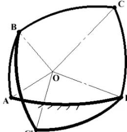
Based on burmester theory for spherical problems, the cir-cle points are calculated by kinematic analysis of 4R linkage constructed by image poles. The theory is explained by Shi-razi (2005), as shown in Fig. 2. When the driving link of 4R linkage constructed by poles (which is denoted by Pij) and
image poles (which is denoted by P1ij) rotates the angleω, the 4R linkage moves from the orientation P12P13P134P124to
P12P13P1 0 34P1
0
24. The circle point C1is determined by the
in-tersection of sphere and two planes PM and PN, the plane PM
is defined by the center point of sphere (which is denoted by point O) and normal vector P124 P1240, the point PN is defined
by the center point of sphere and normal vector P134P1340. For each circle point C1, the center point C0is obtained as
following steps. Firstly, define a point P123 as the reflection
point of C1relative to the plane POP12P13. The plane POP12P13
is defined by the center point of sphere, the pole P12and P13.
And define the point P124 as the reflection point of C1
rela-tive to the plane POP12P14, the plane POP12P14is defined by the
center point of sphere, the pole P12and P14. Relative to the
plane POP12P23, the circle point at the second specified
orien-tation C2is the reflection point of P123. POP12P23is defined by
the center point of sphere, the pole P12 and P23. Relative to
the plane POP13P23, the circle point at the third specified
ori-entation C3is the reflection point of P123. POP13P23 is defined
by the center point of sphere, the pole P13 and P23.
Rela-tive to the plane POP14P24, the circle point at the fourth
speci-fied orientation C4is the reflection point of P124. POP14P24is
defined by the center point of sphere, the pole P14 and P24.
Then, the center point C0is determined by the intersection
of the sphere and any two perpendicular bisector planes of C1C2, C1C3and C1C4. With the rotation of the driving link
of 4R linkage P12 P13 P134 P124, a series of circle points or
Figure 1.The flow chart of the linkage synthesis calculation.
points and circle points are obtained for each new orienta-tion of linkage P12P13P134P124, and they are both valid and
symmetrical for the center point of sphere.
In order to realize the calculation and visualization of link-age synthesis mentioned above, a series of functions on geo-metric calculation are defined in this program package, such as the calculation functions on rotation, mirror, intersection.
4 Calculation and analysis of the linkage solution
4.1 Circuit defect discrimination
Figure 2.Principle of the spherical 4R linkage synthesis (reproduced from Shirazi, 2007).
Figure 3.Spherical 4R linkage located at the limited orientations.
of driving link should be calculated firstly. Figure 3 shows a configuration of spherical triangle which is changed from spherical 4R linkage ABCD(P), where P is the guiding point on the coupler link BC; P1–P4are the given four guiding
ori-entations;α–γandθ1∼θ4represent the length and roll angle
of each link of spherical linkage respectively;δrepresents the angle between the link BC and BP. The point coordinates of sphere are defined by longitude θand latitudeϕ, for exam-ple, the coordinates of the point A can be expressed as (θA,
ϕA).
For the configuration of spherical triangle A(BC)D, define a=η+β,b=γ,c=αandp=(a+b+c)/2, the limited angles of driving link withθ4=0 is calculated by the
half-angle formula
sin 6 A
2 = r
sin (p−b) sin (p−c) sinbsinc cos
6 A 2 =
r
sinpsin (p−a) sinbsinc
(1)
where6 Arepresents the angle from the link AD to the link AB. In addition, the angleθ4can be expressed as
sinθ4=
cosφDsin (θA−θD)
sinγ cosθ4=
sinφD−sinφAcosγ
cosφAsinγ
(2)
Then, the limited angles of driving link which is denoted by θ1+andθ1−can be calculated as
θ1+ =2 arctan 2
sin 6 A
2 ,cos 6 A
2
+arctan 2 (sinθ4,cosθ4)
θ1− = −2 arctan 2
sin 6 A
2 ,cos 6 A
2
+arctan 2 (sinθ4,cosθ4)
(3)
If there is no real root in Eq. (1), the calculation will be in-valid, and the set of the limited angles of the driving link (which is denoted byθ11∗) will be empty, that isθ11∗ = [ ]. If not,θ11∗ = [θ1+, θ1−].
Similarly, for the configuration of spherical triangle A(B0C0)D, definea= |η−β|,b=γ,c=αandp=(a+b+ c)/2. If there is no real root in Eq. (1), the calculation will be invalid, and the set of the limited angles of the driving link (which is denoted byθ12∗) will be empty, that isθ12∗ = [ ]. If not,θ12∗ = [θ1+, θ1−].
The final set of the limited angles of driving link denoted by θ1∗, consider θ1∗=θ11∗ ∪θ12∗. Obviously, the size of θ1∗ which is denoted byN1∗ is only 0, 2 or 4. Due to the driv-ing link can’t move between two adjacent movdriv-ing intervals, the circuit defect can only be checked whenN1∗=4. In this case, if all input angles of the driving link are corresponding to the specified coupler orientations located at the same mov-ing interval, the linkage solution will be valid. If not, there will be a circuit defect in the motion of spherical 4R linkage. Specially, the input angle of driving link is expressed as
sinθ1=
cosφBsin (θA−θB)
sinα cosθ1=
sinφB−sinφAcosα
cosφAsinα
(4)
4.2 Branch defect discrimination
Figure 4.Constructions of the driven link of spherical 4R linkage.
jamming, a branch defect will appear once the driven link in given four coupler orientations locates at different assembly configurations. Actually, the branch of linkage is determined by the solution of motion equation of driven link.
According to the coordinate of point A(θA, ϕA), the length
of AB (that is α) and the roll angle of AB (that is θ1), the
coordinate of point B(θB, ϕB) is expressed as
sinφB=cosαsinφA+sinαcosθ1cosφA
sinθB=
−sinαsinθ1cosθA+cosαsinθAcosφA
−sinαcosθ1sinθAsinφA
cosφB
cosθB=
sinαsinθ1sinθA+cosαcosθAcosφA
−sinαcosθ1cosθAsinφA
cosφB
(5)
Similarly, the coordinate of point C(θC, ϕC) can be expressed
as
sinφC=cosβsinφD+sinβcosθ3cosφD
sinθC=
−sinβsinθ3cosθD+cosβsinθDcosφD
−sinβcosθ3sinθDsinφD
cosφC
cosθC=
sinβsinθ3sinθD+cosβcosθDcosφD
−sinβcosθ3cosθDsinφD
cosφC
(6)
The relationship between point B and C is determined by the length of link BC (that isη), that is
cosη=sinφBsinφC+cosφBcosφCcos (θB−θC) (7)
Substitute the Eqs. (5) and (6) into Eq. (7) and obtain follow-ing equation, that is
τ1sinθ3(θ1)+τ2cosθ3(θ1)+τ3=0 (8)
Where
τ1 =λ1sinβsinθD−λ2sinβcosθD
τ2 = −λ1sinβcosθDsinφD−λ2sinβsinθDsinφD
+λ3sinβcosφD
τ3 =λ1cosβcosθDcosφD+λ2cosβsinθDcosφD
+λ3cosβsinφD−cosη
λ1 =sinαsinθ1sinθA+cosαcosθAcosφA
−sinαcosθ1cosθAsinφA
λ2 = −sinαsinθ1cosθA+cosαsinθAcosφA
−sinαcosθ1sinθAsinφA
λ3 =cosαsinφA+sinαcosθ1cosφA
(9)
According to above equations, the output angleθ3+ obtains two roots that isθ3+andθ3−, which can be calculated as
θ3+(θ1)=2 arctan
τ1+
q
τ12+τ22−τ32 τ2−τ3
θ3−(θ1)=2 arctan
τ1−
q
τ12+τ22−τ32 τ2−τ3
(10)
For each location of driving link corresponded to four spec-ified coupler orientations, if all actual output anglesθ3 are
generated by the same subformula of Eq. (10), the linkage solution will be valid. If not, a branch defect will appear in the motion of spherical 4R linkage. Specially, according to the coordinates of point C and D, the actual output anglesθ3
can be calculated by the method of Eq. (4).
4.3 Order defect discrimination
The order defect occurs when the coupler link can’t pass the given four-orientations with the order of 1–2–3–4 or 4–3– 2–1. Obviously, if the driving link is rotated fully, the geo-metrical criterionθ21< θ31< θ41orθ21> θ31> θ41will be
used to solve this problem according to the definition of or-der defect, whereθj irepresents the rotation angle of driving
link revolves from orientation ABi (which is corresponded to coupler orientationi) to ABj (which is corresponded to coupler orientationj) round the axis OA, as shown in Fig. 5. In order to obtain rotation angleθj i, the normal vector of
plane OABi (which is denoted byn1) and OABj (which is
denoted byn2) are expressed asn1=OA×OBi,n2=OA×
OBj. Based on the conclusions, the normal vector of axis OA in plane OABi (which is denoted byf1) and plane OABj
(which is denoted byf2) are expressed asf1=n1×OA,f2=
n2×OA. Define OA= [x1, y1, z1], andf1×f2= [x2, y2, z2].
The rotation angle of driving linkθj iis calculated as
θj i=arccos
f1·f2
|f1| |f2| z1·z2>0 θj i=2π−θj i others
(11)
On the contrary, if the driving link is rotated partially, the geometrical criterion which mentioned above (that isθ21<
Figure 5.Driving link revolved round the pole axis of sphere.
Figure 6.Order defect discrimination.
the order 4–1–2–3 is incorrect because of the driving link can’t move from one moving interval to other, as shown in Fig. 6. In this case, the geometrical criterion is modified asθ1e< θ2e< θ3e< θ4e orθ1e> θ2e> θ3e> θ4e, where the
subscript lettererepresents the arbitrary limited orientations of the driving link.
4.4 Pyramid structure of the motion defect calculation The method of defect discrimination cannot be considered in isolation. For example, the calculation on the order de-fect discrimination is meaningless for a 4R linkage with cir-cle defect because the coupler of the 4R linkage cannot pass through all specified orientations. In order to solve this prob-lem, a pyramid structure is defined in this program pack-age. The circuit defect locates at the bottom of pyramid, the branch defect locates at the middle of pyramid, and the or-der defect locates at the top of pyramid. Unor-der this defi-nition, both the circuit defect and branch defect should be checked first before the calculation of order defect
discrim-Table 1.Classification of the linkage type (Murray and Larochelle, 1998).
K1 K2 K3 K4
Crank rocker +(−) +(−) +(−) +(−) Rocker crank +(−) −(+) −(+) +(−) Double crank −(+) −(+) +(−) +(−) Grashof double rocker −(+) +(−) −(+) +(−) 00 double rocker −(+) −(+) −(+) +(−) 0πdouble rocker +(−) +(−) −(+) +(−) π0 double rocker +(−) −(+) +(−) +(−) π πdouble rocker −(+) +(−) +(−) +(−)
ination. Similarly, the circuit defect should be checked first before the calculation of branch defect discrimination.
4.5 Linkage type classification
For a number of synthesis tasks, the 4R linkage with spec-ified linkage type should be satisfied. According to the method proposed by Murray, there are 8 kinds of linkage type for a spherical 4R linkage, as shown in Table 1, where K1=γ−α+η−β,K2=γ−α−η+β,K3=η+β−γ−α,
K4=2π−η−β−γ−α. Specially, at least one link of a 4R
linkage will be rotated fully ifK1K2K3K4>0, which is the
Grashof’s condition. Both calculations on the linkage type and Grashof’s condition are supported by program package.
4.6 Performance evaluation and solutions domain analysis
A standard function interface on linkage performance calcu-lation is provided for the designer in the program package. The input vector of this function is a data structure to de-scribe the coordinate information of linkage solution at each specified orientation, and the output variable of this function is a real number to indicate the linkage performance. If there are more than one evaluating indicators for the linkage per-formance, a weight method will be used. Of course, all the functions in the program package can be called in this func-tion.
Actually, a default function template is provided for the designer. The evaluating indicator which defined in this func-tion template is termed as “Braking angle”. For a valid 4R linkage solution which driving link is rotated partially, if the rotation angle of driving link from the specified orientation 1 (or 4) to the nearest limited orientation is too small, the driving link will be difficult to stop before the linkage moves to the limited orientation for the reason of the high rotation speed or the inaccurate displacement control of the motor.
Figure 7.Constructions of solutions map.
distribution of the linkage performance evaluation in the so-lution domain will be obtained. The calculation on the solu-tions domain analysis is visualized by a solusolu-tions map, which is introduced later.
5 Synthesis visualization
5.1 Task visualization
Once the four coupler orientations is specified, a figure with four orientations, the center points and the circle points plot-ted in a sphere are generaplot-ted. The designer can adjust task parameters according to the figure. The specified coupler ori-entations are defined by four equilong arcs in the sphere, and the longitude and latitude of the coupler orientation are determined by the starting point of arc, and the roll an-gle of coupler orientation is determined by the roll anan-gle of arc. Specially, in order to plot the arc in the surface of sphere smoothly, the arc is divided into several line segments through an interpolation method.
5.2 Solutions map
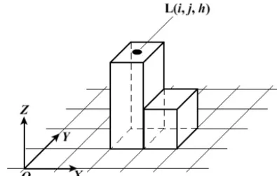
ForN center points and circle points, all linkage solutions can be mapped into a three-dimensional coordinate system O−XY Z, that is the visualization of solutions domain analy-sis mentioned above. In this coordinate system,N×Ncubes are constructed based on theO−XY plane, and each link-age solution defined by the center point (or circle point) i and the center point (or circle point)j is described by a cube L(i, j, h), as shown in Fig. 7, whereiis thexoffset of cube L,j is theyoffset of the cubeL,his thezoffset of the cube L,iandjare determined by selected center points (or circle points), andhis determined by linkage performance. In or-der to describe the linkage type of solution, each cube in the solutions map is color-coded according to linkage type.
5.3 Solutions visualization
The key problem of solutions visualization is the motion analysis and calculation of coupler curve. Figure 3 shows that
the output angleθ3is calculated by the Eq. (10) aimmed at
each input angleθ1. Due to the coordinates of point A and
D of spherical 4R linkage are given, the coordinates of point B and C can be obtained according to the Eqs. (5) and (6). Then, the rotation angle of link BC (that isθ2) can be
calcu-lated as
sinθ2=
cosφCsin (θB−θC)
sinη cosθ2=
sinφC−sinφBcosη
cosφBsinη
(12)
Correspondingly, the rotation angle revolved from the link BC to BP (that isδ) is obtained by the rotation method intro-duced in Sect. 3.3. Obviously, the angleδis a constant value and calculated from the coordinate information of spherical 4R linkage at any specified orientations. On this basis, the rotation angle of link BP (denoted byθ5) is “θ2+δ”, and the
coordinate of point P is expressed as
sinφP=cosκsinφB+sinκcosθ5cosφB
sinθP=
−sinκsinθ5cosθB+cosκsinθBcosφB
−sinκcosθ5sinθBsinφB
cosφP
cosθP=
sinκsinθ5sinθB+cosκcosθBcosφB
−sinκcosθ5cosθBsinφB
cosφP
(13)
According to the calculation above, the point coordinates of the spherical 4R linkage under each input angle are calcu-lated, and the coordinate data is applied to conduct the ani-mation of linkage motion and plot the coupler curve. Due to there are two solutions in the Eq. (10) corresponding to the two assembly configurations of spherical 4R linkage driven link, the coupler curve is generated at twice. In order to dis-tinguish the branch of coupler curve, different colors are used to represent different branches. Specially, for a spherical 4R linkage which driving link rotated partially, each solution of Eq. (10) should be checked because there is no real root for some input angles of driving link.
6 Expansion of the program package on planar 4R linkage
The synthesis on both spherical and planar 4R linkages is supported by the program package. The calculation on spher-ical problem mentioned above is mainly based on the the-ory of spherical trigonometry (Ratcliffe, 2006). Actually, the geometrical principle of planar 4R linkage is similar to a spherical one. As the Fig. 2 shows, the spherical 4R link-age only move along the surface of a sphere and all the axes of hinges passes through the center of sphere. If the diameter of sphere is infinite, the spherical 4R linkage ABCD will be transformed into a planar one.
For the discrimination of linkage circuit defect, the dif-ference between spherical and planar problems is the cal-culation of limited orientations of driving link, which can be obtained by the cosine theorem of planar triangle. Define a0= |BC| + |CD|,b0= |AD|,c0= |AB|, if the configuration of planar triangle is A(BC)D, the limited angles of driving link which is denoted byθ11∗andθ12∗could be calculated as
θ1∗
1 =arccos
c02+b02−a02 2c0b0
!
+arctan 2 (sinθ4,cosθ4)
θ12∗= −arccos c
02
+b02−a02 2c0b0
!
+arctan 2 (sinθ4,cosθ4)
(14)
Similarly, if the configuration of planar triangle is A(B0C0)D, the Eq. (14) will be applicable as a= |BC| − |CD|. If it is not all input angles of driving link corresponding to the spec-ified coupler orientations locates at the same moving inter-val, the linkage solution will be invalid. Specially, the valid-ity of Eq. (14) is determined by the validvalid-ity of expression v=(c2+b2−a2)/2cb. If the solution of Eq. (14) is valid, the conditionv∈ [−1,1]should be satisfied.
For the discrimination of linkage branch defect, the Eqs. (8) and (10) are applicable, the difference between spherical and planar problems is the expression ofτ1,τ2,τ3,
where
τ1 =2|AB| |CD|sinθ1−2|AD| |CD|sinθ4
τ2 =2|AB| |CD|cosθ1−2|AD| |CD|cosθ4
τ3 = |BC|2− |AB|2− |CD|2− |AD|2
+2|AB| |AD|cos (θ1−θ4)
(15)
If it was not all actual output anglesθ3corresponding to four
specified coupler orientations that could be generated by the same subformula of Eq. (14), the linkage solution would be invalid.
For the discrimination of linkage order defect, the geo-metrical criterionθ21< θ31< θ41orθ21> θ31> θ41for
link-age with rotating fully driving link and geometrical crite-rionθ1e< θ2e< θ3e< θ4e orθ1e> θ2e> θ3e> θ4e for
link-age with rotating partially driving link are applicable. The difference between spherical and planar problems is the vec-tors f1 andf2 in the Eq. (11), wheref1=ABi andf2=
ABj.
For the classification of linkage type and the condition of grashof, the method proposed by Martin and Murray (2002) is applicable to planar 4R linkage. For the performance eval-uation, the “Braking angle” of planar 4R linkage is obtained from the calculation on planar vectors. Similarly, for the syn-thesis visualization of planar 4R linkage, the method men-tioned in Sect. 4 is applicable, and the calculation is based on the principle of planar trigonometry.
Figure 8.Center points and circle points generated by the program package.
Figure 9.Solutions map generated by the program package.
7 Examples
7.1 Spherical 4R linkage synthesis
In this example, it is necessary to synthesize a spherical 4R linkage to guide a camera to pass four specified orientations without circuit defect, branch defect and order defect, as shown in Table 2.
Figure 10.Solutions visualization.
Table 2.Specified coupler orientations for a spherical 4R linkage.
Orientation Longitude (◦) Latitude (◦) Roll (◦)
P1 10 0 −4
P2 40 −20 1
P3 75 −10 4
P4 130 15 5
therefore, only the solutions with a type of double crank need to be considered.
The program allows designer to select valid solutions on the solutions map directly, and this way is quick and effi-cient. As the Fig. 9 shows, a candidate solution is selected from region I of solutions map, and the solution information is shown in Table 3. Similarly, another three linkage solutions selected from region II–IV of solutions map are erased be-cause of motion defect, and the solution information is shown in Table 3. In order to verify the results, the plotting program is called to generate coupler curve of four linkages, as shown in Fig. 10. Obviously, only the linkage solution I is feasible.
In this calculation, 7396 groups of linkage solutions are synthesized and analyzed. When the program is running on the computer, it takes 4.48 s to generate and display the so-lutions map at one time. In the process of linkage solution selection, it only takes 0.37 s to generate and display the cou-pler curve of the selected linkage solution each time.
7.2 Planar 4R linkage synthesis
In this example, it is necessary to synthesize a planar 4R linkage to guide the bucket of the skid steer loader to pass four specified orientations without circuit defect, branch de-fect and order dede-fect, as shown in Table 4.
Firstly, the synthesis program is called to generate cen-ter points and circle points, the result is shown in Fig. 11. Then, the solutions map is generated, the result is shown in Fig. 12. It is noted that the installation position of the 4R linkage on the skid steer loader is limited, which becomes a strong constraint condition for the rationality of the solution.
Figure 11.Center points and circle points generated by the program package.
In order to provide enough candidate solutions, this exam-ple no longer calculates the transmission performance of the linkage solution, but loads the picture of the skid steer loader with reduced proportion into the drawing area to evaluate the reasonableness of the installation position of the linkage so-lution.
Table 3.Solutions information.
No. A(θA, ϕA) (◦) B(θB, ϕB) (◦) C(θC, ϕC) (◦) D(θD, ϕD) (◦) Defection type Linkage type
I 2.7341, 65.4782 −39.3638, 67.3055 −49.9400, 68.4720 −4.1762, 67.9088 No defect Double crank II 6.0954, 64.7366 −34.2196, 67.5189 −85.6241, 80.5367 −31.0304, 73.7294 Circle defect Roker crank III 21.0157, 72.8766 35.1467, 83.0991 −63.4609, 73.7618 −13.2424, 71.8844 Branch defect 0πdouble rocker IV 6.0954, 64.7366 −34.2196, 67.5189 −68.0395, 75.9051 −16.5879, 72.9075 Order defect 00 double rocker
Table 4.Specified coupler orientations for a planar 4R linkage.
Orientation Abscissa (mm) Ordinate (mm) Roll (◦)
P1 −112 246 0
P2 −179 1260 −15.8
P3 −239 2060 −26.5
P4 −277 2838 −39.1
Figure 12.Solutions map generated by the program package.
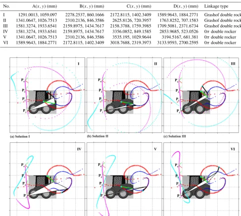
III–VI is outside the body of the skid steer loader. Obviously, only the installation position of the rocker with solution I is reasonable and meets the requirements of linkage synthesis.
In this calculation, 19 600 groups of linkage solutions are synthesized and analyzed. When the program is run on the computer, it takes 12.73 s to generate and display the solu-tions map at one time. In the process of linkage solution se-lection, it only takes 0.24 s to generate and display the cou-pler curve of the selected linkage solution each time.
8 Concluding remarks
In this paper, a synthesis program package is developed to find a satisfied planar or spherical linkage solution
automat-ically according to burmester theory. The main conclusions of this study are as follows:
1. The program package developed in this paper has fast calculation speed and high synthesis efficiency. The time required for synthesis calculation depends on the segmentation accuracy of buermester center curve, that is, the rotation angle increment of driving link of 4R linkage constructed by image poles when generating each center point. The more precise the burmester cen-ter curve is segmented, the more solutions are gener-ated and the longer the calculation time is. In the two examples given in this paper, the number of linkage so-lutions analyzed is 7396 and 19 600 respectively, and the total time required for solutions map generation and display is 4.48 and 12.73 s respectively. The generation of the solutions map is one-time, after which the selec-tion and analysis of linkage soluselec-tion only takes less than 0.5 s each time. In addition, the solutions map proposed in this study extends the dimension of traditionaltype map, so that it can also express the transmission per-formance of linkage solutions while expressing linkage types. This method further avoids the blindness of link-age synthesis.
2. The proposed defect discrimination algorithm is not only correct but also logical. In the synthetic example of spherical 4R linkage, by comparing the result of pro-gram discrimination with that of coupler curve analy-sis, it can be seen that the algorithm in this paper can correctly discriminate the defect of circuit, branch and order. Moreover, this paper proposes a pyramid struc-ture for defect discrimination. This is obviously more logical. For example, when four given orientations are located in different circuits and branches, the coupler curve of 4R linkage can not pass through all four ori-entations at all. It is not logical to discuss whether the coupler link can pass through four orientations orderly.
cal-Table 5.Solutions information.
No. A(x, y) (mm) B(x, y) (mm) C(x, y) (mm) D(x, y) (mm) Linkage type
I 1291.0013, 1059.097 2278.2537, 860.1666 2172.8115, 1402.3409 1589.9643, 1884.2771 Grashof double rocker II 1341.0647, 1026.7513 2310.2136, 846.3586 2625.8126, 720.3957 1763.8252, 707.1583 Grashof double rocker III 1581.3274, 1933.6541 2159.8975, 1434.7617 2158.3788, 1759.3985 1709.5081, 2371.6734 Grashof double rocker IV 1581.3274, 1933.6541 2159.8975, 1434.7617 3356.0852, 849.1585 2853.9685, 523.0526 0πdouble rocker V 1341.0647, 1026.7513 2310.2136, 846.3586 3535.195, 1029.9644 3194.5167, 681.381 0πdouble rocker VI 1589.9643, 1884.2771 2172.8115, 1402.3409 3018.7688, 2319.3973 3133.9593, 2700.2595 0πdouble rocker
Figure 13.Solutions visualization.
culation, but also reorganize these functions to solve more complex problems.
Considering that the precise orientation synthesis problem and the function synthesis problem can be transformed each other, how to extend the research method in this paper, espe-cially the defect discrimination method, to the function syn-thesis field of spherical and planar 4R linkage is the next re-search direction of this paper.
Data availability. All the data used in this paper can be obtained by request from the corresponding author.
Author contributions. GW suggested the overall concept of this paper and completed the development of the program package based on Matlab. HZ, XL and JW worked together to complete the examples used in this paper. XZ and GF edited and verified all the formulas and pictures used in this paper.
Competing interests. The authors declare that they have no con-flict of interest.
Program (Project no. 2018GNC112008), and the Funds of Shan-dong “Double Tops” Program (Project no. SYL2017XTTD14).
Financial support. This research has been supported by the National Key Research and Development Program (grant no. 2016YFD0701103), the Shandong Key Research and Development Program (grant no. 2018GNC112008), and the Shandong “Double Tops” Program (grant no. SYL2017XTTD14).
Review statement. This paper was edited by Doina Pisla and re-viewed by two anonymous referees.
References
Baskar, A. and Bandyopadhyay, S.: A homotopy-based method for the synthesis of defect-free mechanisms satisfying secondary design considerations, Mech. Mach. Theory, 133, 395–416, https://doi.org/10.1016/j.mechmachtheory.2018.12.002, 2019a. Baskar, A. and Bandyopadhyay, S.: An algorithm to compute the
finite roots of large systems of polynomial equations arising in kinematic synthesis, Mech. Mach. Theory, 133, 493–513, https://doi.org/10.1016/j.mechmachtheory.2018.12.004, 2019b. Bai, S.: Geometric analysis of coupler-link mobility and circuits
for planar four-bar linkages, Mech. Mach. Theory, 118, 53–64, https://doi.org/10.1016/j.mechmachtheory.2017.07.019, 2017. Chanekar, P. V., Fenelon, M. A. A., and Ghosal, A.:
Synthe-sis of adjustable spherical four-link mechanisms for approxi-mate multi-path generation, Mech. Mach. Theory, 70, 538–552, https://doi.org/10.1016/j.mechmachtheory.2013.08.009, 2013. Erdman, A. G. and Loftness P. E.: Synthesis of linkages for
cataract surgery: storage, folding, and delivery of replacement intraocular lenses(IOLs), Mech. Mach. Theory, 40, 337–351, https://doi.org/10.1016/j.mechmachtheory.2004.07.006, 2005. Filemon, E.: Useful ranges of centerpoint curves for design of
crank-and-rocker linkages, Mech. Mach. Theory, 7, 47–53, https://doi.org/10.1016/0094-114X(72)90015-8, 1972.
Gupta, K. C. and Beloiu, A. S.: Branch and circuit defect elim-ination in spherical four-bar linkages, Mech. Mach. Theory, 33, 491–504, https://doi.org/10.1016/S0094-114X(97)00078-5, 1998.
Han, J. and Cao, Y.: Analytical synthesis method-ology of RCCC linkages for the specified four poses, Mech. Mach. Theory, 133, 531–544, https://doi.org/10.1016/j.mechmachtheory.2018.12.005, 2019. Han, J., Yang, T., Yin, L., and Qian, W.: Modern synthesis theory
and method of linkage mechanism – analytical theory, domain solution method and software system, Higher Education Press, Beijing, China, 2013.
Martin, D. T. and Murray, A. P.: Developing classifications for syn-thesizing, refining, and animating planar mechanisms, ASME 2002 Design Engineering Technical Conferences and Comput-ers and Information in Engineering Conference, 29 September–2 October 2002, Montreal, 2002.
McCarthy, J. M.: 21st Century Kinematics, Springer, London, 2013.
Murray, A. P. and Larochelle, P. M.: A classification scheme for planar 4R, spherical 4R, and spatial RCCC linkages to facilitate computer animation, 1998 ASME Design Engineering Technical Conferences, 13–16 September 1998, Atlanta, 1998.
Myszka, D. H., Murray, A. P., and Schmiedeler, J. P.: Assessing position order in rigid body guidance: an intuitive approach to fixed pivot selection, J. Mech. Design, 131, 0145021–0145025. https://doi.org/10.1115/1.3013851, 2009.
Ratcliffe, J. G.: Foundations of Hyperbolic Manifolds, Springer, New York, 2006.
Mendoza-Trejo, O., Cruz-Villar, C. A., Peón-Escalante, R., Zambrano-Arjona, M. A., and Peñuñuri, F.: Synthesis method for the spherical 4R mechanism with minimum center of mass acceleration, Mech. Mach. Theory, 93, 53–64, https://doi.org/10.1016/j.mechmachtheory.2015.04.015, 2015. Ruth, D. A. and McCarthy, J. M.: The design of spherical 4R
linkages for four specified orientations, Mech. Mach. Theory, 34, 677–692, https://doi.org/10.1016/S0094-114X(98)00048-2, 1999.
Shirazi, K. H.: Synthesis of linkages with four points of accu-racy using Maple-V, Appl. Math. Comput., 164, 731—755, https://doi.org/10.1016/j.amc.2004.04.085, 2005.
Shirazi, K. H.: Computer modelling and geometric construction for four-point synthesis of 4R spheri-cal linkages, Appl. Math. Model., 31, 1874–1888, https://doi.org/10.1016/j.apm.2006.06.013, 2007.
Su, H. J. and McCarthy, J. M.: The synthesis of an RPS serial chain to reach a given set of task positions, Mech. Mach. Theory, 40, 757–775, https://doi.org/10.1016/j.mechmachtheory.2005.01.007, 2005. Sun, J., Chen, L., and Chu, J.: Motion generation of
spherical four-bar mechanism using harmonic charac-teristic parameters, Mech. Mach. Theory, 95, 76–92, https://doi.org/10.1016/j.mechmachtheory.2015.08.020, 2016. Tipparthi, H. and Larochelle, P.: Orientation order analysis of
spherical four-bar mechanisms, J. Mech. Robot., 3, 0445011– 0445014, https://doi.org/10.1115/1.4004898, 2011.
Waldron, K. J. and Strong, R. T.: Improved solutions of the branch and order problems of burmester linkage synthesis, Mecha. Mach. Theory, 13, 199–207, https://doi.org/10.1016/0094-114X(78)90043-5, 1978.
Wang, J., Ting, K. L., and Xue, C.: Discriminant method for the mobility identification of single degree-of-freedom double-loop linkages, Mech. Mach. Theory, 45, 740–755, https://doi.org/10.1016/j.mechmachtheory.2009.12.004, 2010. Zhao, P., Zhu, X., Li, L., Zi, B., and Ge, Q. J.: A