Volume: 01, Issue: 05, Pages: 331-336 (2010)
Performance Modeling in Client Server Network
Comparison of Hub, Switch and Bluetooth
Technology Using Markov Algorithm and
Queuing Petri Nets with the Security Of
Steganography
V.B.Kirubanand, Department of MCA, Sri Krishna College of Engineering and Technology, Coimbatore Dr.S.Palaniammal, Department of Science and Humanities, VLB Janakiammal College of Eng and Tech,
Coimbatore
---ABSTRACT---The main theme of this paper is to find the performance of the Hub, Switch and Bluetooth technology using the Queueing Petri-net model and the markov algorithm with the security of Steganography. This paper mainly focuses on comparis on of Hub, switch and Bluetooth technologies in terms of service rate and arrival rate by using Markov algorithm (M/M(1,b)/1). When comparing the service rates from the Hub network, switch network and the Bluetooth technology, it has been found that the service rate from the Bluetooth technology is very efficient for implementation. The values obtained from the Bluetooth technology can used for calculating the performance of other wireless technologies . QPNs facilitate the integration of both hardware and software aspects of the system behavior in the improved model. The purpose of Steganography is to send the hidden the information from one system to another through the Bluetooth technology with security measures. Queueing Petri Nets are very powerful as a performance analysis and prediction tool. By demonstrating the power of QPNs as a modeling paradigm in further fore coming technologies we hope to motivate further research in this area.
Keywords: Bluetooth, Hub, Switch, Queueing petri-nets, Markov algorithm, Steganography
---Date of Submission: August 08, 2009 Revised: January 29, 2010 Accepted: February 22, 2010
---1. INTRODUCTION
H
ub is a device where the entire connecting mediums come together. A hub is a medium used to collect signals from the input line(s) and redistribute them in various available wirings around a topology (topologies such as: Arcnet, 10base-T, 10base-F etc). Hub basically acts as signal splitter, it accepts signal through its input port and outputs it to the output ports. Some hubs help in regenerating the weak signals prior to sending them to the intended output lines, whereas some hubs help in synchronizing the data communication (in simple words, the hub not only provide the mean of interface within the network, it also provides some additional and useful features). Sometimes multiple hubs are interconnected in the network. Generally hubs are used more commonly where star topology is used [1].Switch is a network switch is a small hardware device that joins multiple computers together within one local area network (LAN). Technically, network switches operate at layer two (Data Link Layer) of the OSI model.[2]
Volume: 01, Issue: 05, Pages: 331-336 (2010)
globally unlicensed Industrial, Scientific and Medical (ISM ) 2.4 GHz short-range radio frequency bandwidth. The Bluetooth specifications are developed and licensed by the Bluetooth Special Interest Group (SIG). The Bluetooth SIG consists of companies in the areas of telecommunication, computing, networking, and consumer electronics [3].
The main objective of these models is to find the following with the usage of Markov algorithm and queueing petrinets with the security of Steganography.
• To find the waiting time. • To find the busy period.
2. QUEUEING NETWORKS
A network consists of a set of interconnected queues. Each queue represents a service station, which serves requests (also called jobs) sent by customers. A service station consists of one or more servers and a waiting area which holds requests waiting to be served. When a request arrives at a service station, its service begins immediately if a free server is available. Otherwise, the request is forced to wait in the waiting area. Service is done as per the general bulk service rule introduced by Neuts (1967) with a=1. As per this rule immediately after the completion of the service, if the server finds a unit present, it start its service; if it finds one or more but almost bit takes them all in a batch and if it finds more than bit takes in the batch for service b units , while others wait. The batch takes a minimum of one unit and a maximum of b units.[4]The time between successive request arrivals is called interarrival time. Each request demands a certain amount of service,
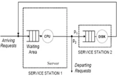
Figure 1: A Basic Queueing Network
which is specified by the length of time a server is occupied serving it, i.e the service time. The delay is the amount of time the request waits in the waiting area before its service begins. The response time is the total amount of time the request spends at the service station, i.e. the sum of the delay and the service time.
Figure 1 shows a basic network with two queues, i.e. service stations. Arriving requests first visit service station 1, which has one servers (representing CPU). After requests are serv ed by the server, they move to service station 2 (representing a disk device) with probability p1 or leave the network with probability p2. Requests completing service at station 2 return back to station 1. The interconnection of queues in a network is des cribed by the paths requests may take which are specified by routing probabilities. A request might visit a service station multiple times while it circulates through the network. The total amount of service time required, over all visits to the station, is called service demand of the request at the station. Requests are usually grouped into classes with all requests in the same class having the same service demands. The algorithm which determines the order in which requests are served at a service station is called scheduling strategy (or scheduling/ discipline).[4] Some typical scheduling strategies are:
-FCFS (First-Come -First-Served): Requests are served in the order in which they arrive. This strategy is typically used for queues representing I/O devices.
-LCFS (Last-Come -First-Served): The request that arrived last is served next.
- PS (Processor-Sharing) All requests are assumed to be served simultaneously with the server speed being equally divided among them. This strategy is typically used for modeling CPUs.
- IS (Infinite-Server): There is an ample number of servers so that no queue ever forms. Service stations with IS scheduling strategy are often called delay resources or delay servers.
3. PETRI NETS
A Petri net is a mathematical representation of discrete parallel systems. Petri nets were defined in the 1960s by Carl Adam Petri. Because of their ability to express concurrent events , they generalize automata theory. A Petri net consists of places, transitions and directed arcs. Arcs connect a place to a transition and vice versa. There are no arcs between two places, nor between two transitions. Places may contain any number of tokens. Transitions fire, that is consume tokens from input positions and produce tokens in output positions. A transition is enabled if there are tokens in every input position. [5]
Volume: 01, Issue: 05, Pages: 331-336 (2010)
A formal definition of queueing petri nets is given below: Definition (PN) An ordinary Petri Net (PN) is a 5-tuple, PN = (P, T, , , ),
Where:
1. P is a finite and non-empty set of places, 2. T is a finite and non-empty set of transitions, 3. P n T = ,
4. , : P x T are called backward and forward incidence functions, respectively,
5. : P à N0 is called initial marking.
The incidence functions and specify the interconnection between places and transitions. If (p,t) > 0, an arc leads from place p to transition t and place p is called an input place of the transition. If (p,t) > 0, an arc leads from transition t to place p and place p is called an output place of the transition. The incidence functions assign natural numbers to arcs, which we call weights of the arcs. When each input place of transition t contains at least as many tokens as the weight of the arc connecting it to t, the transition is said to be enabled. An enabled transition may fire, in which case it destroys tokens from its input places and creates tokens in its output places. The amounts of tokens destroyed and created are specified by the arc weights. The initial arrangement of tokens in the net (called marking) is given by the function which specifies how many tokens are contained in each place. When a transition fires, the marking may change. Figure 2 illustrates this using a basic petri net with 4 places and 2 transitions. The Petri net is shown before and after firing of transition , which destroys one token from place p1 and creates one token in place p2.[6]
Figure 2: An Ordinary Petri Net before and after firing transition t1
4. BASIC QUEUEING PETRI NETS
The main idea in the creation of the QPN formalism was to add and timing aspects to the places of Colored Generalized Stochastic Petri Nets.[7] This is done by allowing queues (service stations) to be integrated into places of CGSPNs. A place of a CGSPN which has an
integrated queue is called a place and consists of two components, the queue and a depository for tokens which have completed their service at the queue. This is depicted in Figure 3.
The behavior of the net is as follows: tokens, when fired into a place by any of its input transitions, are inserted into the queue according to the queue's scheduling strategy. Tokens in the queue are not available for output transitions of the place. After completion of its service, a token is immediately moved to the depository, where it becomes available for output transitions of the place. This type of place is called a timed place. Tokens in immediate places can be viewed as being served immediately. Scheduling in such places has priority over scheduling/service in timed places and firing of timed transitions.
Figure 3: A Queueing Place and its Shorthand Notation An enabled timed transition fires after an exponentially distributed delay according to a race policy. Enabled immediate transitions fire according to relative firing frequencies and their firing has priority over that of timed transitions. We now give a formal definition of a QPN and then present an example of a QPN model.
Definition (QPN): A Queueing Petri Net (QPN) is a 8-tuple QPN = (P,T,C, , ;M0,Q,W), where:
1. CPN = (P,T,C, , ;M0) is the underlying Colored Petri Net.
2. Q = ( ,…, ) is an array whose entry ,
Denotes the description of a queue taking all colors of C(P) into consideration, if pi is a timed place or
Equals the keyword untimed, if pi is an untimed place. 3. W = ( ,…. ) is an array of functions whose entry
Volume: 01, Issue: 05, Pages: 331-336 (2010) 5. HIERARCHICAL QUEUEING PETRI NETS As already mentioned the main hurdle to the quantitative analysis of QPNs is the fact that most analysis techniques available are based on Markov Chains and are therefore susceptible to the state space explosion problem. More specifically, as one increases the number of queues and tokens in a QPN, the size of the state space of the underlying Markov Chain grows exponentially and quickly exceeds the capacity of today's computers. This imposes a limit on the size and complexity of the models that are analyzable. An attempt to alleviate this problem was the introduction of Hierarchically-Combined Queueing Petri Nets (HQPNs)[8]. The main idea is to allow hierarchical model specification and then exploit the hierarchical structure for efficient numerical analysis. This type of analysis is termed structured analysis and it allows models to be solved, which are about an order of magnitude larger than those analyzable with conventional techniques.
HQPNs are a natural generalization of the original QPN formalism. In HQPNs a place may contain a whole QPN instead of a single queue. Such a place is called a subnet place and is depicted in Figure 4. A subnet place might contain an ordinary QPN or again a HQPN allowing multiple levels of nesting. For simplicity, in this paper we restrict ourselves to two-level hierarchies. We use the term High-Level QPN (HLQPN) to refer to the upper level of the HQPN and the term Low-Level QPN (LLQPN) to refer to a subnet of the HLQPN.
Figure 4: A subnet place and its shorthand notation Every subnet of a HQPN has a dedicated input and output place, which are ordinary places of a colored Petri Net. Tokens being inserted into a subnet place after a transition rings are added to the input place of the corresponding HQPN subnet. The semantics of the output place of a subnet place is similar to the semantics of the depository of a place: tokens in the output place are available for the output transitions of the subnet place. Tokens contained in all other places of the HQPN subnet are not available for the output transitions of the subnet place [9]. Every HQPN subnet also contains actual ¡
population place, which is used to keep track of the total number of tokens fired into the subnet place.
6. MARKOV ALGORITHM
A Markov algorithm is a variant of a rewriting system, invented by mathematician Andrey Andreevich Markov Jr. in 1960. Like a rewriting system, a Markov algorithm consists of an alphabet and a set of productions. Furthermore, rewriting is done by applying productions one at a time, if any. However, unlike a rewriting system, applications of productions are regulated, in the following sense:
Ø P is ordered so that, among all applicable productions in a single rewriting step, the first applicable one x y must be used;
Ø among all occurrences where rewriting can take place with respect to x y , the leftmost occurrence must be applied.
Formally, a Markov algorithm is a quadruple,
µ=(?,P,F,T)
where
• is an alphabet;
• P is a non-empty finite ordered set (ordered by, say, ) of pairs of words over , whose elements are called productions, and are usually written x y rather than (x y) ;
• F is a subset of P , whose elements are called the final productions; and
• T is a subset of , called the terminal alphabet.[10]
BULK SERVICE RULES (Markov Algorithm)
There could be a number of a policies or rules according to which batches for bulk service may be formed. The following are the types of bulk service policies or rules frequently discussed in the literature.
Volume: 01, Issue: 05, Pages: 331-336 (2010)
The rule with a fixed batch size k has been considered by Fabens, Takacs and others . In this case the server waits until there are k units, and serves all the k units in a batch. If there are more than k waiting when the server becomes free, he takes a batch k for service , while others wait.
Neuts considers the general bulk service rule: if, immediately after the completion of a service, the server finds less than a units present, he waits until there are a units, whereupon he takes the batch of a units for service; if he finds a or more but atmost b,he takes them all in a batch and if he finds more than b,he takes in the batch for service b units , while others wait. The batch takes a minimum of a units and a maximum of b units
Bhat considers the rule that the number taken in a batch is a random variable y. The corresponding Markov model is denoted by M/M^(y)/1.
There are actual situations where one rule seems to be better suited or to be more appropriate than the others.
Performance measures
(i) Probability that the server is idle
= = ,
(ii) Probability that the server is busy and n units in the system
, n=0,1,2,..
(iii)Waiting Time Density v(t)=
(iv)Expected Waiting Time Density E(T)=
(v)Expected Busy Period =
From the above formulas the Performance of Client-Server model can be calculated.
A comparative study of the wired technology with the wireless technology has been done with help of the markovian model M/M(1,b)/1
PARTICULARS HUB
(in sec )
SWITCH (in sec)
BLUETOOTH (in sec)
-Arrival Rate 1/3 1/3 1/3
µ-Service Rate 1/2.4 1/2.32 1/1.8
E(T)-Expected waiting time
0.9123 0.8818 0.6841
E(B)-Expected busy period
3.428 3.3200 2.571
The probability that the server is idle and the probability that the server is busy are same for both of the networks.
? -
Arrival rate, E(T) - Expected waiting time, µ - Service rate, E(B) - Expected busy period. Conclusion
Thus this research work concludes that the performance of the client server architecture is better in the Bluetooth technology when compared to Hub network and we hope to motivate further research in this area.
References
[1]. www.buzzle.com
[2]. www.compnetworking.about.com [3]. www.bluetooth.com
[4]. performance modeling of distributed e-business application using queueing petri nets.By-Kounev,S.;Buchmann,A.,2003
[5]. www.knowledgerush.com
[6]. G. Bolch, S. Greiner, H. De Meer, and K. S. Trivedi. Queueing Networks and Markov Chains -Modelling and Performance Evaluation with Computer Science Applications. Wiley, NewYork, 1998.
Volume: 01, Issue: 05, Pages: 331-336 (2010)
[8]. F. Bause, P. Buchholz, and P. Kemper. Hierarchically Combined Queueing Petri Nets. In Proc. of 11th Intl. Conference on Analysis and Optimization of Systems, Discrete event Systems , Sophie-Antipolis (France), 1994.
[9]. Petri Net, Theory and Applications Edited by Vedran Kordic
[10]. www.planetmath.org
[11].
Stochastic processes. Second edition. J.Medhi. New Age International Publishers.
Authors Biography
V.B.Kirubanand received the M.C.A. degree from Erode Arts & Science College, Erode in 1996.He also obtained his M.phil at Periyar university in 2008 and at present he is pursuing his Ph.D in Anna University, Coimbatore. He worked as lecturer, senior lecturer, instructor and as Head Of the Department in various colleges from 1996 to 2007 and presently he is working as the Head Of the Department of Master of Computer Applications & Software Systems . He has published 21 books regarding computer application and softwares. His area of interest includes network security and wireless networks.