IMAGE FILTERING
Rafia Sultana.A.R
ABSTRACT
The variation of brightness or color information in image results in producing the electronic noise in the image. The precise goal of this paper is to analyse the various methods of filtering out these noises from image using filters. This work was done using MATLAB. At first, a known noise was added to an image and then filtered out using the corresponding method. Later, a random noise was added and then a filtering method was used to remove the noise.
Index Terms: Filtering, Noise, Restoration, Matlab
I.
INTRODUCTION
Images are usually defined as 2-Dimensional functions that carry data and help perceive some particular object [1].
Images can be compared to signals. Hence most of the techniques used on various signals can be applied to
im-ages. In a computer, an image is usually stored as arrays of pixels. Pixels can be called as the smallest constituents
of an Image. Since data is stored in a computer using the bits 1 and 0, Pixel values are usually stores as binary data
varying from 2 bits to 30 bits. An image with a higher resolution usually implies that there is greater number of
bits used to store the value color of that pixel. The number of bits in each pixel used to store data, and to determine
the color depth of the Image. This work will entail research into the effect of noise in an image and the amount of
data that is lost when noise is added. The basic concept is to understand the best possible filter for each type of
noisy image and then find a common algorithm that can filter out more than one type of noise. It is very hard to
create a universal filter that can remove any type of noise. This is because noise is completely random and hence
there is no particular algorithm that can predict noise. Due to the lack of a mathematical formula, or a systematic
approach, one cannot make a single filter that completely removes noise. However, it is possible to combine 2-3
filters and try to remove noise as much as possible. Thus by using a series of filters, a decent amount of image
res-toration can be achieved. Image processing covers a wide range of problems, from edge/line detection to pattern
recognition reconstruction to filtering [2]
II.
STUDY
ON
THE
NOISE
AND
ITS
EFFECTS
At first a statistical analysis was conducted to find out the effect of adding noise, on the spatial domain. This
was done by adding Gaussian noise with different parameters on the same image. Then it was followed by
de-signing an algorithm and implementing it as a program in matlab, such that a decent amount of image
tion would be achieved for any type of noisy image since the main aim was to achieve maximum image
restora-tion.
Procedure
A Simple Lena Image Was taken
Gaussian Noise was added to the image, using parameters
0.4,0.4
3 Gaussian Filters Were Created (3X3, 5X5, 2X2)
All the 3 filters were applied to each of the Noisy Images
Pixel Values of each of the noisy images and the filtered images was compared to the original image in 2
steps
Pixel value 1 == Pixel Value 2
(Pixel value 1) -5 <= Pixel Value 2 <= (Pixel Value 1) +5
Table.1 Noise Range
As Noise is random, all filters may not work on all noisy images. There might be some effect; however, the
amount of image restoration may not be satisficatory.
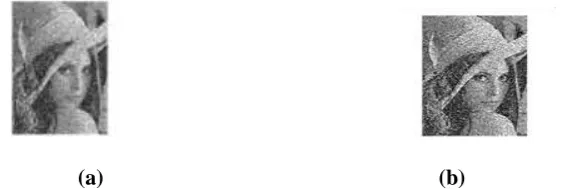
(a) (b)
Figure 1. A) Image with Salt & Pepper Noise and B) Gaussian Blurring on Salt & Pepper on
the Right
III.
KALMAN
FILTERS
IN
IMAGE
PROCESSING
In the early 1960s after a visit to NASA‟s facility, Rudolf E. Kalman, introduced his concept of a very unique filter which
could predict the next state and progressively reach the true values as the amount of input states and information
in-creased. Moreover, it is proved that Kalman process is recursive [3]. One very fundamental way to explain the working
of a Kalman filter would be using an example of a Robot which has a GPS system embedded in it. Assume we have a
Robot “RB” in a huge room. The objective of the Robot would be to pick up random cans of Cola lying around in the
room. The current position of the Robot, could be marked as X. Thus X1, can be the next predicted state. For the next
state, the motor command of the RB would make it go to spot Xa. However, the GPS of RB would indicate that RB is
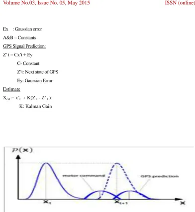
actually at spot Xb. Kalman filters help find the optimum value somewhere in between Xa and Xb. This is demonstrated
in the graph in Figure 2.
Kalman filters essentially have 3 main equations:
State Prediction:
x‟t = Axt-1 + B ut + Ex x‟t : is the next state prediction
Ex : Gaussian error
A&B – Constants
GPS Signal Prediction:
Z‟ t = Cx‟t + Ey
C- Constant
Z‟t: Next state of GPS
Ey: Gaussian Error
Estimate
Xest = x‟t + K(Z t - Z‟ t )
K: Kalman Gain
Figure 2. Graph to predict the Kalman Prediction at t+1
Using a similar principle, Kalman filters can be used to progressively remove noise from any image. If there
exists a base image, the Kalman filter would estimate the next image based on a functioned defined in the
pro-gram, after removing the Gaussian noise present in the image. This, along with the new image, would give a
new estimate to base the next step. Thus by going from one state to the other, the Kalman filter would
eventual-ly yield an image which would be close enough to the original image. Thus, this technology is wideeventual-ly used for
satellite imaging, since satellites take various images over time, and this filter removes noise to a great extent,
thereby giving us very accurate maps.
However, the problem at hand, is that, what if there are just 1 or 2 noisy images to work with?
This yields a major issue, as the amount of image restoration achieved is quite negligible as shown in the
fol-lowing images. This was the main motivation to write a new program in MATLAB, such that a variety of filters
(a)
(b)
Figure 3. (A) Image Shows The Noise Image At State 1, (B) Image On The Right Shows The
Noisy Image At The Next State.
IV.
DESIGN
AND
ALGORITHM
Image processing algorithms consist of a complex sequence of primitive operations, which have to be
per-formed on each nodal value [4]
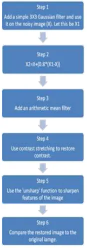
4.1 Overall Process Flow
Using the formula of the second step, it was observed that in the salt and pepper noise, all pepper noise was
removed. It is interesting to note here that, only gain factors between 0.8 and 0.9 worked effectively. Any value
greater or any value lesser than this yielded in residual pepper noise. Since step 3 yielded a great removal of the
pepper noise, leaving behind mostly salt noise, the next natural step, was to create a arithmetic mean
fil-ter(simply averaging filter) [7].
Figure.4 Process Flow For The Algorithm
By applying this filter, almost all of the salt noise was removed. It is also shown that the arithmetic filter works
1) Low contrast
2) Blurring, and hence loss of detail.
At first, to increase the contrast, a simple contrast stretching inbuilt function was used to attain maximum
contrast stretching as possible. To decrease the blurring, the „unsharp‟ inbuilt filter of Matlab was used. The
final image yielded great deal of restoration, as most of the details were obtained back, without much loss, and
on an aesthetic sense, the image restoration was pretty decent.
Description Result
I) Original Image
II) Noisy Image used as
III)Image after applying
Gaussian filter
IV) After Using the
for-mula
X2=X+(0.8*(X1-X))
V) After Using the
arithmetic mean filter
VI)After using contrast
stretching
VII) Restored image after the final step of sharpen-ing the image
4.2
Analysis
It can be well established from the final image that a great degree of image restoration has been achieved.
using the PSNR or Peak Signal to Noise Ratio test. The formula for PSNR is:
MSE =
PSNR = 20 * log10 (255 / sqrt(MSE))
Where, I refers to Original Image, I‟ refers to Noisy Image, MSE refers to Mean Square Error and PSNR refers
to Peak Signal To noise ratio M refers to Number of pixels in each row of the image and N refers to Number of
pixels in each column of the image
When a PSNR test was done on the final restored image, the PSNR value obtained was 24.623dB for the image
both with sharpening and without sharpening. Since a minimum value of 20dB is required for decent image
restoration, the PSNR test conclusively proved the fact that this algorithm was successful. However, since
PSNR compares each pixel value, it is natural to obtain a low PSNR value as masks were used in the program.
Since this greatly changes the values of the pixel, although on an aesthetic level, the image may seem restored,
but there might be quite some difference between the values of the pixels, which is not evident to the human
eye. It was also important to notice whether the program worked well for other types of noises. It was noted that
the image restoration was quite decent and passed the PSNR test for image restoration for both Gaussian noises
and speckle noises
4.3 Shortcomings
The shortcoming of this algorithm is that since a PSNR of atleast 40-50 dB is required for medical images, this
cannot be used as a successful tool for image restoration for medical images. Another problem faced in this
algorithm is that, after applying the unsharp filter, the image does regain quite a few features, yet it becomes
quite grainy. However if the unsharp filter is not used, it looks better aesthetically, yet, has a blurred effect.
V.
CONCLUSIONS
Image restoration has always been a challenge. As mentioned earlier, since noise is random, making one filter
that can completely remove it, is next to impossible. Hence it is important that we use the filters available to
use, in a fashion such that noise is effectively tackled and it can systematically be removed.
The work done on this project has huge scope for improvement, as better PSNR can definitely be achieved with
better use of filters and detailed analysis of the effect of each step on image restoration.
If noise can be removed to an extent that the restored image does not show any signs of additive noise, it can
definitely be used for medical images. This is a challenge, yet can be achieved with detailed research.
REFERENCES
[1] Minh N. Doy, Pier Luigi Dragottiy, Rahul Shuklay, and Martin Vetterliyx, “Paper Title: On the compression of
Two-Dimensional piecewise smooth functions”. In proceeings of IEEE International Conference on Image
Processing (ICIP), 2001.
[2] Hans Knutsson, Filtering and Reconstruction in Image processing, Linköpings Studies in Science and Technology,
[3] Roger M. du Plessis, “Poor Man‟s explanation of Kalman Filtering Or How I stopped worrying and learned love
matrix inversion” North American Rockwell Electronics Group, USA, June 1967
[4] Steffen Klupsch, Markus Ernst, Sorin A. Huss, Martin Rumpf, and Robert Strzodka, “Real time image processing
based on reconfigurable hardware acceleration”. In Proceedings of IEEE Workshop Heterogeneous reconfigurable
Systems on Chip, 2002.
[5] D.Marr, Vision, Freeman, New York, 1982
[6] Fred Weinhaus, Digital Image Filtering, Springer; 2004 edition