R E S E A R C H
Open Access
Confounding and missing data in
cost-effectiveness analysis: comparing
different methods
Tommi H¨ark¨anen
1*, Timo Maljanen
2, Olavi Lindfors
1, Esa Virtala
1and Paul Knekt
1,2Abstract
Introduction: Common approaches in cost-effectiveness analyses do not adjust for confounders. In nonrandomized studies this can result in biased results. Parametric models such as regression models are commonly applied to adjust for confounding, but there are several issues which need to be accounted for. The distribution of costs is often skewed and there can be a considerable proportion of observations of zero costs, which cannot be well handled using simple linear models. Associations between costs and effectiveness cannot usually be explained using observed background information alone, which also requires special attention in parametric modeling. Furthermore, in
longitudinal panel data, missing observations are a growing problem also with nonparametric methods when cumulative outcome measures are used.
Methods: We compare two methods, which can handle the aforementioned issues, in addition to the standard unadjusted bootstrap techniques for assessing cost-effectiveness in the Helsinki Psychotherapy Study based on five repeated measurements of the Global Severity Index (SCL-90-GSI) and direct costs during one year of follow-up in two groups defined by the Defence Style Questionnaire (DSQ) at baseline. The first method models cumulative costs and effectiveness using generalized linear models, multiple imputation and bootstrap techniques. The second method deals with repeated measurement data directly using a hierarchical two-part logistic and gamma regression model for costs, a hierarchical linear model for effectiveness, and Bayesian inference.
Results: The adjustment for confounders mitigated the differences of the DSQ groups. Our method, based on Bayesian inference, revealed the unexplained association of costs and effectiveness. Furthermore, the method also demonstrated strong heteroscedasticity in positive costs.
Conclusions: Confounders should be accounted for in cost-effectiveness analyses, if the comparison groups are not randomized.
JEL classification: C1; C3; I1
Keywords: Clinical trial, Cost-effectiveness analysis, Confounders, Predictive margins, Two-part model, Bayesian inference
*Correspondence: tommi.harkanen@thl.fi
1National Institute of Health and Welfare, Mannerheimintie 166, P.O.Box 30, FIN-00271 Helsinki, Finland
Full list of author information is available at the end of the article
Background
Cost-effectiveness analyses are often based on compar-ing average costs with the effectiveness of the treatments, and on bootstrap methods [1]. Bootstrap methods have been shown to have good properties when compared with parametric methods[2-4]. A standard application of this approach does not adjust for possible confounding effects, which can have a considerable influence on the results not only in observational but also in randomised studies [5]. In randomized controlled trials spurious differences in the distributions of background factors can emerge due to random variation especially with small sample sizes. This can induce a need to adjust for confounding. Some statis-tical methods have been developed to estimate adjusted means using (generalized) linear models, but it seems that these methods have seldom been applied in cost-effectiveness analyses. In the predictive margins approach [6,7] the mean of individual predictions based on a gener-alized linear regression model are calculated, which allows for comparison of different scenarios by modification of the covariate values. In Bayesian inference, predictive dis-tributions (e.g. [8]) can be applied for calculating adjusted means.
Longitudinal data have often been compressed by using different cumulative measures of costs and effectiveness outcomes (e.g. area under curve, AUC). The application of cumulative costs can also reduce the number of obser-vations with zero costs in repeated measurement data and skewness, therefore, reducing the problems related to the application of linear models.
A drawback of cumulative measures is that a missing value in the outcome variable at a given measurement point will result in missing values in the cumulative out-come values of the subsequent measurement points. Mul-tiple imputation (MI) [9] and data augmentation [10] can be applied to deal with missing outcome values at sin-gle measurement points, so that all of the information for the observed outcome values can be utilised for the cumulative outcomes.
The distribution of costs is generally skewed, with a pro-portion of observations having zero costs and the remain-ing portion havremain-ing positive costs. Direct application of linear regression models is not suitable for these kinds of data, because if the model is used to predict costs, the pre-dictions could suggest negative costs or other unrealistic results in some scenarios. The usual method of reducing skewness using logarithmic transformation is not sensible when some of the study subjects have zero costs. Two-part models [11], for example, have been proposed for solving this problem.
Missing values may be present not only in the depen-dent variable but also in the independepen-dent variables in the regression model. These variables can be, for exam-ple, skewed or categorical. Multiple imputation of missing
costs with possibly zero values is more complicated, and two-part models can be more useful. In these cases, meth-ods which assume a multinormal distribution for the variables are not ideal. More suitable methods, which can handle the aforementioned complications, can be based on data augmentation and Bayesian inference and imple-mented, for example, by using the OpenBUGS software [12,13].
In the case of an observational study and non-intervention-based comparison groups based on, for example, a patient characteristic the cost-effectiveness analysis demonstrates the change of the average costs (relative to the change in the average effectiveness). This information allows a decision-maker to plan more cost-effective interventions, as not only different patient-specific characteristics but also other baseline factors can be compared in terms of the standardized average cost differences.
The Helsinki Psychotherapy Study (HPS) is a ran-domised clinical trial comparing three therapy treatments [14]. In addition to comparisons of the randomized ther-apy groups, the data set can be utilized to conduct cost-effectiveness analyses by comparing groups defined by nonrandomized baseline factors, in which case the ran-domization no longer plays any part and confounding fac-tors generally need to be adjusted for. In the present work, we compared two groups based on the Defence Style Questionnaire (DSQ) [15], resulting in the identification of several potential confounders.
The aims of the study were as follows: a) We han-dle confounding by applying predictive margins in the frequentist inference and predictive distributions in the Bayesian inference to produce adjusted means of cost and effectiveness, and their differences. b) We address missing data at single measurements of a repeated mea-surement study by using the multiple imputation and data augmentation techniques. c) We assess the unexplained associations between costs and effectiveness by applying Bayesian hierarchical models. d) We handle nonnega-tive costs by applying a two-part model using a logistic regression model as an indicator of zero or positive costs, and a hierarchical gamma regression model for positive costs to avoid unrealistic negative predictive costs, which can be a result of an application of simple linear mod-els. Effectiveness is analysed by using a hierarchical linear model.
Methods Data
can also be found in [14] (p. 31). Of these patients, 101 were randomly assigned to short-term psychody-namic psychotherapy, 97 to solution-focused therapy and 128 to long-term psychodynamic psychotherapy. In the present study, we restrict our analyses to the former two groups containing 198 patients having received short-term therapies. Of these patients, 7 refused to partic-ipate after being assigned to the treatment group and 21 discontinued their treatment. The cost-effectiveness analysis of the intervention groups has been reported elsewhere [16].
The measurement points (MP) at which the patients were measured were the baseline, and 3, 7, 9 and 12 months after the start of therapy. The Defence Style Questionnaire (DSQ) was dichotomized using the median value of 4.0 as the threshold. A total of 93 patients had DSQ< 4, 100 had DSQ≥ 4, and 5 had a missing DSQ value.
The effectiveness measure was the Global Sever-ity Index, SCL-90-GSI, psychiatric symptoms, hereafter abbreviated as GSI [17]. The cost variable of the incre-mental cost-effectiveness analysis was the direct costs resulting from psychiatric health problems (DCP) dur-ing the 12-month follow-up period. The DCP was the sum of seven cost items in euros (€), which were: the costs accruing from 1) the protocol-driven study of psy-chotherapy treatments, 2) auxiliary study treatment visits, 3) other psychotherapy sessions, 4) outpatient visits to physicians and to other health care personnel concerning mental health problems, 5) inpatient care in psychiatric hospitals or with psychiatric diagnosis, 6) psychotropic medication, and 7) travel costs due to therapy visits. All costs were included in the analysis regardless of the payer. Effectiveness was assessed at baseline and at 3, 7, 9 and 12 months after baseline. Cost data based on information obtained from patients by questionnaires covered periods 0–7 months and 8–12 months whereas cost data based on patient level registers covered periods 0–3, 4–7, 8–9 and 10–12 months. Table 1 presents descriptive statistics of the outcome variables.
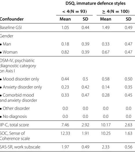
The DSQ was associated with several baseline variables, which were also predictors of the effectiveness measure or the costs. The potential confounders in modelling both effectiveness and costs were gender, ‘psychiatric diagnos-tic category on Axis I’ (DSM IV) [18], ‘IIP-C, total score’ [19], ‘SOC, Sense of Coherence scale’ [20] and ‘SAS-SR, work subscale’ [21] (Table 2). These potential confounders were chosen based both on a priori judgement on psy-chology and on Kendall’s τ with DSQ (p-value smaller than 0.1), and with the AUC or with DCP (p-value smaller than 0.2) (data not shown). Also, we have applied baseline adjustment of the effectiveness by adding the baseline GSI value in the effectiveness model [22]. Due to randomiza-tion, there was no association between therapy group (the
intervention) and DSQ, thus the therapy group was not included in the model.
Models
The basic bootstrap method, which did not adjust for confounders, was compared with two model-based approaches, which adjust for confounders by using regres-sion models. The first model-based method was based on cumulative measures of cost and effectiveness as out-comes, multiple imputation, bootstrap, generalized linear models and frequentist inference. The other method was based on hierarchical regression modelling of GSI and DCP at each MP using the Bayesian inference. These lat-ter methods are described below, and referred to as the frequentist model and the Bayesian model although the models were not restricted to any particular inferential paradigm.
Multiple imputation and bootstrap methods
Multiple imputation [9] of the missing data was per-formed using procedure MI of the Sas System 9.2 [23]. The numerical Markov chain Monte Carlo (MCMC) method of this procedure was chosen because the miss-ing data pattern was not monotonic. The MCMC method, in which the variables of the imputation model were assumed to be multinormally distributed, was applied separately for the DSQ groups. Effectiveness GSI was imputed for the repeated measurement data, and after the imputation the AUC was constructed from the imputed values using equation (4) given in the Appendix. The DCP were log-transformed in the MI. Auxiliary variables were not included in the imputation model due to convergence problems of the EM algorithm, which was used to esti-mate the initial values of imputation model parameters, of procedure MI.
In order to calculate the confidence intervals, the boot-strap method [1] was applied with 500 bootboot-strap samples. Multiple imputation was performed as a single imputation separately for each bootstrap sample [24].
Models for cumulative outcomes with frequentist inference
The observed values of the cumulative costs variable were all positive in this case, and a gamma regression model was therefore applied as the analysis model for the cumulative costs. The AUC was modelled using a linear regression model.
Bayesian model for repeated measurement data
Table 1 Descriptive statistics of outcomes
DSQ, immature defence styles
DSQ<4 (N=93) DSQ≥4 (N=100)
Variable Month Meana SDb NZc NMd Meana SDb NZc NMd
GSI 3 0.85 0.51 7 1.19 0.55 11
GSI 7 0.70 0.48 14 1.08 0.60 19
GSI 9 0.64 0.45 10 1.02 0.63 22
GSI 12 0.65 0.51 13 1.01 0.62 21
AUC of Eff 3–12 0.51 0.31 18 0.8 0.39 30
Costs 0–3 735 251 0 9 832 313 0 15
Costs 3–7 689 309 1 9 802 627 1 15
Costs 7–9 185 259 38 9 234 309 31 19
Costs 9–12 186 345 41 9 238 473 37 20
Cumul. costs 0–12 1818 809 0 12 2131 1323 0 21
Descriptive statistics of the effectiveness and cost outcomes.
aObserved means. bStandard deviations.
cNumber of observations with zero costs. dNumber of observations with missing values.
andk, and zero if no costs had been incurred. A logistic regression model for the binary outcomeCikZwas defined as
PCikZ =1βkZ,Xik
= 1
1+exp{−XikβkZ}
, (1)
Table 2 Descriptive statistics of confounders
DSQ, immature defence styles
<4(N=93) ≥4(N=100)
Confounder Mean SD Mean SD
Baseline GSI 1.05 0.44 1.49 0.49
Gender
•Man 0.18 0.39 0.33 0.47
•Woman 0.82 0.39 0.67 0.47
DSM-IV, psychiatric diagnostic category on Axis I
•Mood disorder only 0.44 0.5 0.58 0.50
•Anxiety disorder only 0.23 0.42 0.14 0.35 •Comorbid mood
and anxiety disorder
0.33 0.47 0.28 0.45
•Other disorder 0.0 0.0 0.0 0.0
•No diagnosis 0.0 0.0 0.0 0.0
IIP-C, total score 7.46 2.92 10.17 2.63
SOC, Sense of Coherence scale
12.33 1.91 10.25 1.63
SAS-SR, work subscale 1.97 0.49 2.33 0.56
Observed means or prevalences, and standard deviations (SD) of the confounders.
where Xik denoted the row vector of the intercept, the confounders, MPkand the binary DSQ group indicator DSQi.βkZwere the corresponding regression coefficients, and exp{βkZ}were the corresponding odds ratios (OR).
The second term of the positive costsCP
ik was defined in a similar fashion. Because the distribution of the pos-itive costs was skewed, the Gamma distribution was applied.
CikP ∼Gammaexp{XikβkP+UiP}τDSQik,τDSQik
. (2)
Random effect UiP was individual. The regression coef-ficients represented the proportional changes in the expected value of the positive outcomes, i.e. a one-unit increase in the value of a covariate corresponded to a exp{β}-fold increase in the expected value. The possible heteroscedasticity was accounted for by allowing disper-sion (inverse of variance-to-mean ratio) parameterτDSQik vary over the DSQ groups and the MPs. Note that if τDSQik = 1 then the expected value of the positive costs was equal to the variance, and if τDSQik > 1 then the variance was smaller.
EffectivenessEikwas modelled by using a linear, hierar-chical model:
Eik =XikβkE+UiE1+UiE2t+ikE, (3)
wheretis the follow-up time at MPk. There was assumed to be an individual linear trend, which was modelled by the random effects partUiE1+UiE2t.
and N(0,σE2,DSQ
ik), respectively. The variance parame-ters σE2,·,· and the dispersion parameters τ·,· were dis-tributed as InverseGamma(3, 1) and Gamma(3, 1) a pri-ori, respectively.
The possible associations between measurement points, and the costs and the effects were accounted for using hierarchical models. The prior distribution for the three random effects were Ui := (Ui1,Ui2,Ui3)T := (UiE1,UiE2, UiP)T ∼ N(0,U) and for the corresponding
covariance matrix U = (σij)i,j ∼ InvW10(I3), where
InvW10 was an abbreviation for the inverse Wishart
dis-tribution with 10 degrees of freedom andI3 the 3×3
identity matrix. Thus the correlation between the ran-dom effects was assumed to be zero a priori, and the costs and effectiveness were therefore assumed to be independent given the observed background information and the random effects. The correlation coefficients of the distribution of the random effects were defined as ρij:=σij/√σiiσjj.
The details of the model specifications, estimation, data augmentation and the model assessment are described below.
Mathematical description of the model
Notations
Let i ∈ {1, 2,. . .,n} =: I index then = 198 subjects andk =1, 2,. . .,K :=5 theKintervention points where the measurements were made. Let timet(1) ≡ 0 denote the baseline andt(K)= 12 the duration of the follow-up in months. As there was some individual variation in the times when the actual measurements were made, letti∗(k) denote the actual kth measurement time when the out-comesCik(DCP during(t∗i(k−1),ti∗(k)]) andEik(GSI) of subjectiwere recorded.
The cumulative cost variable was defined as the sum CCumi := Kk=2Cik. The effectiveness AUC was defined as:
EAUCi := 1 t(K)
K
k=2
Ei,k−1+Eik 2
t(k)−t(k−1). (4)
The incremental cost-effectiveness ratio was defined as
ICER := ¯
CCumDSQ<4− ¯CCumDSQ≥4
¯
EAUCDSQ<4− ¯EDSQAUC≥4, (5)
whereC¯Cum· andE¯·AUCare the DSQ group specific cumu-lative cost and effectiveness AUC means, respectively.
Cumulative outcomes
The model adjustment for controlling confounding was based on the ideas of Lee [6]. The individual predictions, which were based on the parameter values, the covariate
values and the expected value based on the gamma regres-sion model, were:
E CCumi βC,XiC
:=exp{XiCβC} ∀i, (6)
where XiC denotes the row vector of the covariates and βC the corresponding column vector of the regression coefficients.
The analysis model for the effectiveness contains the group DSQi and the confounders. The linear regression model was applied, and the individual predictions were:
E EAUCi βE, σ2,XEi
:=XEiβE ∀i. (7)
The predicted margin [7] was the average of the predic-tions (6):
PMC(xDSQ):= 1 n
n
i=1
E CiCumβC,σ2,XiC,∗
. (8)
In (8)XiC,∗was a modified version of the original covari-ate values. In this modification group variable DSQi was set to valuexDSQ ∈ {DSQ<4, DSQ≥4}for all patients
iand the values of the other covariates remained at their original values. The adjusted difference of groups was difference PMC(DSQ<4)−PMC(DSQ≥4). The predic-tive margins PME(xDSQ)and the difference between the groups PME(DSQ<4) − PME(DSQ≥4) were defined as in (8), but by using the individual predictions defined in (7). The adjusted ICER was calculated by using the predictive margins PME(·)and PMC(·):
ICERPM:= PM
C(DSQ<4)−PMC(DSQ≥4)
PME(DSQ<4)−PME(DSQ≥4). (9)
Repeated measurements
In the Bayesian model, the posterior distribution was pro-portional to the product of the likelihood terms based on equations (1), (2) and (3), the joint density of the ran-dom effects and the joint density of all model parameters (denoted here byθ):
p( θ|data)∝
⎡
⎣
i,k
PCikZβkZ,XikZpCikPXikP,βkP,UiP,τDSQik
⎤
⎦
×
⎡
⎣
i,k
pEik|XikE,βkE,UiE,σE,DSQ2 ik
⎤
⎦
×
i
p(Ui|θ )
×p{θ}.
The predictive distribution of the outcomes for a setIof hypothetical subjectsi∗was defined as
(CZi∗k,CiP∗k,Ei∗k)i∗∈I|data
=
p( θ|data)
i∗
p(Ui∗|θ )
×
k
PCZi∗kβZk,XiZ∗k
p
CiP∗kXiP∗k,βkP,UiP∗,τDSQi∗k
×pEi∗k|XiE∗k,βEk,UiE∗,σE,DSQ2 i∗k
dUi∗dθ.
(11)
Predictive distributions (11) were applied to calculate posterior predictive expectations and quantile points of functionals of
(CiZ∗k,CiP∗k,Ei∗k)i∗∈I,k,
such as PMC(xDSQ)in (8) or the ICERPMin (9).
Estimation
The frequentist regression analyses were performed using the SAS System 9.2 [23] procedures Genmod and Mixed for cumulative costs and AUC, respectively.
The Bayesian analyses were conducted using the Open-Bugs software [13], which applies MCMC methods. The data management and the predictive distributions were handled using the R software [25].
Data augmentation to handle missing data
Predictive distributions (11) were also applied in the data augmentation procedures to handle missing outcome val-ues. The corresponding predictive distribution for the missing baseline covariate valueXij, which belongs to at least one of the covariate vectorsXikZ,XikP orXEik, was
Xij|data∝
p( θ|data)
×pXijθ p(Ui|θ )
k
PCikZβkZ,XikZ
×pCPikXPik,βkP,UiP,τDSQ ik
×pEik|XikE,βkE,UiE,σE,DSQ2 ik
dUidθ.
(12)
The prior distribution for the discretized baseline DSQ was defined as Bernoulli(pDSQ), where the hyperprior for pDSQ was chosen to be Uniform(0, 1). The other base-line covariatesXijhaving missing values were continuous, and they were assigned N(μj, 1/τj) priors with hyperpriors μj ∼ N(0, 1000)andτj ∼ Gamma(2, 1). As the number of missing values in these covariates was small, we chose not to elaborate the prior distributions further.
Convergence checks of MCMC and assessment of model assumptions
Two parallel chains were simulated with 60,000 iterations in addition to 10,000 iterations of burn-in in both chains. The chains were thinned by factor 15 resulting in 4,000 sampled values for both chains. Autocorrelations van-ished quickly, which suggests good convergence (data not shown).
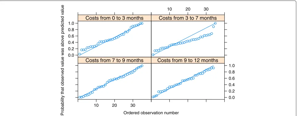
The Bayesian model was assessed using the Q-Q plots of standardised predictive errors (SPE). A total of 40 subjects denoted by setI∗were excluded from the data, and the predictions for these 40 subjects were calculated based on their baseline information and all observed information of the remaining subjects inI∩I∗C. The SPE was defined as
E
Ei∗k−EObsi∗k
σE,
data I∩I∗C
= · · · Ei∗k−EiObs∗k
σE,
pEi∗k|XiE∗k,βkE,UiE∗,σE,2,DSQi∗
×p(Ui∗|θ )p
θ|data{I∩I∗C}dEi∗kdUi∗dθ ∀i∗∈I∗
(13)
where EObsi∗k denotes the observed value of effectiveness GSI. A similar approach for the positive costs CP
ik was
applied.
Results
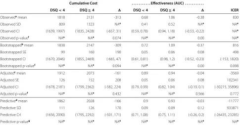
The adjusted absolute differences of the cumulative costs (-161 and -166 based on the frequentist and Bayesian methods, respectively) appeared to be smaller than the unadjusted difference of -309 based on the bootstrap method (Table 3). The unadjusted difference was weakly significantly different from zero (P-value 0.094) whereas the corresponding adjusted difference based on the fre-quentist model was not significant (P-value 0.432). The Bayesian method, which modelled the measurement points separately, appeared to produce slightly lower pre-dictive cumulative cost means than the frequentist predic-tive margins method. The estimates of the difference were close to each others.
The AUC differences for effectiveness were highly significant for the unadjusted bootstrapped difference (-0.38), but the adjusted mean -0.04 based on predictive margins was not significant and close to zero (P-values 0.000 and 0.566, respectively), whereas the predictive mean difference based on the Bayesian inference pro-duced a much smaller difference of -0.03 with credible interval (CrI) (-0.27, 0.20) (Table 3).
Table 3 The observed and model-based estimates
Cumulative Cost . . . Effectiveness (AUC) . . . .
DSQ<4 DSQ≥4 DSQ<4 DSQ≥4 ICER
Observedamean 1818 2131 -313 0.68 1.06 -0.38 830
Observed SD 809 1323 NAe 0.41 0.52 NAe NAe
Observed CI (1639, 1997) (1835, 2428) (-657, 31) (0.59, 0.78) (0.94, 1.18) (-0.53, -0.22) NAe
Observed p-valuef NAe NAe 0.074 NAe NAe 0.00 NAe
Bootstrappedbmean 1838 2147 -309 0.72 1.09 -0.37 816
Bootstrapped SE 99 160 190 0.05 0.06 0.08 498
Bootstrapped CI (1670, 2046) (1855, 2469) (-665, 47) (0.61, 0.81) (0.98, 1.2) (-0.52, -0.23) (-153, 1820)
Bootstrapped p-valuef NAe NAe 0.094 NAe NAe 0.00 0.098
Adjustedcmean 1912 2073 -161 0.89 0.94 -0.04 -3569
Adjusted SE 126 152 208 0.05 0.06 0.08 102341
Adjusted CI (1678, 2181) (1799, 2362) (-582, 224) (0.79, 0.99) (0.82, 1.04) (-0.19, 0.1) (-30215, 35896)
Adjusted p-valuef NAe NAe 0.432 NAe NAe 0.566 0.772
Predictivedmean 1862 2028 -166 0.9 0.93 -0.03 -11777
Predictive SD 111 126 170 0.09 0.09 0.12 933871
Predictive CrI (1656, 2090) (1795, 2292) (-501, 171) (0.71, 1.08) (0.75, 1.11) (-0.26, 0.2) (-26435, 23285)
Predictive p-valueg NAe NAe NAe NAe NAe NAe NAe
The observed and model-based estimates of cumulative costs and effectiveness measured by the area under the curve (AUC).
aThe observed group means, and their standard deviations (SD) and group differences are not adjusted for confounders. 95% confidence intervals (CI) and tests were
based on the t-test.
bThe bootstrapped group means and differences, and their standard errors (SE) are based on multiply imputed and bootstrapped data but unadjusted for confounding. cThe adjusted group means and their differences are based on regression modelling. The rows marked adjusted mean and SE are based on predictive margins,
frequentist inference, bootstrap and multiple imputation.
dThe rows denoted by predictive means and SD are based on the hierarchical Bayesian model, posterior predictive group means and their differences, and the
corresponding SDs and 95% credible intervals (CrI).
eNA corresponds to not applicable results.
fP-values correspond to the null hypothesis “no difference between groups” or “ICER equals zero”. gP-values are generally not sensible in Bayesian inference, thus they are not reported.
posterior expectation of the ICER were not applicable, because the denominator of the ICER (the effectiveness difference) was near zero, in which case the ICER was undefined [2].
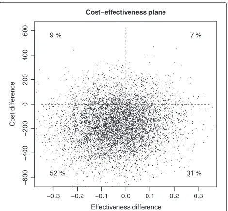
The cost–effectiveness plane shows that in the group where DSQ≥4 both the costs and the symptoms were on a higher level than in the group where DSQ<4 (Figure 1). Due to the large number of parameters in the regres-sion models defined above, which were merely a technical utility as the objective was to adjust the average costs and effectiveness for possible confounding, we focus on a lim-ited number of parameters of the Bayesian model in the following.
There were significant correlations between aver-age levels of individual costs and effectiveness over time (posterior expectation E[ρ1,3|data]= 0.32 and CrI (0.00,0.57)), and the individual slope of effective-ness (E[ρ1,2|data]= −0.17 CrI (-0.33, -0.00)), which cannot be explained by the background informa-tion included in the regression models. The correla-tions between the intercept of positive costs, and the
slope of effectiveness, however, were practically zero (E[ρ1,3|data]= −0.03).
The dispersions of the positive costs showed consid-erable variation over the measurement points, but the residual variances of effectiveness were close to each other (Table 4). During the first measurement interval the pos-itive costs varied relatively little (E[τ·,2|data] were large)
because the majority of patients took the study treat-ments, each of which lasted approximately six months and was covered by the first two measurement intervals. Some patients took auxiliary therapies or other psychiatric treat-ments both during and after the study therapies, which resulted in higher costs, whereas other patients took no auxiliary treatments, which resulted in lower costs. This resulted in greater individual variation during the last measurement interval (E[τ·,5|data] were small).
−0.3 −0.2 −0.1 0.0 0.1 0.2 0.3
−600
−400
−200
0
200
400
600
Cost−effectiveness plane
Effectiveness difference
Cost difference
9 %
52 %
7 %
31 %
Figure 1The cost-effectiveness plane.The Bayesian method was applied to calculate the posterior predictive differences of effectiveness meansE¯AUC
DSQ<4− ¯EDSQAUC≥4and cost means
¯
CCumDSQ<4− ¯CDSQCum≥4.
Discussion
This paper compared the standard bootstrap-based method in a cost-effectiveness analysis with two model-based methods model-based on the frequentist and the Bayesian inferences. The skewed, non-negative distribution of cost variables was analysed using the gamma regression and the two-part models, and model adjustment for potential confounding was performed using the predictive margins
Table 4 Variance parameter estimates
DSQ<4 DSQ≥4
θa E[θ|d]b 95% CIb E[θ|d]b 95% CIb
σ2
E,·,1 0.10 0.07 0.14 0.13 0.09 0.19
σ2
E,·,2 0.09 0.06 0.12 0.12 0.09 0.18
σ2
E,·,3 0.07 0.05 0.11 0.09 0.06 0.13
σE,2·,4 0.10 0.06 0.16 0.17 0.1 0.26
τP,·,1 12.15 8.28 17.19 8.09 5.55 11.37
τP,·,2 6.07 4.06 8.51 3.79 2.61 5.3
τP,·,3 4.12 2.57 6.08 4.67 3.01 6.82
τP,·,4 2.07 1.21 3.13 1.95 1.16 2.91
The parameters controlling the variance of effectiveness and the dispersion of the positive costs in the Bayesian model.
aParametersσ2
E,·,·control the variance of the effectiveness measure, and
parametersτ·,·(inverse of variance-to-mean ratio) the dispersion of the positive costs in the Bayesian model. Parameterθis a generic notation representing one of the parametersσ2
E,·,·orτ·,·.
bThe point estimates are posterior expectationsE[θ|d]and also 95% credible
intervals (CI) are presented
and predictive distributions in the frequentist and the Bayesian inferences, respectively.
The benefit of using the predictive margins method or the predictive distributions of the Bayesian inference to calculate the adjusted averages of costs and effectiveness is that there is that also other link functions than the identity function can be used in regression modeling. For example, Nixon and Thompson [5] applied identity link functions both for gamma distribution of the costs and for the normal distribution of the effectiveness. The average of the covariates over all individuals multiplied by the cor-responding regression coefficients were restricted to zero in order to interpret the intercept terms as the group aver-ages. There is no need to make such restrictions or to stick with the identity link function when using predictive margins or Bayesian predictive distributions. Other link functions, which are commonly used in generalized linear models, can be applied with these methods as well thus avoiding the possibility of negative linear predictors (and predictive values) in case of the gamma distribution.
Both methods based on the regression models could have been applied in the case of repeated measurements by using either frequentist or Bayesian inference. How-ever, the prevalence of zero costs during the first two follow-up periods was very low, thus an application of a logistic regression model and frequentist inference in the two-part model was not plausible. Furthermore, appli-cation of a joint hierarchical model would have been difficult because effectiveness and positive costs were modelled using different families of distributions, nor-mal and gamma distributions, respectively. The Bayesian method avoided the numerical instabilities by using infor-mative prior distributions for the regression coefficients and the missing data values were augmented during the MCMC simulation in a straightforward manner.
Bayesian model averaging [26,27] has been proposed to handle the skewness of cost variables or for the selection of important predictors, respectively, but simultaneous handling of skewness, heteroscedasticity and adjustment for confounding factors can be challenging. We modelled the heteroscedastic residual variance of the cost variables in the case of the repeated measurement data, which allows the model to adapt to the distribution of the costs. The posterior predictive checks suggested that the model fit was good.
The predictive margins approach for the cumulative outcomes was flexible, and the procedure described in this paper can be extended to the case of zero costs and two-part models.
Ordered observation number
Probability that obser
v
ed v
alue w
as abo
v
e
predicted v
a
lue
0.0 0.2 0.4 0.6 0.8
1.0 Measurement at 3 months
10 20 30
Measurement at 7 months
10 20 30
Measurement at 9 months
0.0 0.2 0.4 0.6 0.8 1.0 Measurement at 12 months
Figure 2Q-Q plots of effectiveness outcome GSI.The four measurement points at 3, 7, 9 and 12 months were used.
low during the first seven months of follow-up. There-fore, application of separate random effects for the zero costs (and possible positive correlation with the random effect(s) of the positive costs) was suppressed.
Potential extensions of the model include, for example, using a higher order random effects model for positive costs and adding a random effect to the logistic model of zero costs. These extensions would, however, require more measurements or more individuals. Another exten-sion of the model would be to handle the skewed distri-bution of the effectiveness outcome, especially at the later stages of the follow-up by using, for example, the skewed normal distribution [29].
The patient groups were not defined using (random-ized) intervention groups, which is the case in most
cost-effectiveness analyses, but with the DSQ, which com-plicates the interpretation of the ICER statistic. The DSQ is a rather stable characteristic of a patient, which can-not be altered by a researcher, whereas interventions in general can be altered. The interpretation of the ICER statistic is the change in average costs per one unit in the change of the average effectiveness measured in terms of the AUC. It is also important to bear in mind that in this work large values of the effectiveness outcome GSI correspond to more severe symptoms (less bene-fits) whereas in commonly used effectiveness outcomes such as the quality adjusted life years (QALY) large val-ues correspond to greater benefits. Therefore the usual interpretation of the quadrants of the cost-effectiveness plane[30] is reversed with respect to the vertical axis. In
Ordered observation number
Probability that obser
v
ed v
alue w
as abo
v
e
predicted v
alue
0.0 0.2 0.4 0.6 0.8 1.0
Costs from 0 to 3 months
10 20 30
Costs from 3 to 7 months
10 20 30
Costs from 7 to 9 months
0.0 0.2 0.4 0.6 0.8 1.0 Costs from 9 to 12 months
this case the unadjusted ICER estimates were positive indicating that in the group DSQ¡4 the effectiveness was better and the costs were lower.
Our results allow a decision-maker to assess the impor-tance of patient characteristics such as the DSQ in this study. If a patient in the group DSQ≥4 become similar to a patient in the group DSQ¡4, the cost would decrease by 816 euros (the bootstrapped point estimate) per one unit decrease in the AUC based on the GSI on aver-age. However, the adjusted estimates indicate that not only the effectiveness difference but also the cost differ-ence vanished thus it is not reasonable to present such a standardized estimate of the change in costs as the ICER.
Limitations of the proposed methods are mainly related to the various modelling assumptions, but there are few alternatives to parametric models in order to adjust for confounders. For example, the effectiveness measure was nonnegative, but the model was based on normal-ity assumptions, thus predictive effectiveness values can be negative. The poor performance of the effectiveness model was likely to be due to the skewed distribution, which was not accounted for using a model based on normal distribution. SCL-90-GSI can have only positive values, and the reduction in symptoms caused a con-siderable proportion of observations to lie close to zero. Linearity assumptions or possible interactions were not tested, but could be done in future work.
Conclusion
Our paper demonstrates how to combine several meth-ods for performing cost-effectiveness analyses in obser-vational studies, which are often subject to effects of confounding and missing data. Our results based on regression modelling confirmed that there was a need to adjust for the confounders in this study, thus the stan-dard unadjusted methods based on the bootstrap method, were not adequate. Unadjusted methods showed signifi-cant differences between the groups, but the adjustment for confounders showed no the significant differences thus yielding different conclusions. Not all associations between the costs and effectiveness could not, however, be explained by the observed confounders only, thus the hierarchical model showed clear non-zero correlations between the random effects. The OpenBUGS code is available from the corresponding author upon request.
Competing interests
The authors declare that they have no competing interests.
Authors’ contributions
PK, TH and TM conceived the study. TH developed the methods, conducted the analyses and wrote the manuscript. TM provided expertise in cost-effectiveness analyses. OL and PK provided expertice in psychotherapy. OL, PK ja EV provided the data. EV programmed the SAS macro. All authors read and approved the final manuscript.
Acknowledgements
The work is supported by the Academy of Finland (#138876) and Social Insurance Institution.
Author details
1National Institute of Health and Welfare, Mannerheimintie 166, P.O.Box 30, FIN-00271 Helsinki, Finland.2Social Insurance Institution, Helsinki, Finland.
Received: 2 July 2012 Accepted: 19 March 2013 Published: 28 March 2013
References
1. Efron B:Bootstrap methods: Another look at the jackknife.Ann Stat 1979,7:1–26.
2. Briggs AH, Mooney CZ, Wonderling DE:Constructing confidence intervals for cost-effectiveness ratios: An evaluation of parametric
and non-parametric techniques using Monte Carlo simulation.Stat
Med1999,18:3245–3262.
3. Briggs AH, Wonderling DE, Mooney CZ:Pulling cost-effectiveness analysis up Bby its bootstraps: A non-parametric approach to
confidence interval estimation.Health Econ1997,6:327–340.
4. Polsky D, Glick HA, Willke R, Schulman K:Confidence intervals for
cost-effectiveness ratios: A comparison of four methods.Health Econ
1997,6:243–252.
5. Nixon RM, Thompson SG:Methods for incorporating covariate adjustment, subgroup analysis and between centre differences into
cost-effectiveness evaluations.Health Econ2005,14:1217–1229.
6. Lee J:Covariance adjustment of rates based on the multiple logistic
regression model.J Chronic Dis1981,34(8):415–26.
7. Graubard BI, Korn EL:Predictive Margins with Survey Data.Biometrics 1999,55:652–659.
8. Gelman A, Carlin JB, Stern HS, Rubin DB:Bayesian Data Analysis. London: Chapman & Hall; 1995.
9. Rubin DB:Multiple imputation for nonresponse in surveys. New York: Wiley; 1987.
10. Tanner MA, Wong WH:The calculation of posterior distributions by
data augmentation.J Am Stat Assoc1987,82:528–550.
11. Mullahy J:Much ado about two: Reconsidering retransformation and
the two-part model in health econometrics.J Health Econ1998,
17(3):247–281.
12. Lambert PC, Billingham LJ, Cooper NJ, Sutton AJ, Abrams KR:Estimating the cost-effectiveness of an intervention in a clinical trial when
partial cost information is available: a Bayesian approach.Health
Econ2008,17(1):67–81.
13. Thomas A, O’Hara B, Ligges U, Sturtz S:Making BUGS open.R News2006, 6:12–17.
14. A randomized trial of four forms of the psychotherapy on depressive and anxiety disorders(Knekt P, Lindfors O, eds.) Finland: The Social Insurance Institution; 2004.
15. Andrews G, Pollock C, Stewart G:The determination of defense style
by questionnaire.Arch Gen Psychiatry1989,46:455–460.
16. Maljanen T, Tillman P, Hrknen T, Lindfors O, Laaksonen MA, Haaramo P, Knekt P:The cost-effectiveness of short-term psychodynamic psychotherapy and solution-focused therapy in the treatment of depressive and anxiety disorders during a one-year follow-up.
J Ment Health Policy Econ2012,15:13–23.
17. Derogatis LR, Lipman RS, Covi L:The SCL-90: An outpatient psychiatric
rating scale - Preliminary report.Psychopharmacol Bull1973,9:13–28.
18. American Psychiatric Association:Diagnostic and statistical manual of mental disorders. Washington, DC: American Psychiatric Association, 4th edition; 1994.
19. Horowitz LM, Rosenberg SE, Baer BA, Ureno G, Villasenor VS:The inventory of interpersonal problems: Psychometric properties and
clinical applications.J Consult Clin Psychol1988,56:885–895.
20. Antonovsky A:The structure and properties of the sense of
coherence scale.Soc Sci Med1993,36:725–733.
21. Weissman MM, Bothwell S:Assessment of social adjustment by
patient self-report.Arch Gen Psychiatry1976,33:1111–1115.
22. Manca A, Hawkins N, Sculpher MJ:Estimating mean QALYs in trial-based cost-effectiveness analysis: the importance of
23. SAS/STAT 9.2 User’s Guide 9.2, Cary, NC; 2009.
24. Shao J, Sitter RR:Bootstrap for imputed survey data.J Am Stat Assoc 1996,91:1278–1288.
25. R Development CoreTeam:R: A Language and Environment for Statistical Computing. R Foundation for Statistical Computing. Austria: Vienna; 2011. [http://www.R-project.org/]. [ISBN 3–900051-07–0]
26. Conigliani C, Tancredi A:Semi-parametric modelling for costs of
health care technologies.Stat Med2005,24(20):3171–3184.
27. Negrin MA, Vazquez-Polo FJ:Incorporating model uncertainty in cost-effectiveness analysis: A Bayesian model averaging approach.
J Health Econ2008,27(5):1250–1259.
28. Olsen MK, Schafer JL:A two-part random-effects model for
semicontinuous longitudinal data.J Am Stat Assoc2001,
96(454):730–745.
29. O’Hagan T, Leonhard T:Bayes estimation subject to uncertainty about
parameter constraints.Biometrika1976,63:201–202.
30. Cohen DJ, Reynolds MR:Interpreting the results of cost-effectiveness
studies.J Am Coll Cardiol2008,52(25):2119–2126.
doi:10.1186/2191-1991-3-8
Cite this article as:H¨ark¨anenet al.:Confounding and missing data in
cost-effectiveness analysis: comparing different methods.Health Economics Review20133:8.
Submit your manuscript to a
journal and benefi t from:
7Convenient online submission
7Rigorous peer review
7Immediate publication on acceptance
7Open access: articles freely available online
7High visibility within the fi eld
7Retaining the copyright to your article