CSOLNP: Numerical Optimization Engine for Solving Non-linearly Constrained Problems

(1)

Volume 20 Number 4 pp. 290–297 C The Author(s) 2017 doi:10.1017/thg.2017.28

CSOLNP: Numerical Optimization Engine for

Solving Non-linearly Constrained Problems

Mahsa Zahery,1_{Hermine H. Maes,}2_{and Michael C. Neale}2

1_{Department of Computer Science, Virginia Commonwealth University, Richmond, Virginia, USA} 2_{Department of Psychiatry, Virginia Commonwealth University, Richmond, Virginia, USA}

We introduce the optimizer CSOLNP, which is a C++implementation of the R package RSOLNP (Ghalanos & Theussl, 2012, Rsolnp: General non-linear optimization using augmented Lagrange multiplier method. R package version, 1) alongside some improvements. CSOLNP solves non-linearly constrained optimization problems using a Sequential Quadratic Programming (SQP) algorithm. CSOLNP, NPSOL (a very popular implementation of SQP method in FORTRAN (Gill et al., 1986, User’s guide for NPSOL (version 4.0): A For-tran package for nonlinear programming (No. SOL-86-2). Stanford, CA: Stanford University Systems Opti-mization Laboratory), and SLSQP (another SQP implementation available as part of the NLOPT collection (Johnson, 2014, The NLopt nonlinear-optimization package. Retrieved from http://ab-initio.mit.edu/nlopt)) are three optimizers available in OpenMx package. These optimizers are compared in terms of runtimes, final objective values, and memory consumption. A Monte Carlo analysis of the performance of the optimiz-ers was performed on ordinal and continuous models with five variables and one or two factors. While the relative difference between the objective values is less than 0.5%, CSOLNP is in general faster than NPSOL and SLSQP for ordinal analysis. As for continuous data, none of the optimizers performs consistently faster than the others. In terms of memory usage, we used Valgrind’s heap profiler tool, called Massif, on one-factor threshold models. CSOLNP and NPSOL consume the same amount of memory, while SLSQP uses 71 MB more memory than the other two optimizers.

Keywords:OpenMx, non-linear programming, sequential quadratic programming, RSOLNP, NPSOL, SLSQP

In all structural equation modeling (SEM) techniques, al-ternative models are designed to test a hypothesis of in-terest. These models are fitted to data to find the best set of parameters that minimizes the difference between mod-els and data. To minimize the misfit between the modmod-els and data, SEM needs optimization, which unfortunately is not an exact science. Optimization problems have differ-ent ‘landscapes’ to search, and the best search algorithm de-pends somewhat on the features of the landscape. OpenMx currently offers three optimizers, which differ in their abil-ities to find the solution. A goal of this article is to help the applied researcher select the right optimizer for the problem at hand. We focus on full information maximum likelihood (ML) of ordinal data because this is a complex problem that is subject to local minima.

CSOLNP, short for C++-based optimizer forSolving

NonlinearPrograms, is one of the optimizers available in the OpenMx package (Boker et al.,2011; Neale et al.,2016). OpenMx is an open-source software package licensed un-der Apache 2.0, which is widely used for SEM and other statistical modeling. It runs inside R, and provides model

specification in both path style and matrix style, as well as optimizers for handling non-linear equality and inequal-ity constraints. NPSOL (short for Nonlinear Programming at Systems Optimization Laboratory at Stanford; Gill et al., 1986) was the only available optimizer in Mx or OpenMx since the early 1990s. Recently, SLSQP (short for Sequential Least-Squares Quadratic Programming) from NLOPT col-lection (Johnson,2014) has been added to OpenMx. Here, we compare CSOLNP to NPSOL and SLSQP within the OpenMx package. Similar to NPSOL and SLSQP, CSOLNP solves non-linear problems by applying the SQP method to a linearly constrained Augmented Lagrangian objec-tive function. While optimizers use similar algorithms,

received 7 December 2016; accepted 13 April 2017. First published online 24 May 2017.

(2)

the implementations are different. Details of the CSOLNP optimizer will be explained in the methods section. The rest of this section provides a general description of the CSOLNP optimizer.

CSOLNP solves non-linear problems of the form:

argmin f(x) subject to :

g(x)=0

lh≤h(x)≤uh

lx≤x≤ux

where

f(x) :Rn_→_R_{is the objective function (}_n_{is the}

num-ber of free variables),

g(x) :Rn_→_Rme_{are the equality constraint functions} (meis the number of equality constraints),

h(x) :Rn_→_Rmi _{are the inequality constraint} func-tions (miis the number of inequality constraints), lh,uhare the lower and upper bounds for inequalities,

andlx,uxare the bounds for free variables.

CSOLNP is an iterative algorithm that solves a QP sub-problem at each major iteration. QP is a special case of non-linear programming optimization where the objective function is quadratic and the constraints are linear. Each major iteration starts by solving a linearly constrained prob-lem with an augmented Lagrangian objective function of the following form:

argmin f(x)−yk_g₍_x₎₊ρ

2 g(x) 2

subject to :

Jk₍_x₋_xk₎_{= −}_g₍_xk₎

lx≤x≤ux

The inequality constraints are converted to equality con-straints by adding slack variables. The superscriptkdenotes the iteration number, andJk_{is the Jacobian matrix:}

Jk= ∂g

∂x|xk

The original objective function is converted to an aug-mented Lagrangian function, which incorporates a penalty term (ρ), as well as a Lagrange multiplier term (y). The penalty term is used to penalize the objective function if the current point estimation is violating the constraints, while the Lagrange multiplier is used to reduce the computational cost imposed by updating the penalty term at each iteration. The augmented Lagrangian objective function plays the role of a merit function measuring the quality of each iter-ation for finding a better point estimate.

The augmented Lagrangian objective function is a very common choice for a merit function (Biegler et al.,2003). This method does not have the drawback of penalty meth-ods in terms of having to face an ill-conditioned uncon-strained problem with huge gradients. For penalty meth-ods, the penalty parameter is increased at each iteration to ensure that the unsatisfied constraints are penalized more

severely, which eventually helps the optimizer stay close to a feasible region. Hence, optimization is achieved when the penalty parameter is increased to infinity while the term

g(x)2_{is close to zero, suggesting that no constraints are} violated. But increasing the penalty parameter to infinity can result in increasing the condition number of the prob-lem to infinity as the algorithm proceeds. Condition num-ber is the sensitivity of the output of a system with respect to small errors in the input. Hence, a large condition num-ber implies that small changes in the input data can make drastic changes in the solution of a system. A system with a large condition number is called ill-conditioned and its solution is not reliable. The augmented Lagrangian method uses a Lagrange multiplier term that avoids ill-conditioning by stopping the penalty parameter from approaching infin-ity (Wright & Nocedal,1999).

After converting the problem to an augmented La-grangian function with linearized constraints, CSOLNP continues with a feasibility check of the current point. The region that is bounded by the constraints of the problem is called the feasible region. Any point in this region is called feasible. If the current point is feasible, CSOLNP continues with finding an optimal solution in the feasible region. Oth-erwise, a phase 1 Linear Programming (LP) procedure is applied to find a feasible point.

A two-phase LP technique approaches the optimal so-lution of a system in two phases, feasibility seeking and optimality seeking. In phase 1, an auxiliary problem is constructed by introducing artificial variables. Artificial variables do not have any physical meaning. They are only introduced to the problem to find a feasible solution.

In phase 1, one artificial variable is added for each≥ and=constraints. The original problem is then replaced with the sum of these artificial variables. Since artificial variables should not become part of an optimal solution to the original problem, they have to be zero at the feasible so-lution, and subsequently the sum of them should be equal to zero. Hence, the goal is to minimize the new objective func-tion subject to the constraints of the original problem. If the minimum objective value is zero, then the original problem has a feasible solution. This feasible solution is used as the starting point for phase 2, where the original objective func-tion is minimized for finding the optimal solufunc-tion.

After finding a feasible point, a QP sub-problem is solved to find the search direction. The idea behind using a QP sub-problem is that it can reflect the non-linearity of the original problem in its quadratic objective function. Also, the linear constraints make the original problem easy to solve. An obvious choice of a QP sub-problem would have the following format:

argmin ∇f(xk₎T₍_x₋_xk₎₊ 1

2(x−xk)TH(x−xk) subject to :

∇g(xk₎₍_x₋_xk₎₊_g₍_xk₎₌₀

(3)

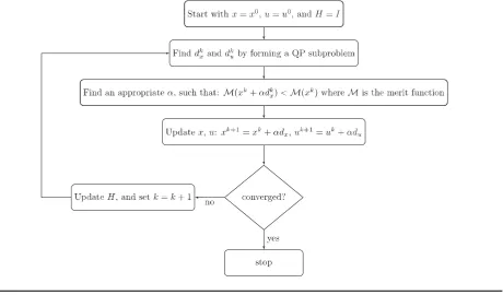
FIGURE 1

A flowchart of CSOLNP’s algorithm. Starting with initial set of free variablesx0_{, and Lagrange multipliers}_u0_{, the search directions}_dk x

anddk

uare found by solving a QP sub-problem. Finding an appropriate step lengthα, CSOLNP updates the free variables and Lagrange

multipliers. If the difference between the current objective value and the previous objective value is less than the optimality tolerance, the point estimates are considered to be converged, and CSOLNP reports the final set of free variables as the optimum. Otherwise, the Hessian matrixHis updated, and CSOLNP continues with the next iteration.

where

∇denotes the first derivative,

Tdenotes transpose, and

His an approximation to the hessian of the Lagrangian of the objective functionL(xk_,_uk_).

Here, the objective function is obtained by the quadratic approximation of the original objective function at the cur-rent estimatexk_{, and the constraints are the linear} approxi-mations of the actual constraints at the same point estimate. After the directiondk

x=x−xk is found, CSOLNP pro-ceeds by finding a step length (α) that satisfies all the con-straints and provides sufficient decrease in the augmented Lagrangian merit function. The next iteration starts from the new point estimatexk+1₌_xk₊_α_dk

x.

The solution of each QP sub-problem is a search direc-tion toward a better point estimate. Eventually, after each iteration of SQP algorithm, a better approximation,xk+1_, is constructed. The sequence of these approximations are hoped to converge to a solution for the original constrained non-linear problem. A flowchart of CSOLNP algorithm is provided inFigure 1.

In the methods section, CSOLNP’s algorithm will be de-tailed. What occurs at each iteration of both the SQP al-gorithm and the QP sub-problem will be explained. Next, the choice of step lengthαand the convergence criteria will

be discussed. Finally, a new feature added to the optimizer for handling inequality constraints when not satisfied at the starting point is discussed.

Methods

CSOLNP Algorithm

The procedure through which CSOLNP finds the solution of a non-linear problem is as follows:

Initialization.Given the objective function and the con-straints, CSOLNP starts with setting the following control parameters. All of these parameters except the penalty pa-rameter can be user defined. The default values for these parameters are provided in parentheses:

1. maximum number of major iterations (iterations of the SQP algorithm=400);

2. maximum number of minor iterations (iterations of the QP subproblem=800);

3. penalty parameter (ρ=1);

4. perturbation parameterδin finite differences method for finding the numerical gradient (=1e-7);

5. tolerance on feasibility and optimality (=1e-9).

(4)

An augmented parameter vector containing the inequal-ity evaluations at the starting point as well as free vari-ables’ starting values is created. The corresponding Hessian matrix is initialized with the identity matrix for the first iteration.

Iterations of the SQP algorithm (major iterations).

The first major iteration of the SQP algorithm starts by scaling the objective value, the constraints and the free variables.

The gradients and the Jacobian are calculated using the forward difference method. The default value for the per-turbation parameter (δ) is 1e-7.

The candidate point is checked for feasibility. If it is not feasible, a phase 1 LP procedure is performed to start the QP algorithm with a feasible point. CSOLNP implements phase 1 with a combination of Affine Scaling Method and Gradient Projection Method in the sense that the feasibility direction is found using the Affine Scaling Method, while the step to move along this direction is found using the Gra-dient Projection Method.

The Affine Scaling Method is a simplified variant of Kar-markar’s algorithm (Karmarkar,1984). The basic idea be-hind this method is to start with a point lying in the in-terior (inside the boundaries) of the feasible region, and move in the direction of negative gradient descent to re-duce (for minimization) the objective value at the fastest possible rate. Moving toward the direction of negative gra-dient descent, we might fall out of the feasible region. To have more space for reducing the objective value before hit-ting the boundaries of the feasible region, the Affine Scal-ing Method changes the coordinates of the feasible point to be placed at equal distance from the boundaries. In other words, it transforms the feasible region to place the cur-rent point at its center. So, for a standard LP problem of the form:

mincT_x subject to :

Ax=b x≥0

whereAis of sizembyn;xandcare vectors ofnelements andbis a vector ofmelements, the Affine Scaling Method aims at moving in the direction of negative gradient of the objective function which is −c. Moving in this direction, the objective value is reduced, but we may violateAx=b. To avoid this,−cis projected into the null space of matrix

Awhich is the set of all feasible direction vectors. This pro-jection is

P=I−AT(AAT)−1A

Hence, the projected gradient isPcand the feasible di-rection would be−Pc. The last part of the Affine Scaling Method is to have the projected gradient near the center of the feasible region. This way, there is more room for fur-ther iterations of the algorithm. For this purpose, the

cur-rent pointxis rescaled to the pointX =D−1_x_{, where}_D_is a diagonal matrix of the elements of vectorx. This changes the LP problem to minimizingcT_DX_{, subject to}_ADX₌_b andx≥0. Subsequently, the projection becomesP=I−

˜

AT_{( ˜}_A_A_˜T₎−1_A_˜_{, where ˜}_A₌_AD_{. So, the projected gradient is} Pc˜with ˜cbeingDc. The new point is thenxk+1₌_xk₋_α_P_c_˜_, whereαis the step length which is obtained by the Gradient Projection Method as the following:

α=

_xi₋_ui

vi , if vi<0 xi−li

vi , if vi>0

wherevis the search direction obtained by the Affine Scal-ing Method, andli,uiare respectively the lower and upper bounds forxi.

The objective value and the constraints are re-evaluated in case the starting point has been replaced with a feasible one. The merit function is also evaluated at the candidate point.

Iterations of the QP algorithm (minor iterations).The gradient of the merit function is calculated (using the for-ward difference method). If this is the first iteration of the QP algorithm, the algorithm considers the identity ma-trix as the Hessian approximation. Otherwise, a quasi-Newton approximation to the Hessian of the Lagrangian is calculated. In general, when the Hessian of the prob-lem is dense, the quasi-Newton approximation can be a better choice, as it saves the computation time per it-eration. CSOLNP uses the Broyden–Fletcher–Goldfarb– Shanno (BFGS) quasi-Newton approximation to the Hes-sian at each iteration of the QP algorithm:

Hk+1=Hk+ 1 yT_dyy

T₋HddTH

dT_Hd

WhereHis the Hessian matrix,disxk+1₋_xk_{, and}_y_{is the} change in the gradient:gk+1₋_gk_.

Finding the search direction.The QP algorithm finds the search direction using the Newton method. The search direction is obtained by Cholesky factorization of the Hes-sian matrix:Hk_dk_{= −}_gk_.

The Newton algorithm is considered to converge when all the constraints (formulae 1 and 2) and free variables’ bounds (formula 3) are satisfied.

Finding steplengthα.After finding the search direction, a new temporary point is approximated: xk+1₌_xk₊_dk_. This point is not yet considered a new estimate for the next iteration. It is necessary to figure out the length of the step to move along the direction from the current point toward this temporary point.

(5)

Finding the next point estimate.Having the search di-rection and the step size, CSOLNP finds the next point es-timate:xk+1=xk+αdk, and a new iteration of the QP al-gorithm starts.

Convergence of the QP algorithm and restoring the results.The QP algorithm stops if the difference between the objective value at the current iteration of the QP algo-rithm and the previous iteration is less than the optimality tolerance.

The vector of free variables, the Hessian matrix, as well as the objective value and the Lagrange multipliers (in case there are constraints) are updated, and a new iteration of the SQP algorithm (major iteration) is started.

Convergence of the SQP algorithm. The problem is converged when the difference between the current objec-tive value and the previous objecobjec-tive value is less than the optimality tolerance. Additionally, the constraints are satis-fied to within the feasibility tolerance.

Improvements of CSOLNP Over RSOLNP

Although RSOLNP can find the solution when the inequal-ity constraints are not satisfied at the starting point, there are cases where it fails to find the correct optimum. We have overcome this difficulty in CSOLNP by adding a new fea-ture. For cases where the inequality constraints are not satis-fied initially, CSOLNP replaces the objective function with the sum of violated inequalities, and optimizes the param-eters with respect to this new objective function. The opti-mum will then be used as the starting point for the original problem (original objective function). This feature has en-hanced the performance of CSOLNP over RSOLNP, in the sense that models failing with RSOLNP now run success-fully with CSOLNP (the results are validated by the other two optimizers).

Application

We have compared the performances of CSOLNP, NPSOL, and SLSQP on factor models with ordinal and continuous variables. A brief description of factor models and how or-dinal variables are measured with such models is presented in the remainder of this section.

Factor analysis is a statistical method assuming a set of unobserved, underlying factors (latent variables) are re-sponsible for variation among a set of observed variables. The regression of an observed variable on a factor is inter-preted as factor loading. Consideringpobserved variables,

mfactors, andnsubjects, the factor model can be written as

Yi j=biXj+Ei j

wherei=1, …,pvariables andj=1, …,nsubjects.Yi js represent observed variables for each subject.Xjare factor scores, which are values of each factor for each of the sub-jectsjin the sample.bis are factor loadings.Ei jis unique for each observed variable, and explains the variability beyond

that explained by common factors. Factor loadings are esti-mated as

YY =BPB+E

where_yyis ap×pcovariance matrix of observed vari-ables,Bis ap×mmatrix of factor loadings,Pis anm×m

covariance matrix of the common factors, andEis ap×p

matrix of specific variances.

In confirmatory factor models, a hypothesized factor model is tested to find whether the sample data supports the model. There are several estimation procedures to find the model parameters. One is ML, which evaluates the goodness of fit of the hypothesized model to the sample data by estimating the matrix of factor loadings. Model estition is considered successful if the original covariance ma-trix can be reproduced from the estimated factor loadings. If it cannot be reproduced, then the hypothesized model may have not been correctly specified.

Maximum likelihood estimation (MLE) assumes multi-variate normality (mvn) of residuals of a model with con-tinuous measures. Behavioral data are often binary (yes/no responses) or ordinal (none/some/a lot), which are inher-ently less accurate than continuous measures. A common approach with binary/ordinal data is to assume that there is a latent, normally distributed continuous variable underly-ing each binary/ordinal symptom or item. For example, in substance use behavior, sensitivity to the rewarding experi-ence of drug use may form part of the underlying propensity to use substances frequently.

Such liability is typically thought of as being due to the additive effects of a large number of factors each of small effect, which the central limit theorem predicts will gen-erate a normal distribution of liability. Thresholds on this liability distribution delimit binary or ordinal response cat-egories. For binary data, yes responses are observed above a threshold, while no responses are observed below that. For ordinal data, the number of thresholds is one fewer than the number of categories in the data. For example, sub-jects with scores below the first threshold have observed value of none. Subjects with scores in between the first and second thresholds have observed value of some, and those with scores above the second threshold have observed value of a lot.

(6)

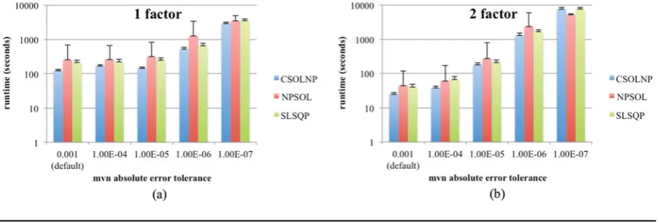
FIGURE 2

(Colour online) Runtimes of CSOLNP, NPSOL, and SLSQP in logarithmic scale for threshold models with (a) five variables and one factor, and (b) five variables and two factors for a sample of size of 1,000. Runtimes are averaged over 250 different runs.

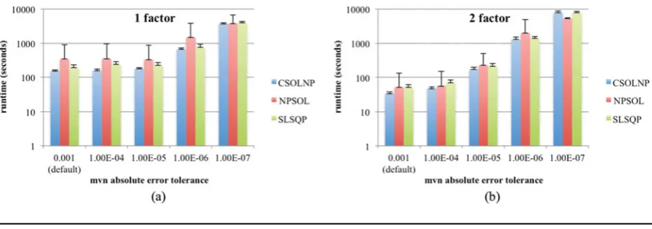
FIGURE 3

the performances of CSOLNP, NPSOL, and SLSQP. Other varying elements in our simulations are the number of la-tent variables (factors) and the sample sizes. The models are run with 1 and 2 factors on datasets of size 1,000, 10,000, and 20,000 samples. The results section illustrates the per-formances of the three optimizers on different threshold and continuous models averaged over 250 simulations.

Results and Discussion

We compared the performances of CSOLNP, NPSOL, and SLSQP on threshold models, as well as continuous models with five variables and one to two factors.

Having five variables and one or two factors, the parame-ters for equationYY =BPB+Eare defined as the follow-ing: matrixBis a 5×2 matrix of factor loadings. The start-ing values are set to 0.2 for all factor loadstart-ings. MatrixPis an identity matrix in our models. MatrixEis a 5×5 matrix of residual variances obtained by the equationE=1−B∗B. Finally, the model’s expected covariance is calculated. At each iteration of the optimization algorithm, the difference

between the model’s expected covariance and the observed covariance is minimized to find the model that best fits the data.

Comparing Runtimes of Optimizers

For threshold models, the performances were compared with respect to runtime of the optimizers when mvn in-tegration absolute error tolerance is reduced from 1e-3 to 1e-7. Figures 2–4 illustrate the runtimes in logarithmic scale for threshold models with one and two factors on sam-ples of 1,000, 10,000, and 20,000 sizes, respectively. The re-sults are averaged over 250 simulations. The error bars show the standard deviation of each optimizer’s runtime obtained from 250 different runs. We also compared the final objec-tive values at which the three optimizers stop. The relaobjec-tive difference between the final objective values are less than 0.5%, and hence not shown.

(7)

FIGURE 4

FIGURE 5

(Colour online) Runtimes of CSOLNP, NPSOL, and SLSQP in logarithmic scale for continuous models with (a) five variables and one factor, and (b) five variables and two factors for samples of sizes 1,000, 10,000, and 20,000. Runtimes are averaged over 250 different runs.

absolute error tolerance dictates the accuracy of numerical integration. Since there is no closed form solution for the integration of the mvn distribution, it is carried out numer-ically to a particular degree of numerical precision. How-ever, the more precise the integral calculation, the longer it takes. NPSOL is in general the slowest optimizer, except when the absolute error tolerance is 1e-7. For other values of absolute error tolerance, CSOLNP is faster than the other optimizers.

Figure 5 illustrates runtime of the three optimizers in logarithmic scale for continuous models with one and two factors on samples of 1,000, 10,000, and 20,000 sizes, respec-tively. The results are averaged over 250 simulations. Since mvn integration is not required to calculate the likelihood for continuous data, the mvn parameter value is irrelevant. The final objective values are almost identical for the three optimizers and hence not shown.

The runtimes differ little between optimizers for contin-uous data analysis. None of the optimizers performs consis-tently faster than the others for such models.

Comparing Memory Usage of Optimizers

Valgrind is a memory management tool suite used for de-bugging and profiling. We used Massif, a heap profiler tool available in Valgrind, to compare memory consumption of the optimizers. We ran the one-factor, five-variate model with default value for mvn absolute error tolerance (1e-3) under Massif for all three optimizers. CSOLNP and NPSOL reach to peak memory of 417.8 MB, while SLSQP’s peak is at 489.8 MB. SLSQP consumes about 71 MB memory more than CSOLNP and NPSOL.

(8)

inconsistent and has the largest standard deviations in most of the cases. In terms of memory management, CSOLNP uses less amount of memory in comparison with SLSQP or the same amount when compared with NPSOL. All the above points make CSOLNP the preferred OpenMx optimizer for threshold model analysis.

The simple factor model is expected to have performance similar to any analysis of multivariate data, such as the classical twin study. Thus, we can recommend CSOLNP as the preferred choice for ordinal data from twins, although it should be noted that multidimensional integration be-comes intractable computationally beyond a total of about 20 variables, that is, 10 variables per twin.

References

Biegler, L. T., Ghattas, O., Heinkenschloss, M., & Bloemen Waanders, B. (2003). Large-scale PDE-constrained opti-mization: An introduction.Large-Scale PDE-Constrained Optimization,30, 3–13.

Boker, S., Neale, M., Maes, H., Wilde, M., Spiegel, M., Brick, T., … Mehta, P. (2011). OpenMx: An open source extended structural equation modeling framework.Psychometrika, 76, 306–317.

Genz, A. (1992). Numerical computation of multivariate nor-mal probabilities.Journal of Computational and Graphical Statistics,1, 141–149.

Ghalanos, A., & Theussl, S. (2012). Rsolnp: General non-linear optimization using augmented Lagrange multiplier method. R package version, 1. Retrieved from http:// CRAN.R-project.org/package=Rsolnp

Gill, P. E., Murray, W., Saunders, M. A., & Wright, M. H. (1986). User’s guide for NPSOL (version 4.0): A For-tran package for nonlinear programming (No. SOL-86-2). Stanford, CA: Stanford University Systems Optimization Laboratory.

Johnson, S. G. (2014). The NLopt nonlinear-optimization package. Retrieved fromhttp://ab-initio.mit.edu/nlopt. Karmarkar, N. (1984). A new polynomial-time algorithm for

linear programming. Proceedings of the Sixteenth Annual ACM Symposium on Theory of Computing, pp. 302–311. New York, NY: ACM Special Interest Group on Algorithms and Computation Theory.

Neale, M. C., Hunter, M. D., Pritikin, J. N., Zahery, M., Brick, T. R., Kirkpatrick, R. M., …Boker, S. M. (2016). OpenMx 2.0: Extended structural equation and statistical modeling. Psychometrika,81, 535–549.