http://Business.ExpertJournals.com
Linear and Non-Linear Regression: Powerful and
Very Important Forecasting Methods
Athanasios VASILOPOULOS
*St. John’s University, United States
Regression Analysis is at the center of almost every Forecasting technique, yet few people are comfortable with the Regression methodology. We hope to improve the level of comfort with this article. In this article we briefly discuss the theory behind the methodology and then outline a step-by-step procedure, which will allow almost everyone to construct a Regression Forecasting function for both the linear and some non-linear cases. Also discussed, in addition to the model construction mentioned above, is model testing (to establish significance) and the procedure by which the Final Regression equation is derived and retained to be used as the Forecasting equation. Hand solutions are derived for some small-sample problems (for both the linear and non-linear cases) and their solutions are compared to the MINITAB-derived solutions to establish confidence in the statistical tool, which can be used exclusively for larger problems.
Keywords: Linear Regression, Non-Linear Regression, Best-Fitting Model, Forecasting
JEL Classification: M10
1. Introduction and Model Estimation for the Linear Model
Regression analysis, in which an equation is derived that connects the value of one dependent variable (Y) to the values of one independent variable X (linear model and some non-linear models), starts with a given bivariate data set and uses the Least Squares Method to assign the best possible values to the unknown multipliers found in the models we wish to estimate. The bivariate data, used to estimate the linear model and some non-linear models, consists of n ordered pairs of values:
(x
1, y
1), (x
2, y
2),..., (x
n, y
n)
The linear model we wish to estimate, using the given data, is:
= + (1)
*
Corresponding Author:
Athanasios Vasilopoulos, Ph.D., St. John’s University, The Peter J. Tobin College of Business, CIS/DS Department, 8000 Utopia Parkway Jamaica, N.Y. 11439
Article History:
Received 2 November 2015 | Accepted 23 November 2015 | Available Online 19 December 2015 Cite Reference:
Vasilopoulos, A., 2015. Linear and Non-Linear Regression: Powerful and Very Important Forecasting Methods. Expert Journal of Business and
Expert Journal of Business and Management, 3(2), pp.205-228
while the non-linear models of interest are given by
= (Exponential Model) (2)
= (Power Model) (3)
and
= + + (Quadratic Model) (4)
To estimate model (1) we use the Least Squares Methodology, which calls for the formation of the quadratic function:
, = ∑!" − = ∑!" − 2 ∑!" − 2 ∑!" + 2 ∑!" + ∑!" (5)
To derive the “normal” equations for the linear model from which the values of a and b of the linear model are obtained, we take the partial derivative of Q(a,b) of equation (5) with respect to a and b, set each equal to zero, and then simplify:
The result is:
∂
Q(a, b)
∂
a
=−
2
i=1y
in
∑
+
2b
x
ii=1
n
∑
+
2a n
(6)
and
∂
Q(a, b)
∂
b
=−
2
i=1X
iy
in
∑
+
2a
x
ii=1
n
∑
+
2b
x
i2i=1
n
∑
(7)
When (6) and (7) are set equal to zero and simplified, we obtain the “Normal” equations for the linear model:
n a
+
b
x
ii=1
n
∑
=
y
ii=1
n
∑
(8)
a
x
ii=1
n
∑
+
b
x
i2i=1
n
∑
=
x
iy
ii=1
n
∑
(9)
The only unknowns in equation (8) and (9) are a and b and they should be solved for them simultaneously, thus deriving (or estimating) the linear model. This is so because all the other values of equations (8) and (9) come from the given data, where:
n = number of ordered pairs (
x
i, y
i)x
ii=1
n
∑
=
x
1+
x
2+
...
+
x
n= sum of the x valuesy
ii=1
n
∑
=
y
1+
y
2+
...
+
y
n= sum of the y valuesx
i2i=1
n
∑
=
x
12+
x
22
+
...
+
x
n
2
= sum of the given x values, which are first squared
x
iy
ii=1
n
∑
=
x
1y
1+
x
2y
2+
...
+
x
ny
n= sum of the products of the xi and yi values in each ordered pair.Optimization methodology of Differential Calculus for functions of 2 independent variables.
To complete the Estimation of the Linear model we need to find the standard deviation for a, σ(a), and b, σ(b), which are needed for testing of the significance of the model. The standard deviations, σ(a), and σ(b), are given by:
σ
(a)
=
σ
ˆ
n
x
i2i=1
n
∑
(x
i−
x )
2i=1
n
∑
1/2
=
σ
ˆ
n
x
i2i=1
n
∑
x
i2i=1
n
∑
−
x
ii=1
n
∑
2
n
1/2
(10)
and
σ
(b)
=
σ
ˆ
(x
i−
x )
2i=1
n
∑
1/2
, (11)
where:
ˆ
σ
=
y
i2i=1
n
∑
−
a
y
ii=1
n
∑
−
b
x
iy
ii=1
n
∑
n
−
2
1/2
(12)
The a and b in equation (12) come from the solution of equations (8) and (9) while
y
i2i=1
n
∑
,
y
ii=1
n
∑
, and
x
iy
ii=1
n
∑
come directly from the given bivariate data.
2. Model Testing
Now that our model of interest has been estimated, we need to test for the significance of the terms found in the estimated model. This is very important because the results of this testing will determine the final equation which will be retained and used for Forecasting purposes.
Testing of the linear model consists of the following steps:
2.1. Testing for the significance of each term separately
Here we test the hypotheses: 1. H0: β = 0 vs H1: β≠ 0, and
2. H0: α = 0 vs H1: α≠ 0, based on our knowledge of b, σ(b), a, and σ(a).
If n ≥ 30, we calculate
Z
b*=
b
σ
(b)
andZ
a*=
a
σ
(a)
and compare each to Zα/2 (where Zα/2 is a value obtained from the standard Normal Table when α, or
Expert Journal of Business and Management, 3(2), pp.205-228
For example if α = 0.05, Zα/2 = Z0.025 = 1.96; if α = 0.10, Zα/2 = Z0.05 = 1.645; if α = 0.02, Zα/2 = Z0.01
= 2.33 and if α = 0.01, Zα/2 = Z0.005 = 2.58).
If Z*
b > Zα/2 (or Z*b < -Zα/2), the hypothesis H0: β = 0 is rejected and we conclude that β≠ 0 and the
term bx (in the estimated model ŷ=a+bx) is important for the calculation of the value of y. Similarly, if Z* a >
Zα/2 (or Z*a < -Zα/2), H0: α = 0 is rejected, and we conclude that the linear equation ŷ=a+bx does not go
through the origin.
If n < 30, we calculate
t
b*=
b
σ
(b)
andt
a*=
a
σ
(b)
and compare each to tn-2(α/2), for a given α value, where tn-2(α/2) is obtained from the t-distribution
table, with the same interpretation for H0: β = 0 and H0: α = 0 as above.
But, instead of hypothesis testing, we can construct Confidence Intervals for β and α using the equations:
$ − %∝⁄ ( ≤ * ≤ + %∝⁄ ( = 1−∝ (13)
and, if n ≥ 30,
$ − %∝⁄ ( ≤∝≤ + %∝⁄ ( = 1−∝ (14)
or
$ − , - ∝⁄ ( ≤ * ≤ + , - ∝⁄ ( = 1−∝ (15)
and, if n < 30,
$ − , - ∝⁄ ( ≤∝≤ + , - ∝⁄ ( = 1−∝ (16)
If the hypothesized values: β = 0 falls inside the Confidence Intervals given by equations (13) or (15), or α = 0 falls inside the Confidence Intervals given by equations (14) or (16), the corresponding hypotheses H0: β = 0 and H0: α = 0 are not rejected and we conclude that β = 0 (and b = 0 and the term bx is
not important for the calculation of y) and α = 0 (i.e. a = 0 and the line goes through zero). If for a given data set, we performed the above-discussed tests, we will obtain one of 4 possible conclusions:
A) H0: β = 0 and H0: α = 0 are both rejected; Therefore β≠ 0, and α≠ 0, and both the terms a and bx
are important to the calculation of y. In this case the final equation is ŷ=a+bx, with both terms staying in the equation.
B) H0: β = 0 is rejected, but H0: α = 0 is not rejected. Therefore β≠ 0 but α = 0 and the term a is not
important to the calculation of y. In this case the final equation is ŷ=a+bx, with the term a dropping out of the equation.
C) H0: β = 0 is not rejected but H0: α = 0 is rejected. Therefore β = 0 and the term bx is not
important for the calculation of y, while a ≠ 0 and is important to the calculation of y. In this case the final equation is ŷ = a, with the term bx dropping out of the equation
D) H0: β = 0 and H0: α = 0 are both not rejected; Therefore β = 0, and α = 0, and both terms a and
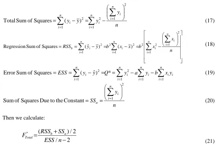
2.2. Testing for the Significance of the Entire Linear Equation
This test consists of testing the hypothesis:
1. H0: α = β = 0 vs H0: α and β are not both equal to 0, or
2. H0: The Entire Regression equation is not significant vs H1: The Entire Regression equation is
significant
For a given bivariate data set and a given α value, we need to first calculate:
n y y y y n i i n i i n i i 2 1 1 2 1 2 ) ( Squares of Sum Total − = − =
∑
∑
∑
= = = (17) − = − = − = =∑
∑
∑
∑
= = = = n x x b x x b y y RSS n i i n i i n i i n i i b 2 1 1 2 2 1 2 2 1 2 ) ( ) ˆ ( Squares of SumRegression (18)
∑
∑
∑
∑
= = = = − − = = − = = n i i i n i i n i i n ii y Q y a y b x y
y ESS 1 1 1 2 1 2 * ) ˆ ( Squares of Sum
Error (19)
n y SS n i i a 2 1 Constant the to Due Squares of Sum = =
∑
= (20)Then we calculate:
F
Total*
=
(RSS
b+
SS
a) / 2
ESS / n
−
2
(21)and compare F*
Total to F2n-2(α), which is a tabulated value, for a specified α value. If F*Total > F2n-2(α),
we reject H0 and conclude that the entire regression equation (i.e. ŷ=a+bx) or that both the constant term a,
and the factor x (and term bx) are significant to the calculation of the y value, simultaneously.
Note 1:
When TSS, RSSb, and ESS are known, we can also define the coefficient of determination R²,
where:
R
2=
RSS
bTSS
=
1
−
ESS
TSS
(22)where 0 ≤ R2≤ 1, which tells us how well the regression equation ŷ = a + bx fits the given bivariate
data. A value of R close to 1 implies a good fit. Note 2:
. = /.. 0 ,1/2 / 331 1 2, = √5 (23)
2.3. A Bivariate Example
A sample of 5 adult men for whom heights and weights are measured gives the following results (Table 1):
Table 1. Given bivariate data set (n =5)
x = H y = W x2=H2 y2=W2 xy = HW
Expert Journal of Business and Management, 3(2), pp.205-228
For this Bivariate Data set we have: n = 5
∑
= 5 1 330 = 68 + 67 + 66 + 65 + 64 = i i x 21,790 = 68² + 67² + 66² + 65² + 64² = 5 1 2∑
= i i x 760 = 170 + 165 + 150 + 145 + 130 = 5 1∑
= i i y=130²+145²+150²+165²+170²=116,550
5 1 2
∑
= i i y=(64 x 130)+(65 x 145)+(66 x 150)+(67 x 165)+(68 x 170)=50,260
5 1 i i iy x
∑
=To obtain the linear equation ŷ = a + bx, we substitute the values of n,
x
ii=1 5
∑
,x
i2i=1 5
∑
,x
ii=1 5
∑
y
ito equations (8) and (9) and obtain:
6330 + 21,790 = 50,2605 + 330 = 760
When these equations are solved simultaneously we obtain: a = -508 and b = 10, and the regression equation is
ŷ = a + bx = −508 + 10x.
Then, using the values of a = -508, b=10, and
y
ii=1 5
∑
,y
i2i=1 5
∑
andx
ii=1 5
∑
y
iwe obtain from equation (12):
ˆ
σ
=
116, 550
−
(
−
508)(760)
−
(10)(50, 260)
5
−
2
1/2=
30
3
1/2=
10
=
3.16228
and from equations (10) and (11):
66.015 = 4358 = 10 790 , 21 2 10 790 , 21 2 5 ) 330 ( 790 , 21 790 , 21 5 10 ) ( 2 / 1 2 / 1 2 / 1 2 = = − = x a
σ
σ
(b)
=
10
21, 790
−
(330)
2
5
1/2=
10
10
[ ]
1/2=
10
10
=
1
Since n=5<30, a and b are distributed as
t
n−2=
t
3variables and when α = 0.05, t3(α/2) = t3(0.025) == ±3.1824.
Then the hypotheses H0: β = 0 vs. H1: β≠ 0, and H0: α = 0 vs. H0: α≠ 0 are both rejected because: ,∗
= ( =66,015 = −7.695 < −3.1824−508
and
,∗
Therefore, the final equation is
ŷ = a + bx = −508 + 10x.
To test for the significance of the entire equation, and to calculate the coefficient of determination, we first evaluate, TSS, RSSb, ESS, SSa using equations (17) – (20) and obtain:
1030
5
)
760
(
-116,550
=
TSS
2
=
1000
)
10
(
10
5
)
330
(
790
,
21
10
22
2
=
=
−
=
b
RSS
30 10(50,260)
-) (-508)(760
-116,550 =
ESS =
115,520
=
5
)
760
(
=
2
a
SS
From equation (22), we obtain R2 = 1000/1030 ≈ 0.971, which tells us that 97% of the variation in
the values of Y can be explained (or are accounted for) by the variable X included in the regression equation and only 3% is due to other factors. Since R2 is close to 1, the fit of the equation to the data is very good.
Note:
The correlation coefficient r, which measures the strength of the linear relationship between Y and X is related to the coefficient of determination by:
0.985
97
.
0
=
r
R
2=
=
for this example. Clearly X and Y are very strongly linearly related. Using equation (21) we obtain:
5,826 = 10
260 , 58 3
/ 30
2 / ) 520 , 115 1000 ( 2 /
2 / ) (
* = + =
− + =
n ESS
SS RSS
F b a
Total
when F*
Total is compared to
F
n2−2(
α
)
=
F
32(
α
)
=
10.13 if
α
=
0.05
34.12 if
α
=
0.01
H0 (The entire regression equation is not significant) is rejected, and we conclude that the entire
regression equation is significant.
3. MINITAB Solution to the Linear Regression Problem
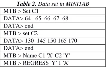
We enter the given data and issue the regression command as shown in Table 2.
Table 2. Data set in MINITAB MTB > Set C1
DATA> 64 65 66 67 68 DATA> end
MTB > set C2
DATA> 130 145 150 165 170 DATA> end
MTB > Name C1 'X' C2 'Y' MTB > REGRESS 'Y' 1 'X'
Expert Journal of Business and Management, 3(2), pp.205-228
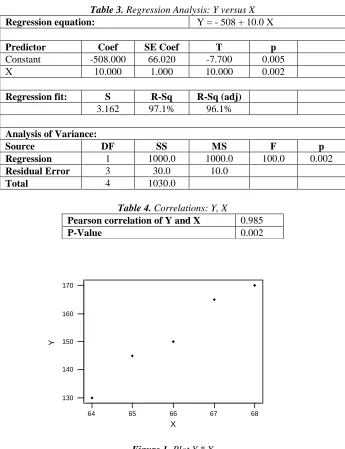
Table 3. Regression Analysis: Y versus X
Regression equation: Y = - 508 + 10.0 X
Predictor Coef SE Coef T p
Constant -508.000 66.020 -7.700 0.005
X 10.000 1.000 10.000 0.002
Regression fit: S R-Sq R-Sq (adj)
3.162 97.1% 96.1%
Analysis of Variance:
Source DF SS MS F p
Regression 1 1000.0 1000.0 100.0 0.002
Residual Error 3 30.0 10.0
Total 4 1030.0
Table 4. Correlations: Y, X
Pearson correlation of Y and X 0.985
P-Value 0.002
64 65 66 67 68
130 140 150 160 170
X
Y
Figure 1. Plot Y * X
When we compare the MINITAB and hand solutions, they are identical. We obtain the same equation ŷ = -508 + 10x, the same standard deviations for a and b (under SE Coefficient) and the same t values, the same R2, the same s = σ and σ2 = 10. Notice also that an Analysis of Variance table provides the
values for RSSb, ESS, and TSS. The only value missing is SSa, which can be easily calculated from
SS
a=
y
i i=1n
∑
2
n
.The MINITAB solution also gives a p-value for each coefficient. The p-value is called the “Observed Level of Significance” and represents the probability of obtaining a value more extreme than the value of the test statistic. For example the p-value for the predictor X is calculated as p = 0.002, and it is given by:
002
.
0
)
(
=
10)
=
*
t
>
P(t
=
value
-p
10
=
∫
∞f
t
dt
(24)If p < α, reject H0
Since p = 0.002 < α = 0.05, H0: β = 0 will be rejected.
4. Introduction and Model Estimation for Some Non-Linear Models of Interest
Sometimes two variables are related but their relationship is not linear and trying to fit a linear equation to a data set that is inherently non-linear will result in a bad-fit. But, because non-linear regression is, in general, much more difficult than linear regression, we explore in this part of the paper estimation methods that will allow us to fit non-linear equations to a data set by using the results of linear regression which is much easier to understand and analyze.
This becomes possible by first performing logarithmic transformations of the non-linear equations, which change the non-linear into linear equations, and then using the normal equations of the linear model to generate the normal equations of the “linearized” non-linear equations, from which the values of the unknown model parameters can be obtained. In this paper we show how the exponential model, ŷ = kecx, and
the power model, ŷ = axb (for b≠1) can be easily estimated by using logarithmic transformations to first
derive the linearized version of the above non-linear equations, namely:
cx
k
y
ˆ
=
ln
+
ln
and
x
b
a
y
ˆ
ln
ln
ln
=
+
,and then comparing these to the original linear equation, ŷ = a + bx, and its normal equations (see equations (8) and (9)).
Also discussed is the quadratic model, ŷ = a + bx + cx2 which, even though is a non-linear model,
can be discussed directly using the linear methodology. But now we have to solve simultaneously a system of 3 equations in 3 unknowns, because the normal equations for the quadratic model become:
∑
∑
∑
= =
=
=
+
+
ni
n
i i i
n
i
i
c
x
y
x
b
na
1 1 2 1
∑
∑
∑
∑
= = =
=
=
+
+
ni
n
i i i n
i i i
n
i
i
b
x
c
x
x
y
x
a
1 1 1
3 2
1
(25)
∑
∑
∑
∑
= = =
=
=
+
+
ni
n
i i i n
i i i
n
i
i
b
x
c
x
x
y
x
a
1 1
2 1
4 3
1 2
A procedure is also discussed which allows us to fit these four models (i.e. linear, exponential, power, quadratic), and possibly others, to the same data set, and then select the equation which fits the data set “best”. These four models are used extensively in forecasting and, because of this, it is important to understand how these models are constructed and how MINITAB can be used to estimate such models efficiently.
4.1. The Linear Model and its Normal Equations
The linear model and the normal equations associated with it as explained above, are given by:
Linear Model
= + (1)
Normal Equations
∑
∑
= =
=
+
ni i n
i
i
y
x
b
na
1 1
(8)
∑
∑
∑
= =
=
=
+
ni i i n
i i n
i
i
b
x
x
y
x
a
1 1
2 1
Expert Journal of Business and Management, 3(2), pp.205-228
4.2. The Exponential Model
The exponential model is defined by the equation:
cx
ke
y
ˆ
=
(26)Our objective is to use the given data to find the best possible values for k and c, just as our objective in equation (1) was to use the data to find the best (in the least-square sense) values for a and b.
Taking natural logarithms (i.e. logarithms to the base e) of both sides of equation (26) we obtain
)
ˆ
ln(
y
=
ke
cxor
)
ln(
ˆ
ln
y
=
ke
cx (27)4.2.1. Logarithmic Laws
To simplify equation (27), we have to use some of the following laws of logarithms:
i) log (A·B) = log A + log B (28)
ii) log (A/B) = log A – log B (29)
iii) log (An) = n log A (30)
Then, using equation (28) we can re-write equation (27) as:
cx
e
k
y
ln
ln
ln
=
+
(31)and, by applying equation (30) to the second term of the right hand side of equation (31), equation (31) can be written finally as:
) (ln ln
lny= k +cx e
or
cx k
y=ln +
ln (because ln e = loge e = 1) (32)
Even though equation (26) is non-linear, as can be verified by plotting y against x, equation (32) is linear (i.e. the logarithmic transformation changed equation (26) from non-linear to linear) as can be verified by plotting: ln y against x.
But, if equation (32) is linear, it should be similar to equation (1), and must have a set of normal equations similar to the normal equations of the linear model (see equations (8) and (9)).
Question: How are these normal equations going to be derived?
Answer: We will compare the “transformed linear model”, i.e. equation (32), to the actual linear
model (equation (1)), note the differences between these two models, and then make the appropriate changes to the normal equations of the linear model to obtain the normal equations of the “transformed linear model”.
4.2.2. Comparison of the Logarithmic Transformed Exponential Model to the Linear Model
To make the comparison easier, we list below the 2 models under consideration, namely: a) Original Linear Model:
= + (1)
b) Transformed Linear Model:
cx k
y=ln +
ln (32)
Comparing equations (1) and (32), we note the following three differences between the two models: i. y in equation (1) has been replaced by ln y in equation (32)
ii. a in equation (1) has been replaced by ln k in equation (32)
4.2.3. Normal Equations of Exponential Model
When the three changes listed above are applied to the normal equations of the actual linear model (equations (8) and (9)), we will obtain the normal equations of the “transformed model”. The normal equations of the “transformed linear model” are:
∑
∑
= =
=
+
ni i n
i
i
y
x
c
k
n
1 1
ln
)
(ln
(33))
(ln
)
(ln
1 1
2 1
∑
∑
∑
= =
=
=
+
ni
i i n
i i n
i
i
c
x
x
y
x
k
(34)In equations (33) and (34) all the quantities are known numbers, derived from the given data as will be shown later, except for: ln k and c, and equations (33) and (34) must be solved simultaneously for ln k and c.
Suppose that for a given data set, the solution to equations (33) and (34) produced the values:
ln k = 0.3 and c = 1.2 (35)
If we examine the exponential model (equation (26)), we observe that the value of c = 1.2 can be substituted directly into equation (26), but we do not yet have the value of k; instead we have the value of ln
k = 0.3!
Question: If we know: ln k = 0.3, how do we find the value of k?
Answer: If ln k = 0.3, then: k = e0.3
≈
(2.718281828)0.3≈
1.349859Therefore, now that we have both the k and c values, the non-linear model, given by equation (26), has been completely estimated.
4.3.The Power Model
Another non-linear model, which can be analyzed in a similar manner, is the Power Model defined by the equation:
b
ax
y
ˆ
=
(36)which is non-linear if b ≠ 1 and, as before, we must obtain the best possible values for a and b (in the least-square sense) using the given data.
4.3.1. Logarithmic Transformation of Power Model
A logarithmic transformation of equation (36) produces the “transformed linear model”
x b a
y ln ln
ln = + (37)
When equation (37) is compared to equation (1), we note the following 3 changes: i. y in equation (1) has been replaced by ln y in equation (37)
ii. a in equation (1) has been replaced by ln a in equation (37) (38) iii. x in equation (1) has been replaced by ln x in equation (37)
When the changes listed in (38) are substituted into equations (8) and (9), we obtain the normal equations for this “transformed linear model” which are given by equations (39) and (40) below:
4.3.2. Normal Equations of Power Model
∑
∑
= =
=
+
ni i n
i
i
y
x
b
a
n
1 1
ln
ln
)
(ln
(39))
)(ln
(ln
)
(ln
ln
)
(ln
1 1
2 1
∑
∑
∑
= =
=
=
+
ni
i i n
i
i n
i
i
b
x
x
y
x
Expert Journal of Business and Management, 3(2), pp.205-228
Equations (39) and (40) must be solved simultaneously for (ln a) and b.
If ln a = 0.4, then a = e0.4≈ (2.718251828)0.4≈ 1.491825 and, since we have numerical values for
both a and b, the non-linear model defined by equation (36) has been completely estimated.
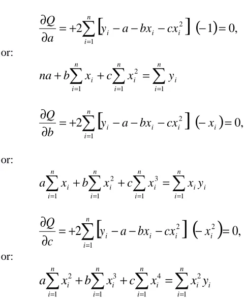
4.4. Derivation of the normal equations for the Quadratic model, y = a + bx + cx2
To derive the normal equations of the quadratic model, first form the function
[
]
∑
=−
−
−
n i i ii
a
bx
cx
y
1 2 2=
c)
b,
Q(a,
(41)
Then take the partial derivatives:
,
,
,
c
Q
b
Q
a
Q
∂
∂
∂
∂
∂
∂
and set each equal to 0, to obtain the 3 equations
needed to solve for a, b, c. We obtain:
[
]
( )
∑
==
−
−
−
−
+
=
∂
∂
n i i ii
a
bx
cx
y
a
Q
1 2,
0
1
2
or:∑
∑
∑
= = ==
+
+
n i n i n i i ii
c
x
y
x
b
na
1 1 1
2 (42)
[
]
( )
∑
==
−
−
−
−
+
=
∂
∂
n i i i ii
a
bx
cx
x
y
b
Q
1 2,
0
2
or:∑
∑
∑
∑
= = = ==
+
+
n i n i n i i i n i i ii
b
x
c
x
x
y
x
a
1 1 1 1
3 2 (43)
[
]
( )
∑
==
−
−
−
−
+
=
∂
∂
n i i i ii
a
bx
cx
x
y
c
Q
1 2 2,
0
2
or:∑
∑
∑
∑
= = = ==
+
+
n i n i n i i i n i i ii
b
x
c
x
x
y
x
a
1 1 1
2 1 4 3 2 (44)
Equations (42), (43), and (44) are identical to equation (25).
4.5. Data Utilization in Estimating the 4 Models
To generate the quantities needed to estimate the 4 models: a. The Linear Model
b. The Exponential Model c. The Power Model, d. The Quadratic Model,
the given (x, y) bivariate data must be “manipulated” as shown in Tables: 5, 6, 7, and 8, respectively.
4.5.1. Given Data to Evaluate the Linear Model
Table 5. Manipulation of Given Data to Evaluate the Linear Model x y xy x2
x1 y1 x1y1 x12
x2 y2 x2y2 x22
x3 y3 x3y3
… … … …
xn yn xnyn
2
n
x
xn2
∑
= n i ix
1∑
= n i iy
1∑
= n i i iy
x
1∑
= n i ix
1 2N1 N2 N3 N4
To evaluate y = a + bx, substitute: N1, N2, N3, N4 into equations (8) and (9) and solve for a and b
simultaneously.
4.5.2. Given Data to Evaluate the Exponential Model
Table 6. Manipulation of Given Data to Evaluate the Exponential Model
x y x2 ln y x ln y
x1 y1 2
1
x
ln y11 1
ln y
x
⋅
x2 y2 2
2
x
ln y22 2
ln y
x
⋅
x3 y3 2
3
x
ln y33 3
ln y
x
⋅
… … … … …
xn yn 2
n
x
ln ynn n
y
x ln
⋅
∑
= n i ix
1∑
= n i iy
1∑
= n i ix
1 2∑
= n i iy
1ln
∑
= n i i iy
x
1ln
N5 N6 N7 N8 N9
To evaluate
y
=
ke
cx, substitute N5, N7, N8, N9 into equations (33) and (34) and solve for ln k and csimultaneously.
4.5.3. Given Data to Evaluate the Power Model
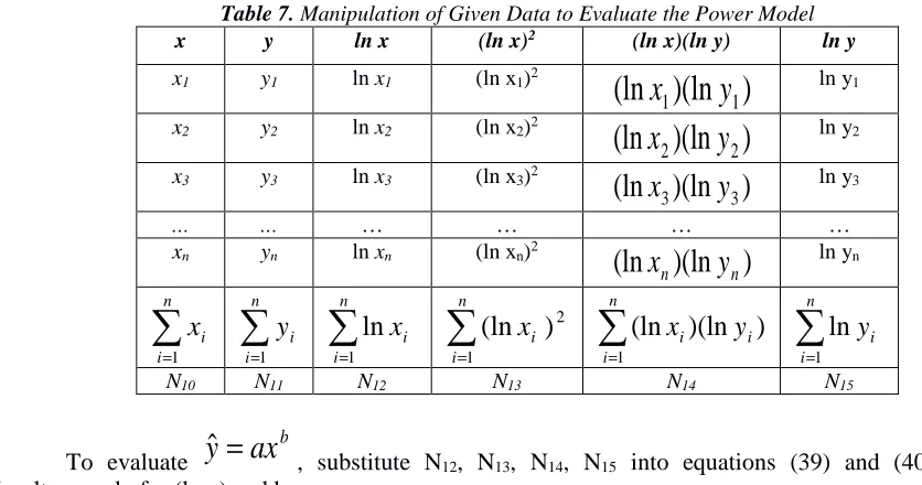
Table 7. Manipulation of Given Data to Evaluate the Power Model
x y ln x (ln x)2 (ln x)(ln y) ln y
x1 y1 ln x1 (ln x1)2
(ln
)(ln
)
1
1
y
x
ln y1x2 y2 ln x2 (ln x2)2
(ln
)(ln
)
2
2
y
x
ln y2x3 y3 ln x3 (ln x3)2
(ln
)(ln
)
3
3
y
x
ln y3… … … … … …
xn yn ln xn (ln xn)2
(ln
)(ln
)
n n
y
x
ln yn∑
= n i ix
1∑
= n i iy
1∑
= n i ix
1ln
∑
= n i ix
1 2)
(ln
∑
= n i i iy
x
1)
)(ln
(ln
∑
= n i iy
1ln
N10 N11 N12 N13 N14 N15
To evaluate
b
ax
y
ˆ
=
, substitute N12, N13, N14, N15 into equations (39) and (40) and solve
Expert Journal of Business and Management, 3(2), pp.205-228
4.5.4. Given Data to Evaluate the Quadratic Model
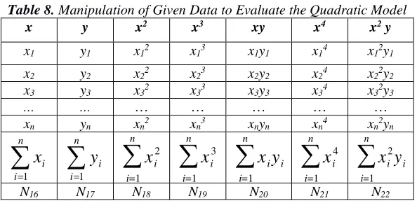
Table 8. Manipulation of Given Data to Evaluate the Quadratic Model
x y x2 x3 xy x4 x2 y
x1 y1 x12 x13 x1y1 x14 x12y1 x2 y2 x22 x23 x2y2 x24 x22y2 x3 y3 x32 x33 x3y3 x34 x32y3
… … … … … … …
xn yn xn2 xn3 xnyn xn4 xn2yn
∑
=
n
i i
x
1
∑
=
n
i i
y
1
x
i2
i=1
n
∑
x
i3
i=1
n
∑
x
ii=1
n
∑
y
ix
i4
i=1
n
∑
x
i2
i=1
n
∑
y
iN16 N17 N18 N19 N20 N21 N22
To evaluate = + + , substitute N16, N17, N18, N19, N20, N21, N22 into equations (42),
(43), and (44), and solve simultaneously for a, b, and c.
5. Selecting the Best-Fitting Model
5.1. The Four Models Considered
Given a data set (xi, yi), we have shown how to fit to such a data set four different models, namely:
a. Linear:
y
ˆ
i=
a
+
bx
i (45)b. Exponential:
i
cx i
ke
y
ˆ
=
(46)c. Power:
b i i
ax
y
ˆ
=
(47)d. Quadratic:
2 ˆi a bxi cxi
y = + + (48)
We might decide to fit all four models to the same data set if, after examining the scatter diagram of the given data set, we are unable to decide which of the “4 models appears to fit the data BEST.”
But, after we fit the 4 models, how can we tell which model fits the data best?
To answer this question, we calculate the “variance of the residual values” for each of the models, and then “select as the best model” the one with the smallest variance of the residual values.
5.2. Calculating the Residual Values of Each Model and Their Variance
Use each xi value, of the given data set (xi, yi), to calculate the
yˆ
i value, from the appropriatemodel, and then for each i, form the residual:
)
ˆ
(
=
ns
observatio
of
Residual
y
i−y
i , (49)for each i.
Then the variance of the residual values is defined by:
2 1
)
ˆ
(
1
=
(Residual)
V
∑
=
−
ni
i
i
y
y
DOF
, (50)where DOF = Degrees of Freedom.
Note: The DOF are DOF = n – 2 for the first three models (Linear, Exponential, Power) due to the
Using equation (50) to calculate the variance of the residuals for each of the 4 models, we obtain:
2
1
Linear
(
)
2
1
=
(Residual)
V
∑
=−
−
−
n i ii
a
bx
y
n
(51)
[
(
1 1) (
2 2 2)
2 ...(
)
2]
2 1
n n a bx
y bx a y bx a y
n− − − + − − + + − −
= (52)
2
1
l
Exponentia
(
)
2
1
=
(Residual)
V
∑
=−
−
n i cx i ike
y
n
(53)
[
2 2]
2 2
1 ) ( ) ( )
( 2
1 1 2 cxn
n cx cx ke y ke y ke y
n− − + − + + −
= L (54)
2
1
Power
(
)
2
1
=
(Residual)
V
∑
=−
−
n i b i iax
y
n
(55)
[
2 2]
2 2 2 1
1 ) ( ) ( )
( 2 1 b n n b b ax y ax y ax y
n− − + − + + −
= L (56)
∑
=−
−
−
−
n i i ii
a
bx
cx
y
n
12 2
Quadratic
(
)
3
1
=
(Residual)
V
(57)[
2 2 2 2]
2 2 2 2 2 1 1
1 ) ( ) ... ( )
( 3 1
n n n a bx cx
y cx bx a y cx bx a y
n− − − − + − − − + + − − −
= (58)
After the calculation of the 4 variances from equations: (52), (54), (56), and (58), the model with the “smallest” variance is the model which fits the given data set “best”.
We will now illustrate, through an example, how the 4 models we discussed above can be fitted to a given bivariate data set, and then how the “best” model from among them is selected.
5.3. A Considered Example
A sample of 5 adult men for whom heights and weights are measured gives the following results (Table 9).
Table 9. Sample of 5 adult men # X = Height Y = Weight
1 64 130
2 65 145
3 66 150
4 67 165
5 68 170
Problem: Fit the linear, exponential, power, and quadratic models to this bivariate data set and then select as the “best” the model with the smallest variance of the residual values.
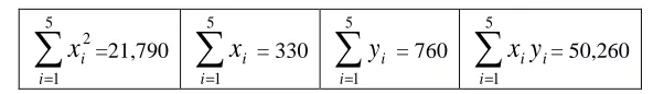
5.3.1. Fitting the Linear Model ˆy =a + bx
To fit the linear model, we must extend the given bivariate data so that we can also calculate
∑
= n i ix
1 2and i
n i i
y
x
∑
=1, as shown below, in Table 10:
Table 10. Calculations for bivariate data of 5 adults for the linear model
x2 x y Xy
4096 64 130 8320
4225 65 145 9425
4356 66 150 9900
4489 67 165 11055
Expert Journal of Business and Management, 3(2), pp.205-228
∑
=
5
1 2
i i
x
=21,790∑
=
5
1
i i
x
= 330∑
=
5
1
i i
y
= 760 ii i
y
x
∑
=
5
1
= 50,260
We then substitute the generated data into the normal equations for the linear model, namely equations (8) and (9):
∑
∑
= =
=
+
ni i n
i
i
y
x
b
na
1 1
∑
∑
∑
= =
=
=
+
ni i i n
i i n
i
i
b
x
x
y
x
a
1 1
2
1
,
and obtain the equations:
6330 + 21,790 = 50,2605 + 330 = 760
When these equations are solved simultaneously for a and b we obtain:
G = −508, 2H= 10
Therefore, the linear model is:
ŷ = a + bx = −508 + 10x
The variance of the residual values for the linear model is calculated as shown below, in Table 11:
Table 11. Variance of the residual values for the linear model
Given X Given Y Calculated Y Residual (Residual)2
x y yˆ= -508 + 10x y - yˆ (y - yˆ)2
64 130 -508 + 10 (64) = 132 -2 (-2)2 = 4 65 145 -508 + 10 (65) = 142 +3 (+3)2 = 9 66 150 -508 + 10 (66) = 152 -2 (-2)2 = 4 67 165 -508 + 10 (67) = 162 +3 (+3)2 = 9 68 170 -508 + 10 (68) = 172 -2 (-2)2 = 4
30
)
ˆ
(
25
1
=
−
∑
=
i
i
i
y
y
Therefore, the variance of the residual values, for the linear model is:
10
3
30
)
30
(
2
5
1
)
ˆ
(
2
1
=
)
V(Residual
21
Linear
=
=
−
=
−
−
∑
=n
i
i
i
y
y
n
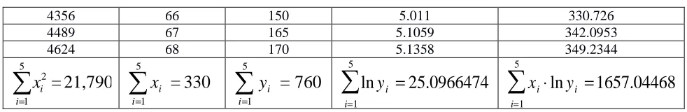
5.3.2. Fitting the Exponential Model ŷ = kecx
To fit the exponential model we need to extend the given bivariate data so that we can calculate, in
addition to
=
330
5
1
∑
=
i i
x
and=
21,790
5
1 2
∑
=
i i
x
,∑
=
5
1
ln
i i
y
and(x
iln y
ii=1 5
∑
)
as shown below, in Table 12:Table 12. Calculations for bivariate data of 5 adults for the exponential model
x2 x y ln y x⋅ln y
4096 64 130 4.8675 311.5200
4356 66 150 5.011 330.726
4489 67 165 5.1059 342.0953
4624 68 170 5.1358 349.2344
21,790
=
5 1 2∑
= i ix
=
330
5 1
∑
= i ix
=
760
5 1
∑
= i iy
ln y
ii=1 5
∑
=
25.0966474
x
i⋅
ln y
ii=1 5
∑
=
1657.04468
We then substitute the generated data into the normal equations for the exponential model (i.e. equations (33) and (34)):
∑
∑
= ==
+
n i i n i iy
x
c
k
n
1 1ln
)
(ln
)
(ln
)
(ln
1 1 2 1∑
∑
∑
= = ==
+
n i i i n i i n ii
c
x
x
y
x
k
,and obtain the equations:
630 ln + 21,790 = 1657.04475 ln + 330 = 25.0967
When these equations are solved simultaneously for ln k and c, we obtain: c = 0.06658 and lnk = 0.6251, or: k = e0.6251 = 1.868432
Therefore, the exponential model is: x cx
ke
y
ˆ
=
=
1.868432
e
0.06658or
ln y = ln k + cx = 0.6251 + 0.06658x
Then, the variance of the residual values, for the exponential model, is calculated as shown below, in Table 13:
Table 13. Variance of the residual values for the exponential model x y yˆ= kecx = 1.868432 e0.06658x y - yˆ (y - yˆ)2
64 130 1.868432 e0.06658(64) = 132.4515 -2.4515 6.0099 65 145 1.868432 e0.06658(65) = 141.5703 3.4297 11.7628 66 150 1.868432 e0.06658(66) = 151.3169 -1.3169 1.7324 67 165 1.868432 e0.06658(67) = 161.7346 3.2654 10.6630 68 170 1.868432 e0.06658(68) = 172.8694 -2.8694 8.2336
4035
.
38
)
ˆ
(
2 5 1=
−
∑
= i i iy
y
Therefore, the variance of the residual values, for the exponential model is:
2 1 2 1 l
Exponentia
(
)
2
1
)
ˆ
(
2
1
=
)
V(Residual
∑
∑
= =
−
−
=
−
−
n i cx i n i i i ike
y
n
y
y
n
[
]
2Expert Journal of Business and Management, 3(2), pp.205-228
5.3.3. Fitting the Power Model, ŷ = axb
To fit the power model we need to extend the given bivariate data set to generate the quantities:
∑
=
n
i i
x
1
ln
, 21
)
(ln
∑
=
n
i
i
x
,∑
=
n
i i
y
1
ln
and(ln
)(ln
)
1
∑
=
n
i
i
i
y
x
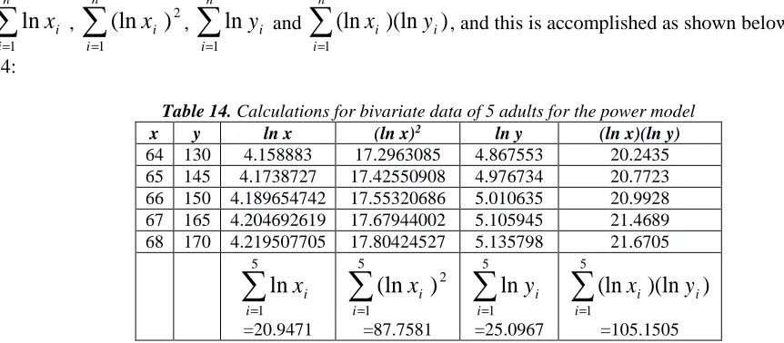
, and this is accomplished as shown below, in Table14:
Table 14. Calculations for bivariate data of 5 adults for the power model
x y ln x (ln x)2 ln y (ln x)(ln y)
64 130 4.158883 17.2963085 4.867553 20.2435 65 145 4.1738727 17.42550908 4.976734 20.7723 66 150 4.189654742 17.55320686 5.010635 20.9928 67 165 4.204692619 17.67944002 5.105945 21.4689 68 170 4.219507705 17.80424527 5.135798 21.6705
∑
=
5
1
ln
i i
x
=20.9471
2 5
1
)
(ln
∑
=
i
i
x
=87.7581
∑
=
5
1
ln
i i
y
=25.0967
)
)(ln
(ln
5
1
∑
=
i
i
i
y
x
=105.1505
We then substitute the generated data into the normal equations of the power model, namely equations (39) and (40):
∑
∑
= =
=
+
ni i n
i
i
y
x
b
a
n
1 1
ln
ln
)
(ln
)
)(ln
(ln
)
(ln
ln
)
(ln
1 1
2
1
∑
∑
∑
= =
=
=
+
ni
i i n
i i n
i
i
b
x
x
y
x
a
and obtain the equations:
G20.9471 ln + 87.7581 = 105.15055 ln + 20.9471 = 25.0967
When these equations are solved simultaneously for b and ln a we obtain:
G = 4.3766, 2Hln = −13.316
Therefore, the “linearized” power model becomes:
ln ŷ = ln + ln = −13.316 + 4.3766
Then the variance of the residual values for the power model is obtained as shown below:
Table 15. Variance of the residual values for the power model
x y ln x ln yˆ = ln a + b ln x
= -13.316 + 4.3766x yˆ y - yˆ (y - yˆ)
2
64 130 4.158883 ln yˆ1 = 4.885768 132.3920 -2.3920 5.721664
65 145 4.173873 ln yˆ2 = 4.95623 141.6874 3.3126 10.973319
66 150 4.189655 ln yˆ3 = 5.020443 151.4784 -1.47843 2.185667
67 165 4.204693 ln yˆ4 = 5.086258 161.7833 3.2167 10.347159
68 170 4.219508 ln yˆ5 = 5.151097 172.6208 -2.6208 6.868592
i=1 5
∑
(yi -yˆ
i)2Therefore, the variance of the residuals values for the power model is:
12.0321 =
3 0964 . 36 ) (
2 1 = )
V(Residual 2
1
Power − =
−
∑
= ni
b i i ax y
n
5.3.4. Fitting the Quadratic Model,ŷ = a + bx +cx2
To fit the quadratic model, we need to use the given bivariate data set and extend it to generate the quantities:
X
i=
330;
X
i2i=1
n
∑
=
21,790
i=1
n
∑
;
X
i3i=1
n
∑
=
1, 439,460;
X
i4=
95,135,074;
i=1n
∑
Y
ii=1
n
∑
=
760;
X
iY
i=
50,260;
i=1n
∑
X
i2Y
i=
3,325,270
i=1
n
∑
We then substitute the generated data into the normal equations of the quadratic model (see equation (25)), and obtain:
K 330a + 21,790b + 1,439,460c = 50,2605a + 330b + 21,790c = 760 21,790a + 1,439,460b + 95,135,074c = 3,325,270
Solving these 3 equations simultaneously, we obtain a = -25,236/7, b = 730/7, c = -5/7. Therefore, the quadratic function ŷ = f(x) is given by:
ŷ = a + bx + cx2 =17 [−23,326 + 730 − 5 ]
The variance of the residual values for the quadratic model is calculated as shown below, in Table 16:
Table 16. Variance of the residual values for the quadratic model
x y yˆ =
1
7
−
25,326
+
730 x
−
5x
2
[
]
yi - yˆi (yi - yˆi)264 130 yˆ1 = 130.5714286 -0.5714286 0.326530644
65 145 yˆ2 = 142.7142857 2.2857143 5.224489861
66 150 yˆ3 = 153.4285714 -3.4285714 11.75510184
67 165 yˆ4 = 162.7142857 2.2857143 5.224489861
68 170 yˆ5 = 170.5714286 -0.5714286 0.326530644
i=1 5
∑
(yi - yˆi)2= 22.85714286
Therefore, the variance of the residual values for the quadratic model is:
4286 . 11 42857143 .
11 2
85714286 .
22 ) ˆ -(y 3 1 )
V(Residual
5
1
2
Quadratic i i = = ≈
−
=
∑
=
i
y n
5.3.5. Summary of Results and Selection of the “Best” Model
Expert Journal of Business and Management, 3(2), pp.205-228
a) The linear model is:
10x 508 -bx + a
ˆ = = +
y
with V(Residual)Linear = 10
b) The exponential model is:
x cx
ke
y
ˆ
=
=
1.868432
e
0.06658with V(Residual)Exponential = 12.8017
c) The power model is:
ln x 4.3766 + 13.316 -= ln x b + a ln ˆ ln y =
with V(Residual)Power = 12.0321
d) The quadratic model is
[
2]
2
5 730 326 , 25 7 1 = cx + bx + a
ˆ x x
y= − + −
with V(Residual) Quadratic = 11.4286
Since the linear model has the smallest variance of the residual values of the 4 models fitted to the same bivariate data set, the linear model is the “best” model (but the other 3 values are very close). The linear model, therefore, will be selected as the “best” model and used for forecasting purposes.
6. MINITAB Solutions
To obtain the MINITAB solutions of the four models we discussed in this paper we do the following:
6.1. Finding the MINITAB Solution for the Linear Model
The data set used to find the MINITAB solution for the linear model is presented in Table 17.
Table 17. Data set in MINITAB for the linear model MTB > Set C1
DATA> 64 65 66 67 68 DATA> end
MTB > set C2
DATA> 130 145 150 165 170 DATA> end
MTB > Name C1 'X' C2 'Y' MTB > REGRESS 'Y' 1 'X'
The results of the regression analysis for the linear model is presented in Table 18.
Table 18. Regression analysis: Y versus X for the linear model
Regression equation: Y = - 508 + 10.0 X
Predictor Coef SE Coef T p
Constant -508.000 66.020 -7.700 0.005
X 10.000 1.000 10.000 0.002
Regression fit: S R-Sq R-Sq (adj)
Analysis of Variance:
Source DF SS MS F p
Regression 1 1000.0 1000.0 100.0 0.002
Residual Error 3 30.0 10.0
Total 4 1030.0
6.2. Finding the MINITAB Solution for the Exponential Model
The data set used to find the MINITAB solution for the exponential model is presented in Table 19.
Table 19. Data set in MINITAB for the exponential model MTB > Set C1
DATA> 64 65 66 67 68 DATA> end
MTB > set C2
DATA> 130 145 150 165 170 DATA> end
MTB > Name C1 'X' C2 'Y' MTB > REGRESS 'Y' 1 'X'
The results of the regression analysis for the exponential model is presented in Table 20.
Table 20. Regression analysis: Y versus X for the exponential model
Regression equation: Y = 0.625 + 0.0666 X
Predictor Coef SE Coef T p
Constant 0.6251 0.4925 1.27 0.294
X 0.066580 0.007460 8.92 0.003
Regression fit: S R-Sq R-Sq (adj)
0.0235917 96.4% 95.2%
Analysis of Variance:
Source DF SS MS F p
Regression 1 0.044329 0.044329 79.65 0.003
Residual Error 3 0.001670 0.000557
Total 4 0.045999
6.3. Finding the MINITAB Solution for the Power Model
The data set used to find the MINITAB solution for the power model is presented in Table 21.
Table 21. Data set in MINITAB for the power model MTB > Set C1
DATA> 4.158883; 4.1738727; 4.189654742; 4.204692619; 4.2195077 DATA> end
MTB > set C2
DATA> 4.867553; 4.976734; 5.010635; 5.105945; 5.135798 DATA> end
MTB > Name C1 'X' C2 'Y' MTB > REGRESS 'Y' 1 'X'
Expert Journal of Business and Management, 3(2), pp.205-228
Table 22. Regression analysis: Y versus X for the power model
Regression equation: Y = - 13.3 + 4.38X
Predictor Coef SE Coef T p
Constant -13.316 2.069 -6.44 0.008
X 4.3766 0.4939 8.86 0.003
Regression fit: S R-Sq R-Sq (adj)
0.0237507 96.3% 95.1%
Analysis of Variance:
Source DF SS MS F p
Regression 1 0.044301 0.044301 78.53 0.003
Residual Error 3 0.001692 0.000564
Total 4 0.045993
6.4. Finding the MINITAB Solution for the Wuadratic Model
The data set used to find the MINITAB solution for the quadratic model is presented in Table 23.
Table 23. Data set in MINITAB for the quadratic model MTB > Set C1
DATA> 64 65 66 67 68 DATA> end
MTB > set C2
DATA> 4096 4225 4356 4489 4624 DATA> end
MTB > SET C3
DATA> 130 145 150 165 170 DATA> END
MTB > NAME C1 'X1' C2 'X2' C3 'Y' MTB > REGRESS 'Y' 2 'X1' 'X2'
The results of the regression analysis for the quadratic model is presented in Table 24.
Table 24. Regression analysis: Y versus X1, X2 for the quadratic model
Regression equation: Y = - 3618 + 104 X1 - 0.714 X2
Predictor Coef SE Coef T p
Constant -3618 3935 -0.92 0.455
X1 104.3 119.3 0.87 0.474
X2 -0.7143 0.9035 -0.79 0.512
Regression fit: S R-Sq R-Sq (adj)
3.38062 97.8% 95.6%
Analysis of Variance:
Source DF SS MS F p
Regression 2 1007.14 503.57 44.06 0.022
Residual Error 2 22.86 11.43
Total 4 1030.00
Source DF Seg SS
X1 1 1000.00
7. Conclusions
Reviewing our previous discussion we come to the following conclusions:
The Linear Regression problem is relatively easy to solve and can be handled using algebraic methods.
The problem can also be solved easily using available statistical software, like MINITAB.
Even though the solution to Regression problems can be obtained easily using MINITAB (or other statistical software) it is important to know what the hand methodology is and how it solves these problems before you can properly interpret and understand MINITAB’s output.
In general, non-linear regression is much more difficult to perform than linear regression.
There are, however, some simple non-linear models that can be evaluated relatively easily by utilizing the results of linear regression.
The non-linear models analyzed in this paper are: Exponential Model, Power Model, Quadratic Model.
A procedure is also discussed which allows us to fit to the same bivariate data set many models (such as: linear, exponential, power, quadratic) and select as the “best fitting” model the model with the “smallest variance of the residuals”.
In a numerical example, in which all 4 of these models were fitted to the same bivariate data set, we found that the Linear model was the “best fit”, with the Quadratic model “second best”. The Power and Exponential models are “third best” and “fourth best” respectively, but are very close to each other.
The evaluation of these models is facilitated considerably by using the statistical software package MINITAB which, in addition to estimating the unknown parameters of the corresponding models, also generates additional information (such as the p-value, standard deviations of the parameter estimators, and R2).
This additional information allows us to perform hypothesis testing and construct confidence intervals on the parameters, and also to get a measure of the “goodness” of the equation, by using the value of R2. A value of R2 close to 1 is an indication of a good fit.
The MINITAB solution for the linear model shows that both a and b (of ŷ = a + bx = -508 + 10x) are significant because the corresponding p-values are smaller than α = 0.05, while the value of R2 = 97.1%,
indicating that the regression equation explains 97.1% of the variation in the y-values and only 2.9% is due to other factors.
The MINITAB solution for the quadratic model shows that a, b, and c (of ŷ = a + bx + cx2 = -3,618
+ 104.3x + 0.7143x2) are individually not significant (because of the corresponding high p-values, but b and
c jointly are significant because of the corresponding p-value of p = 0.022 < α = 0.05. The value of R2 is: R2
= 97.8%.
The MINITAB solution for the power model shows that both a and b (of ŷ = axb or ln y = ln a + b ln
x = -13.3 + 4.3766 ln x) are significant because the corresponding p-values are smaller than α = 0.05, while the value of R2 = 96.3%.
The MINITAB solution for the exponential model shows that the k (in ŷ = kecx =1.868432e0.06658x or
ln ŷ = ln k + cx = 0.6251 + 0.06658x) is not significant because of the corresponding high p-value, while the c is significant because of the corresponding p-value being smaller than α = 0.05. The value of R2 = 96.4%.
References
Adamowski, J., H., Fung Chan, S.O., Prasher, B., Ozga-Zielinski, and Sliusarieva. A., 2012. Comparison of multiple linear and nonlinear regression, autoregressive integrated moving average, artificial neural network, and wavelet artificial neural network methods for urban water demand forecasting. Water
Resources, 48, W01528, Montreal: Canada
Berenson, M.L., Levine, D.M. and Krehbiel, T.C., 2004. Basic Business Statistics (9th Edition). Upper Saddle River, N.J.: Prentice-Hall
Bhatia, N., 2009. Linear Regression: An Ap