RESEARCHARTICLE
A hidden Markov model for
matching spatial networks
Benoît Costes and Julien Perret
University Paris-Est, IGN/LaSTIG, ENSG, France
Received: January 17, 2019; returned: March 1, 2019; revised: April 9, 2019; accepted: May 16, 2019.
Abstract: Datasets of the same geographic space at different scales and temporalities are increasingly abundant, paving the way for new scientific research. These datasets require data integration, which implies linking homologous entities in a process called data match-ing that remains a challengmatch-ing task, despite a quite substantial literature, because of data imperfections and heterogeneities. In this paper, we present an approach for matching spa-tial networks based on a hidden Markov model (HMM) that takes full benefit of the under-lying topology of networks. The approach is assessed using four heterogeneous datasets (streets, roads, railway, and hydrographic networks), showing that the HMM algorithm is robust in regards to data heterogeneities and imperfections (geometric discrepancies and differences in level of details) and adaptable to match any type of spatial networks. It also has the advantage of requiring no mandatory parameters, as proven by a sensitivity ex-ploration, except a distance threshold that filters potential matching candidates in order to speed-up the process. Finally, a comparison with a commonly cited approach highlights good matching accuracy and completeness.
Keywords: spatial networks, data matching, data integration, topology, hidden Markov model, HMM
1
Introduction
whether social, administrative, or topographical. Whether based on data conflation [12, 28, 50] or on multiple representation databases [11, 43], it requires linking homologous entities from the different datasets, which is a challenging task because of data imperfections and inhomogeneities.
Linear objects representing spatial networks such as street, railway, electrical, or hydro-graphic networks are frequently encountered among the geohydro-graphical entities usually used in GIS, and are commonly the subject of many studies in geography, urbanism, sociology, or history. This article is concerned with the issue of matching linear features from spatial networks.
An extensive literature deals with matching network datasets. To find multiple match-ing links in networks of similar spatial granularity, Walter and Fritsch [46] proposed a ge-ometric approach based on statistical filtering and information theory to combine criteria. The candidate pair with the highest score is kept, and matching links are automatically assessed. To match datasets with different levels of details, Zhang et al. [51] proposed a purely geometric approach based on a growing buffer whose size is iteratively and auto-matically determined. Using a pre-matching of nodes and edges of the networks leading up to the final matching, Lüscher et al. [29], and then Mustière and Devogele [30] proposed to use adjacency relationships and calculated closest path. The former method also uses semantic information and user interventions may be needed, whereas the latter is fully automatic. Samal et al. [36] presented one of the first methods to match multiple datasets with different levels of detail at once, using multiple criteria and graph theory tools, such as maximum clique problem, as a decision process.
Multi-criteria methods have also been introduced. In order to combine multiple mea-sures, Olteanu and Mustière [32] used evidence theory [38] that models lack of knowledge, data imperfections, and ignorance. The theory of belief functions was also used by Du-menieu [13] to discover filiation relationships in several geohistorical datasets, using simu-lated annealing, whereas Tong et al. [41] chose a probabilistic approach to compute a total matching score. Optimization methods were also considered by Li and Goodchild [26, 27]. Mainly geometrical, their approach treats data matching as an assignment problem. They use combinatorial optimization to simultaneously match pairs of objects. Later, Tong et al. [40] presented an improved linear features matching using optimization and iterative lo-gistic regression matching, which can detect incorrect and missed matches. More recently, Fan et al. [15] introduced an original polygon-based method that first matches urban blocks then uses relations between blocks and their surrounding streets.
databases at distant times depicting a world that has changed. For more complex datasets, 1:M, N:1, or N:M links may occur when one or more features in A are matched with one or more features in B. The second difficult issue is to determine whether or not two features look alike. For this purpose, multiple criteria can be used based on data imperfections, and for each one of them various similarity measures are available such as Hausdorff or Fréchet distances [1], Hamming [22] or Levenshtein [25], and Wu and Palmer [48] for geometric, semantic, and attribute criteria, respectively. The third issue is about the decision making process. Are matching links identified sequentially [2, 45, 46] or simultaneously [27, 40]? How are the criteria previously chosen combined? Does the approach use comparison with thresholds to detect correct or incorrect matches? Finally, the last property concerns the number of parameters needed to set up the algorithm. The more the number of param-eters to consider grows, the more complicated the algorithm is to calibrate (hypothetically leading to very different results considering different sets of parameters).
Among the large amount of existing matching algorithms, the overwhelming ma-jority focus on road or street networks and have shown very good results with that kind of dataset. Nevertheless, only a few other approaches are tested with other types of networks, such as in [7] where a hierarchical process is proposed to match imper-fect hydrographic networks. Only some of those papers consider networks with differ-ent level of detail [2, 29, 30, 32, 36, 40] or are adapted to manage geometric discrepan-cies [27, 32, 36, 40, 46]. Furthermore, most of the algorithms use thresholds in the deci-sion making processes [2, 15, 26, 45, 51], or numerous parameters [13, 30, 32], and a mi-nority can detect N:M relationships [2, 13, 30, 40, 46]. At last, the algorithms presented above are mainly geometrical. Only few topological properties are at times considered like adjacency relationships (nodes degrees, neighborhood, connections, incoming/outgoing edges [30, 32, 36, 45, 46], or calculated shortest or closest paths [29, 30].
In this paper, we propose a topology-driven approach based on a Hidden Markov Model for matching linear features. Our proposal is mostly based on topological consider-ations, and only few geometrical criterion are used. It requires no mandatory parameters for filtering matching pairs of candidates during the calculation of look-alike criteria or for the decision making process, except a distance threshold that filters potential matching candidates in order to speedup the process. The algorithm is empirically tested on several different types of spatial networks and appears to be robust to geometric discrepancies and differences in level of detail.
2
Network matching as a HMM: methodological
back-ground
Graph theory is a mathematical framework for modeling all types of networks and one can find a substantial state of the art devoted to the analysis of their structure and their morphological characteristics [4, 18, 47]. Basically, a graphG = (V, E)consists of a set of vertices (or nodes)V and a set of edgesE∈V ×V connecting pairs of vertices.
representation of the transportation network but not in a 3D space, thereby implying no intersection node.
In this section, we highlight the theoretical and generic model of the HMM matching. For the rest of this paper, letG1 and G2 be the graph representations of the two spatial networks to match.
2.1
Background of the approach
We aim at finding 1:1, 1:N, or N:M correspondences between homologous edges ofG1 andG2. Our matching method takes full advantages of the geometrical and topological characteristics of the networks without consideration for semantics or any other properties (or attributes) carried by the edges. The insight of the method is as follows.
One travels randomly throughG1from edge to edge, generating a randompath, whilst trying to find out the corresponding sequence of adjacent edges onG2. Several possible se-quences may coexist overG2. However, the longer the travel onG1, the stronger the inter-nal structure or topology ofG2will exclude potential corresponding paths onG2. Hidden Markov models, orHMM, are appropriate for this situation because they explicitly model the connectivity of the edges, thus the topology of the network. They can also consider many different path hypotheses simultaneously.
A Markov model represents a process that randomly changes its state and owns the Markov property assuming that the future state only depends on the current state but not on the states the model was in before it. The state sequence is directly observable and the transition probabilities, that is to say the probabilities of transitioning from one state to another in a single step, are the only parameters. Hidden Markov models [3] generalize Markov models using two sequences of random variables: one hidden, the other observ-able. The consecutive states of the model are not directly visible, but each state is likely to emit a symbol, also named observation, with a given probability (see Figure 1).
Figure 1: Probabilities of a hidden Markov model.
To sum up, one observer cannot directly access the states of the model but only the generated sequence of observations, and as each state has a probability distribution over the possible output symbols, the sequence of observations also gives information about the sequence of (hidden) states. Therefore, one use of the HMM is to find the most likely sequence of hidden states that led to the generation of a given sequence of observations.
location) with a road network, in order to directly match linear features with other linear features, would imply to either consider only the coordinates of the edges as location to be matched, or to sample points along the edges, then deduce the matching of the edges. Such an approach would be sensitive to the initial sampling of the networks or to the sampling threshold used to sample points along the strokes. Therefore, our challenge is to use HMM to match a spatial network directly with another spatial network.
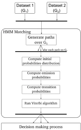
The pipeline of our method is depicted in Figure 2. The matching section is based on a HMM and driven by geometrical and topological criteria. Then, a decision making process is used to filter potential candidates and establish the final matching links.
Figure 2: Pipeline of the proposed HMM matching process.
2.2
States, observations, and paths
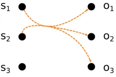
(a) (b)
Figure 3: (a): A path(o1, o2, o3)ofG1in red, with possible matching links depicted with dotted lines for each edgeoi. (b): The corresponding situation translated in a HMM repre-sentation.
Formally, in our matching algorithm, the observations are the edges of the first network
G1we want to match. The states are the edges of the second networkG2. Thus, a path is a cluster of observations and represents a walk in the graphG1. Each statesihas a probability to emit an observationoj representing how likely the matching of edgesi with edgeoj is. The goal of the HMM matching algorithm, given a sequence of observations, namely a path of consecutive edges ofG1, is to find the sequence of states associated with the observations, and therefore the edges ofG2matched with the edges of the path observed inG1.
Figure 4 depicts how the HMM works. Solid blue lines represent networkG2and dot-ted red ones represents a path in networkG1. As observations (edges of G1) are itera-tively processed, feasible sequence of candidate edges for matching are considered inG2 (dashed black arrows). In the third step, three observations (edges ofG1) have been pro-cessed resulting in three possible corresponding sequences of hidden states. In the last step, sequence number 1 has been dismissed because of a topological break. Finally, se-quence number 2 will be chosen because it has the maximum state sese-quence probability (less bends, less length difference, etc.). Associated matched edges ofG2are depicted in thick green lines in Figure 4.
We specify that we do not generate path forG2, thus the algorithm’s goal is not to match clusters of edges ofG1with clusters of edges ofG2which is a more an alternate result of the algorithm, but rather to find matching links between individual edges of the two networks.
2.3
Path generation
Figure 4: Philosophy of the HMM matching, from left to right. As the algorithm runs, feasi-ble paths on the second graph are successively considered. Finally, thanks to the topology of the networks, the most feasible path is found and individual matching links between homologous edges are built. Matching links are not drawn for clarity reasons as well as over path solutions that might be feasible.
covered, meaning that each observation belongs to at least one cluster. We do not impose here that the path generation should lead to a set of disjoint clusters and thus a partition of the set of edges. Then each edge may well belong to more than one path. In this context, the HMM algorithm could lead to cases where one observation could be associated with more than one hidden state. We use a post-process strategy, called the decision making process, to filter such particular cases.
Several path generation strategies might be considered, such as random paths or short-est paths between random vertices. The choice of a strategy is not relevant is this method-ological section as the only hypothesis we need to describe the HMM algorithm is that the whole network is covered such as each edge ofG1 belongs to at least one cluster of observations.
2.4
Probabilities of the model
candidates (emission probabilities), which both constitute a trade-off between feasibility of the paths and matching scores and features likeness, and 3) the initial state probabilities.
2.4.1 Emission probabilities
Given an observationoi and a statesj, we model the probability thatoi was emitted by sj with the probability pemit(oi → sj). Emission probability represents the likelihood of matching link between one edge ofG1 and one edge of G2 based on how they look alike: the more similar the two features, the higher the probability and the more likely the matching. This probability can be calculated regarding several criteria such as ge-ometrical distances (Haussdorf or Fréchet distances, for instance) or semantics compar-isons. For instance in Figure 5, if we consider only shape similarity, we expect to have
pemit(o1→s1)> pemit(o2→s1).
2.4.2 Transition probabilities
Transition probability is the key concept of our topology-driven approach. Given a con-tinuous pathp = (oi)i≤l on G1, each edgeoi is possibly matched with several edges of G2, and so is oi+1. But, as we mentioned earlier, the candidates for matching withoi+1 are strongly constrained by the topology of the networks and the feasibility of the cor-responding path inG2, and therefore by the previous states of the HMM which emitted
(o1, ..., oi). But as a HMM has the Markov property, the probability thatoi+1 is matched with a given edge ofG2only depends of the previous state of the model. Thereby, the tran-sition probabilityptrans(oi+1→sk|oi →sj)gives the probability thatoi+1is matched with
skknowing thatoiis matched withsj. For instance in Figure 5, we expect the probability ptrans(o2 →s2|o1 →s1)to be high because the topology of the network strongly defends this hypothetical matching.
2.4.3 Initial state probability distribution
As for a simple Markov model, HMMs also require an initial state distribution of proba-bilities(πi)such thatπi is the probability thatsi is the initial state of the model. Thus, in our application, πi represents the probability that si is matched with the first edgeo1 of the considered path. Instead of using a uniform distribution, we rather use the emission probability distribution associated with the first edgeo1of the first network, as done in [31]. In other words, we consider thatπi=pemit(o1→si).
2.5
Modeling multiple cardinality of matching links
In practice, 1:N, M:1, and to a lesser extent N:M matching relationships often occur like shown in Figure 6, because of morphological evolutions of the network through time, dif-ferences in level of detail, etc.
Figure 6: Two contemporary road networks (BDCarto from IGN in solid blue line and OpenStreetMap in brown dashed line) with a high difference of level of detail, which in-volves matching links of multiple cardinalities.
Formalized the way we have, transition probabilities can manage N:1 links through the calculus ofptrans(oi+1 → sj|oi → sj)representing the possibility foroiandoi+1 to be matched with the same edge ofG2sj.
the HMM (see Figure 7.b) and thus new emission and transition probabilities need to be calculated.
(a) (b)
Figure 7: Ifoiis potentially matched withs1,s2, ands3, then new candidates are consid-ered, illustrated with hyperedge (a), by grouping those edges when merging is possible. Thus, three new states are introduced in the HMM.
2.6
Solving the HMM
Given a sequence of observations inG1, several corresponding sequences of hidden states inG2are feasible. Solving the HMM consists in finding the sequence of states that maxi-mize the product of both emission and transition probabilities, and thus constitute the best compromise between similarity of matched edges and feasibility of the topological connec-tions between them. We use the Viterbi algorithm [44], based on dynamic programming, to find the most likely sequence of hidden states, and therefore inference the matched path onG2.
2.7
Dealing with expected unmatched entities
For the same reasons that N:M matching links occur, in practice several edges ofG1orG2 may have no counterpart in the other network. The HMM finds a corresponding object for all edges ofG1 as long as emission probabilities are never null. Thereby, it is likely that at the end of the HMM solving, some edges ofG1that should be unmatched have mutual matches inG2with other edges, and reciprocally, as depicted in Figure 8.
To deal with this situation, one could introduce geometric thresholds such as maximum distance in the emission probabilities computation to filter matching links. To avoid the use of thresholds, we explore two non-exclusive solutions.
2.7.1 Double HMM matching
Our first proposal is based on the consideration that, theoretically, the matching ofG1with
Figure 8: The circled matching links should not exist but are found by the HMM.
HMM finds that the observationoinG1has been emitted by the statesinG2, the reverse HMM should find that the observationsinG2is emitted by the stateoinG1.
We implement this principle with a double HMM matching (see Figure 9): edges of
G1are in a first step considered as the observation sequences, then as the hidden states of the HMM. This produces two sets of matching links and we only keep correspondences between edges that are matched in both cases (see Figure 10).
Figure 9: Principle of the double HMM matching approach.
(a) (b)
(c)
Figure 10: (a): Results of the matching ofG1withG2with HMM approach. (b): Results of the matching ofG2withG1with HMM approach. (c): Final results, thanks to the double HMM decision making process.
2.7.2 Assignment modeling of the decision making process
Our second solution considers the decision making process as an assignment problem with an additional hierarchical dimension. Indeed, in its most general form, the assignment problem aims at finding, in a weighted bipartite graph, a set of edges without common vertices in which the sum of weights of the edges is maximum. In the context of data matching, the vertices of the bipartite graph would be the entities we want to match, and its edges would represent potential matching links between two objects with a weight equal to the probability of the match. But, thus stated, the assignment problem is only suitable to deal with 1:1 correspondences. Thereby, we model the matching problem as a hypergraph assignment problem.
A hypergraph consists of a set of vertices and a set of hyperedges connecting vertices. So basically, a hypergraph is a graph in which edges can connect not just two vertices but any number. The cardinality of a hyperedge is the number of vertices it connects. A graph is simply a hypergraph in which the cardinalities of all edges is equal to 2.
We build the bipartite hypergraphHc= (Vc, Ec)as follows:
• The verticesVc=E1∪E2is the union of all edges ofG1andG2we want to match. • A hyperedge can connect any subset of edges ofG1with any subset of edges ofG2.
We build a hyperedge of cardinality 2 between each edge ofG1andG2to model 1:1 links. In order to model N:M matching links, we also build a hyperedge when one or several edges ofG1are matched with one or several edges ofG2, connecting the edges that have mutual candidates when the edges from the same network can be ge-ometrically merged. For instance, let’s assume we have the following matching links at the end of the HMM:(s1, o1, o2),(s2, o2, o3), and(s3, o1)as illustrated in Figure 11. Then, we create five hyperedges connecting the various matched edges, which gives
Those hyperedges represent matching links between edges wrapped together as new geo-metrically valid entities. It is thus possible to detect matching links with multiple cardinal-ity by choosing a single hyperedge ofHc.
(a) (b) (c)
Figure 11: (a): Potential matching links between pair of candidates are depicted in black dotted lines. (b): A graph representation of potential matching links between edges ofG1 and edges ofG2. (c): Hypergraph built from previous graph with hyperedges represented with single colors. Hyperedge(s1, s2, o1, o2, o3)is added to the hypergraph becauses1and
s2have mutual candidates we can geometrically merge.
Each hyperedge is weighted with a score computed as the emission probability of the merging of edges coming fromG1and the merging of those coming fromG2. The final de-cision making process then consists in the selection of a set of hyperedges fromHc which have no mutual vertices (edges ofG1and/orG2) and such as the sum of the weights of the selected hyperdeges is maximized. As far as we know, the resolution of the hypergraph assignment problem is still at a research state and there is no algorithm that could be eas-ily implemented to solve it. We propose to reduce it to a constrained linear optimization problem.
LetCbe the vector of scores such asceinC is the score of the hyperedgeeinEc. Let δ:Ec →0,1be the function indicating whether or not a hyperedge is selected in the final solution: δ(e) = 1ifeis chosen andδ(e) = 0otherwise. Finally, we noteV(v)the set of hyperedges that are incident to vertexv inVc. Thus, the assignment problem consists in the maximization of the objective function
X
e∈Ec
δ(e)ce (1)
under the following constraints:∀v∈Vc, Pe∈V(v)δ(e)≤1(all nodes cannot be linked with more than one selected hyperedge) and∀e ∈Ec, δ(e)∈ {0,1}. This solution can be used with the result of only one HMM as an input, and also with the matching links from the double algorithm introduced above.
3
Use cases and implementation
Figure 12: Solution of the assignment problem associated with the hypergraph 12.c, where hyperedges are weighted with simple distance between lines. The best choice here is to select only one hyperedge ((s1, s2, o1, o2, o3)), thus edges3is unmatched.
3.1
Datasets
To validate our approach, we use four heterogeneous datasets.
Streets The first set of data consists of geohistorical street networks extracted from two to-pographical maps of Paris, refereed as “Verniquet map” and “Jacoubet Atlas,” respectively created at the scale of1 : 8000between 1783 and 1799, and at the scale of1 : 2000between 1825 and 1837 [13]. The main imperfections and heterogeneities of these two networks challenging the matching process are geometrical discrepancies due to time difference and morphological evolution of Paris, and also the accuracies of the sources and differences of scales and levels of detail.
Roads The second dataset is contemporary road networks, one from BDCarto, a precise and homogeneous cartographic reference map produced by the French mapping agency at a medium scale (between1 : 50000and1 : 200000), and the other from OpenStreetMap with heterogeneous level of detail [42].
Railways The third dataset consists of railway networks from the same sources as the second dataset.
Hydrography Finally, the last dataset is composed of hydrographic networks from BD-Carto and BDTopo, another reference vectorial map produced by the French mapping agency at a lower scale (between1 : 5000and1 : 50000) and higher level of detail than BDCarto.
Table 1 summarizes the characteristics of our testing datasets.
3.2
Ground truth
To evaluate our approach, we use ~7000 checked and confirmed matching links of Paris street networks. This ground truth has been produced semi-automatically [8].
3.3
Preprocessing
topolo-Networks type Sources Main heterogeneities
Streets Verniquet Map (∼1790) Time difference. Level of detail and scale. Geometrical accuracy Jacoubet altas (∼1830)
Roads BDCarto Level of detail and scale. Geometrical accuracy OSM
Railways BDCarto Level of detail and scale.
OSM
Hydrography BDCarto Level of detail and scale.
BDTopo
Table 1: Network types and sources used to test our approach.
gies: very close nodes are clipped and duplicate nodes and edges are removed as well as suspicious very short edges.
3.4
HMM matching implementation
3.4.1 Path generation
In order to generate paths that cover the whole network, we arbitrarily choose a strategy which leads to a partition of the set of edges ofG1, i.e., each edge belongs exactly to one path. For this purpose, we use the “every best fits” algorithm from [24] that relies on an-gular criterion at junction point. The algorithm randomly chooses the first segment and iteratively choose for the next segment the one with the smallest deflection angle. This way generated clusters represent continuous objects based on the continuity principle of Gestalt. In order to avoid the introduction of a threshold for path length (number of edges in the path), we choose to keep small edges clusters. As each path can be processed inde-pendently of others, the implementation can easily be parallelized.
3.4.2 A selection threshold to speed-up the matching process
In their approach, Tong et al. [40] consider all possible pairs of matching candidates in order to avoid the use of selection thresholds. With complex and large datasets, such as city street networks, a risk of combinatorial explosion arises. Moreover, there is obviously no need to consider matching candidates that are quite distant one from the other. For that purpose, before the calculation of emission probabilities we introduce a selection threshold to filter distant candidates and help reducing the running time of our algorithm. This threshold may be calibrated according to our knowledge about the geometrical accuracy of considered datasets.
Figure 13: Impact of the selection threshold on F-score and computation time (4 replications for each selection threshold value).
3.4.3 Emission probabilities: measurement of features similarity
Recall that the emission probabilitypemit(oi→sj)is the probability that the observationoi has been emitted by the hidden statesjand measures how those features look alike. Many measures exists to quantify the similarity of linear features but we choose to adopt a purely geometrical and topological approach.
First of all, we intuitively assign higher probabilities to close features. Haussdorf dis-tance [1] or modified median Hausdorff disdis-tance are generally used, as presented in [40]. This approach computes distances from smallest line points to the longest line to avoid biases due to lines much longer than others. It may induce inconsistent matches with small orthogonal lines in dense areas like an urban center. Devogele [12] suggests to use the Fréchet distance instead (see Figure 14.a). According to the author, the Fréchet distance is more suitable because it also takes into account the shape of the polylines (see Figure 14.b). Thereby, we use a discrete partial Fréchet distanceδF, an approximation of the Fréchet distance calculated in polynomial time [14]. We could directly used the value of the Fréchet distance as emission probability, without introducing curve fitting parameters. But in order to better take into account the geometrical characteristics of the tested spatial networks, we rather look for a cost function more suitable than linear distribution. Figure 15 illustrates the cumulative distribution of the Fréchet distances based on our ground truth matched streets, and shows that it follows an exponential distribution with aR2of approximately 97%.
Thus the probability thatoiis matched withsjis given by:
(a) (b)
Figure 14: Computation of the Fréchet distance (a) and Hausdorff (δHon the figure) versus Fréchet (δF on the figure) distances (b) (image from http://dgtal.org).
Figure 15: Emission probability based on the Fréchet distance fits well an exponential dis-tribution.
3.4.4 Transition probabilities: modelling topological constraints
Let’s remember that the transition probability ptrans(oi+1 → sk|oi → sj) measures the probability that oi+1 is matched with sk knowing that its connected edgeoi is matched withsj.
We set to zero the probability of any transition(sj, sk)such assj andsk are not con-nected (see Figure 16 for edgessj andsp). This highlights the high constraint we impose with regard to topological relationships. In other cases, we promote transitions whose angle is similar to that betweenoiandoi+1.
Figure 16: As sj and sp are disconnected, we set to 0 the probability of the transi-tion ptrans(oi+1 → sp|oi → sj). Otherwise, it is possible to calculate the angles α1 =
](x1, x2, x3)andα2=](y1, y2, y3).
Sometimes, because multiple cardinality is possible for matching links, it may occur thatsj =sk. In such cases, we virtually splitskinto two new edges by projectingx2onsk. Then the new edges haven a common extremityy2(see Figure 17).
We denote byα1 = ](x1, x2, x3)the angle of the transition between the edges oi and oi+1, andα2 =](y1, y2, y3)the angle of the transition betweensj andsk. We refer as the trigonometric difference the counter-clockwise gap between two angleα1andα2, notated
δ(α1, α2). For instance,δ(
π/4 7π/4) =
3π
2. Finally, we compute the shortest difference between
α1andα2:θ(α1, α2) =min(δ(α1, α2), δ(α2, α1)). For instance,θ(π4,74π) =π2.
Figure 17: The computation ofα1 and α2, thus the transition probabilityptrans(oi+1 →
sk|oi→sj), is made possible by projectingx2onsk.
used an exponential probability distribution to fit the histogram of distance difference used as transition probability in their map matching approach. We also used our ground truth data to compute a histogram of angular difference between matched pair of streets (θ) as illustrated in Figure 18. This histogram follows an exponential distribution as well with a
R2of approximately 97%.
Figure 18: Transition probability based on angular difference fits well an exponential dis-tribution.
Then, the transition probabilityptrans(oi+1 →sk|oi →sj)representing the probability thatoi+1is matched withskknowing thatoiis matched withsjis given by:
ptrans(oi+1→sk|oi→sj) =βe−βθ(α1,α2)=βe−βmin(δ(α1,α2),δ(α2,α1)) (3)
3.5
Qualitative matching results for several types of networks
To run our tests, we arbitrarily usedλ = β = 1as parameters of the exponential distri-butions used as cost functions in the calculation of emission and transition probabilities. Qualitative analysis over a sample of matching results shows that the decision making process powered by the hypergraph assignment problem seems to produce better results in general, but differences are quite minimal. Figure 19 illustrates and example where the first decision making approach (double HMM) performs better at dealing with the differences of crossroads modelling (more detailed for Verniquet data) but also leads to false-positives (black circle). Red solid lines illustrate matching links between homologous edges.
We examined matching links produced by our algorithm for the four datasets. Globally, results are satisfying considering the facts that:
1. we use minimalistic, non-mandatory number of parameters to tune the algorithm: the selection threshold to filter matching pairs of candidates in order to speed up the process, and the type of the cost functions (exponential) for the calculation of emission and transition probabilities; and
(a) (b)
Figure 19: Sample results of HMM matching of Paris streets networks using our two post-process methods:
(a): double HMM method—black circle highlights a false-positive, and (b): hypergraph assignment problem method.
(a) (b)
Figure 20: Other sample results of HMM matching of Paris streets networks.
Our approach succeeds at matching several kinds of spatial networks with different hetero-geneities and imperfections. Figure 20 illustrates matching results on Paris street networks, and shows good quality of matchings, even for roundabouts 20(b) and despite geometrical discrepancies 20(a). Scores will be given for those datasets in the next section. Figure 21 highlights the robustness of HMM matching to deal with networks with heterogeneous lev-els of details (roads), whether between the two networks, or within one of them: matching is good in overall for countryside roads, and also for city roads and streets.
HMM matching also correctly deals with railways which are networks with different scales (see Figures 22 and 21). That involves a high selection threshold to take into account the potential large gap between candidates edges in the case of differences in the level of details of the datasets (i.e., to consider 1:N and N:M matching links). It is relevant to note that those networks have the specificity of not being wholly planar.
(a) (b)
(c)
Figure 21: Sample results of HMM matching of road networks with different scales and heterogeneous granularity:
(a): city streets,
(b): countryside road—black circle shows an example of false positive, and (c): a larger area.
intrinsic to the approach are due to its tendency to over-match features (see Figure 21.b). Indeed, as we do not use thresholds for each geometric criteria in the calculation of emis-sion probabilities, all edges ofG1 are possibly matched with one or several edges ofG2. Sometimes, the decision making process is not able to eliminate those false-positives.
3.6
Quantitative results and comparison with existing approach
Ground truth is used to calculate precision, recall and f-score which are measures conven-tionally used to evaluate a matching algorithm. Precision is the ratio of true positivestp
(correctly matched edges) over the sum of true positives and false positivesf p (wrongly matched edges) i.e. the total number of matchings: precision= tptp+f p. Recall is the ratio of true positives over the sum of true positives and false negativesf n(missing matchings):
recall= tp+tpf n.
Figure 22: Sample results of HMM matching of railway networks with different scales and level of detail.
algorithm is, whereas recall is a measure of completeness (to what extent does the algorithm miss matchings?). The F-score is a compromise between precision and recall.
Table 2 illustrates precision, recall, and F-score calculated for Paris street networks us-ing the HMM algorithm with both decision makus-ing process. The results are compared to Opt [27] approach which is a classical and performing algorithm for matching networks. We used optimal parameters for both algorithms, given by a calibration computed using the OpenMOLE platform [33, 34], such that F-score is maximized (see section 3.7).
Approach Precision Recall F-Score
Double HMM 94.60% 92.90% 93.74% HMM + optimization 93.57% 94.98% 94.27% Opt [27] 91.97% 95.83% 93.86%
Table 2: Quantitative evaluation of HMM algorithm on Paris street networks. Selection threshold,αandβare respectively set to 14, 50, and 23.6.
First of all, even though additional evaluation on other datasets should be achieved, these numbers allow us to draw the following conclusions:
(a) (b)
(c)
Figure 23: Results for hydrographic tree-like networks with different scales.
• Recall and precision values are almost equal. This highlights a balanced algorithm which tends to conciliate between two strategies: matching many objects in order to ensure that a maximum of expected matching links are actually found (high recall) with possibly low accuracy, and matching few objects with high accuracy even if it implies significant number of false negatives. Our approach appears to be more balanced than Opt [27] which is more optimistic (recall higher than precision). • As supposed in the qualitative analysis, the decision making process based on
(a)
(b)
Figure 24: Matching results using Opt [27] (a) and HMM algorithm (b). Green, red, and blue arrows are respectively true positives, false positives, and false negatives.
The HMM algorithm seems to perform better for datasets with different levels of detail, such as differences in the representation of intersections, as shown in Figure 24. Never-theless, the Fréchet distance might be insufficient in some cases to discriminate between several matching candidates. Figure 25.c shows the result of the HMM before the deci-sion making process. In this case, as several matching sets are topologically possible, it is mostly the emission probabilities that lead to the given solution. This issue could be overcome by choosing other measures or combinations of distances for the computation of emission probabilities. One significant strength of our approach is scalability. As each path can be processed independently of the others, our algorithm can be easily parallelized. On our desktop computer (Intel Core i5 @ 2.60GHz ; RAM 8Gb), the matching of Paris street networks took 45 seconds, whereas Opt [27] matching computation needed 23 minutes to complete, with data divided in 3 areas so that the optimization calculations could be completed without overflowing the RAM.
3.7
Algorithm exploration
Four parameters (α,β,pathMinLength,selectionThreshold) can be considered in our imple-mentation:
• the parameters of exponential distributions, modeling emission and transition prob-abilities (αandβ);
(a) (b)
(c)
Figure 25: Matching results on the data sample shows that HMM might miss matching links (a) despite topological criterion because the choice of the Fréchet distance is not dis-criminating enough, and (b) is the result of the HMM before the assignment optimization. In this case, Opt [27] performs better (c). Green, red, and blue arrows are respectively true positives, false positives, and false negatives.
that do not benefit from the topology-driven approach because then matching is only determined by emission probabilities. To our knowledge there are no studies of the least number of steps needed before convergence of the HMM to a single solution, that is to say, the number of transitions after which new observations do not impact the first match anymore. Thus, this parameter is relevant to look for an optimal path length (smaller paths involves worst results, and longer paths does not involve better results); and
• the selection threshold,selectionThreshold.
In order to better understand the sensitivity of the parameters of the proposed algo-rithm, we performed several explorations using the OpenMOLE platform [33, 34]. Open-MOLE is a free and open-source platform that offers tools to run, explore, diagnose, and optimize numerical models, taking advantage of distributed computing environments1. OpenMOLE offers different types of so-called Tasks designed to embed models. Tasks such asScalaTask,RTask, andNetLogoTaskare specific to a programming language whereas CARETaskandContainerTaskare designed to embed models written in other languages such as python or C. Once a model is embedded, OpenMOLE offers algorithms to design exper-iments. Such algorithms include sampling parameters, model calibration [37], incremental modelling [9], diversity search [6], and sensitivity analysis [35]. Finally, the experiments
designed with OpenMOLE can be delegated to a remote execution environment such as Slurm2[49], HTCondor3[39], or EGI4[16].
Figure 26: Calibration of the proposed algorithm using genetic algorithms. Color indicates the number of replications represented by each point of the calibration.
After integrating our algorithm into OpenMOLE (using aScalaTask), we performed a calibration using the ground truth presented in section 3.2. The results of this calibration (see Figure 26), using a multiple-criteria calibration with precision and recall, show that the algorithm searches for a compromise between these criteria. (There is no solution on the Pareto frontier where one criterion is clearly preferred over the other. In other words, the solutions are all grouped in a single cluster.)
After the calibration was finished, we selected the best parameter set using the F-score (see section 3.6) from the calibration results. 100 replications of this parameter set were then computed (see Figure 27) by modifying the randomseedparameter. Indeed, due to the stochastic nature of the algorithm, different results can be obtained using different ran-dom number generation sequences. The ranran-dom seed parameter allows us to initialize the random number generator in different ways. These results show that the variation of the F-score due to the stochasticity of the model is acceptable (with a standard deviation of approximately 0.15%). Finally, four calibration profiles [35] were computed in order to estimate the impact of each parameter on the results. These results show thatα,β, and pathMinLengthhave no significant effect on the results of the algorithm, and thus do not constitute parameters of the model and can be set to any random value (see Figure 28a for theαcalibration profile). TheselectionThresholdparameter is the only significant parameter and seems to have optimal values between10mand20mfor the tested network data (see Figure 28b).
Figure 27: Replication of the best calibrated solution with 100 replications.
4
Discussion and conclusion
Matching geographic features is a major step for many processes such as data qualifica-tion, integraqualifica-tion, and update. More particularly, for spatial networks that sustain critical infrastructures, matching allows to detect changes and helps with the understanding of the transformations and evolution of entities like cities or countries.
Most of linear object matching does not properly take advantage of the underlying topology of networks and frequently needs numerous parameters whose calibration is ei-ther unintuitive or tricky because of data imperfections and heterogeneities. Furei-thermore, published matching algorithms are mostly tested on street or road networks and never evaluated on different sorts of data with different types of imperfections.
(a)α
(b) selectionThreshold
Figure 28: Selected calibration profiles for the proposed algorithm. Color indicates the number of replications represented by each point of the calibration profile.
The HMM matching approach has been proved to perform well with the matching of four different types of networks (hydrography, railways, roads, and streets), even non pla-nar ones. It also correctly manages some major data heterogeneities (scale, level of detail, morphological evolutions) and imperfections (geometric accuracies). We also compared our results with those of Opt [27] and proved that the HMM algorithm performs slightly better in the case of Paris street network.
emission probability is positive, every edge is susceptible to be matched. Even if the double HMM matching or the assignment optimization correctly deal with expected unmatched objects, false positives may remain.
Several points merit further research. First, we used the Fréchet distance for the calcu-lation of emission probabilities in the implementation of the HMM. It would be useful to test and combine other type of distances that might perform better. Second, we used the “every best fits” algorithm to generate paths that cover the network. It might be interesting to compare the results of our approach using this algorithm with other path-generation strategies, such as random paths, or shortest paths between random vertices, to each other. In this paper, we also compared the results of the HMM algorithm with that of Opt [27]. It would be relevant to consider other well-tested approaches, and more generally to set up a systematic process which would compare the results of a new matching algorithm with those of validated literature approaches. Finally, we initialized state probabilities with the distribution of emission probabilities associated with the first edge of the path, as done in [31]. This way, the probability for any edge sito be matched with the first edgeo1of one path is fully given by the emission probabilitypemit(o1→si). An improvement might be to use manual matching instead, that is to say to ask the user to manually link the first edge of the path with its equivalent in the other network. This last point leads us to study the interest of developing an online version of the HMM matching [19] that would match on the fly a network under acquisition with a reference network.
Acknowledments
We thank the entire GeoHistoricalData team for their combined efforts in co-constructing open geohistorical data, Romain Reuillon, Mathieu Leclaire and the entire OpenMOLE team for their assistance in the exploration and calibration of the models used in the ar-ticle. We also thank the anonymous reviewers for their feedback and gratefully acknowl-edge the support of the French Agence Nationale de la Recherche (ANR), under grant ANR-18-CE38-0013 (SoDUCo project).
Code and data
The code used in this article is accessible at https://github.com/GeoHistoricalData/ HMMSpatialNetworkMatcher for the proposed algorithm and at https://github.com/ GeoHistoricalData/nm for the OpenMOLE plugin and Opt implementation. The data, containing ground truth, used for comparison between the algorithms, is available at https://dataverse.harvard.edu/dataset.xhtml?persistentId=doi:10.7910/DVN/CCESX4.
References
[1] ALT, H.,ANDGODAU, M. Computing the Fréchet distance between two polygonal curves.International Journal of Computational Geometry and Applications(1995).
[3] BAUM, L. E., AND PETRIE, T. Statistical inference for probabilistic functions of fi-nite state markov chains. The annals of mathematical statistics 37, 6 (1966), 1554–1563. doi:10.1214/aoms/1177699147.
[4] BERGE, C. Graphs, vol. 6. North-Holland, 1985.
[5] BOUCHON-MEUNIER, B. Aggregation and fusion of imperfect information, vol. 12. Phys-ica, 2013. doi:10.1007/978-3-7908-1889-5.
[6] CHÉREL, G., COTTINEAU, C.,ANDREUILLON, R. Beyond corroboration: Strengthen-ing model validation by lookStrengthen-ing for unexpected patterns. PLoS ONE 10, 9 (09 2015), 1–28. doi:10.1371/journal.pone.0138212.
[7] COSTES, B. Matching old hydrographic vector data from cassini’s maps.e-Perimetron 9, 2 (2014), 51–65.
[8] COSTES, B. Vers la construction d’un référentiel géographique ancien: un modèle de graphe agrégé pour intégrer, qualifier et analyser des réseaux géohistoriques. PhD thesis, Paris Est, 2016.
[9] COTTINEAU, C., CHAPRON, P., ANDREUILLON, R. Growing models from the bot-tom up. An evaluation-based incremental modelling method (ebimm) applied to the simulation of systems of cities. Journal of Artificial Societies and Social Simulation 18, 4 (2015), 9. doi:10.18564/jasss.2828.
[10] DE RUNZ, C., AND DESJARDIN, É. Towards a new typology of spatiotemporal im-perfection through a study of archaeological excavation data. InNinth International Symposium on Spatial Accuracy Assessment in Natural Resources and Environmental Sci-ences(Leicester, UK, July 2010).
[11] DEVOGELE, T.Processus d’intégration et d’appariement de bases de données Géographiques, Applications à une base de données routières multi-échelles. PhD thesis, Université de Ver-sailles, 1997.
[12] DEVOGELE, T. A new merging process for data integration based on the discrete Fréchet distance. In Advances in spatial data handling. Springer, 2002, pp. 167–181. doi:10.1007/978-3-642-56094-1_13.
[13] DUMENIEU, B. Un système d’information géographique pour le suivi d’objets historiques urbains à travers l’espace et le temps. PhD thesis, Paris, EHESS, 2015.
[14] EITER, T.,ANDMANNILA, H. Computing discrete Fréchet distance. Tech. rep., Chris-tian Doppler Laboratory for Expert Systems, TU Vienna, Austria, 1994. Tech. Report CD-TR 94/64.
[15] FAN, H., YANG, B., ZIPF, A., AND ROUSELL, A. A polygon-based ap-proach for matching OpenStreetMap road networks with regional transit authority data. International Journal of Geographical Information Science 30, 4 (2016), 748–764. doi:10.1080/13658816.2015.1100732.
[17] FISHER, P. F. Models of uncertainty in spatial data. Geographical information systems 1 (1999), 191–205.
[18] GLEYZE, J.-F. Using structural approach to understand transportation networks vul-nerability. InEuropean Geosciences Union 2008(2008).
[19] GOH, C. Y., DAUWELS, J., MITROVIC, N., ASIF, M., ORAN, A., AND JAILLET, P. Online map-matching based on hidden markov model for real-time traffic sensing applications. InIntelligent Transportation Systems (ITSC), 2012 15th International IEEE Conference on(2012), IEEE, pp. 776–781. doi:10.1109/ITSC.2012.6338627.
[20] GOODCHILD, M. F. Sharing imperfect data. InProceedings UNEP and IUFPRO inter-national workshop in cooperation with FAO in developing large environmental databases for sustainable development ,(1995).
[21] GOODCHILD, M. F. Combining space and time: new potential for temporal GIS. Plac-ing history: How maps, spatial data, and GIS are changPlac-ing historical scholarship (2008), 179–198.
[22] HAMMING, R. W. Error detecting and error correcting codes. Bell System technical journal 29, 2 (1950), 147–160. doi:10.1002/j.1538-7305.1950.tb00463.x.
[23] HUNTER, G. J. Managing uncertainty in GIS.Geographical information systems 2(1999), 633–641.
[24] JIANG, B., ZHAO, S.,AND YIN, J. Self-organized natural roads for predicting traffic flow: A sensitivity study. Journal of Statistical Mechanics: Theory and Experiment(July 2008). doi:10.1088/1742-5468/2008/07/P07008.
[25] LEVENSHTEIN, V. Binary codes capable of correcting deletions, insertions and rever-sals.Doklady Akademii Nauk SSSR 4(163)(1965,), 845–848.
[26] LI, L., AND GOODCHILD, M. Automatically and accurately matching objects in geospatial datasets. InProceedings of joint international conference on theory, data handling and modelling in geospatial information science(2010), pp. 26–28.
[27] LI, L.,ANDGOODCHILD, M. F. An optimisation model for linear feature matching in geographical data conflation.International Journal of Image and Data Fusion 2, 4 (2011), 309–328. doi:10.1080/19479832.2011.577458.
[28] LONGLEY, P. A., GOODCHILD, M. F., MAGUIRE, D. J., AND RHIND, D. W. Geo-graphic information system and science.England: John Wiley & Sons, Ltd(2001). [29] LÜSCHER, P., BURGHARDT, D., ANDWEIBEL, R. Matching road data of scales with
an order of magnitude difference. In23th International Cartographic Conference(2007). [30] MUSTIÈRE, S.,ANDDEVOGELE, T. Matching networks with different levels of detail.
GeoInformatica 12(2008), 435–453. doi:10.1007/s10707-007-0040-1.
[32] OLTEANURAIMOND, A.-M.,ANDMUSTIÈRE, S. Data matching—a matter of belief. Headway in Spatial Data Handling(2008), 501–519.
[33] REUILLON, R., CHUFFART, F., LECLAIRE, M., FAURE, T., DUMOULIN, N., AND HILL, D. R. Declarative task delegation in OpenMOLE. In High Performance Computing and Simulation (HPCS), 2010 international conference on (2010), pp. 55–62. doi:10.1109/HPCS.2010.5547155.
[34] REUILLON, R., LECLAIRE, M., AND REY-COYREHOURCQ, S. OpenMOLE, a workflow engine specifically tailored for the distributed exploration of simula-tion models. Future Generation Computer Systems 29, 8 (2013), 1981 – 1990. doi:10.1016/j.future.2013.05.003.
[35] REUILLON, R., SCHMITT, C., ALDAMA, R. D.,ANDMOURET, J.-B. A new method to evaluate simulation models: The calibration profile (CP) algorithm.Journal of Artificial Societies and Social Simulation 18, 1 (2015), 12. doi:10.18564/jasss.2675.
[36] SAMAL, A., SETH, S., AND CUETO, K. A feature-based approach to conflation of geospatial sources. InInternational Journal of Geographical Information Sciences(2004), vol. 18, pp. 459–489. doi:10.1080/13658810410001658076.
[37] SCHMITT, C., REY-COYREHOURCQ, S., REUILLON, R.,ANDPUMAIN, D. Half a billion simulations: Evolutionary algorithms and distributed computing for calibrating the simpoplocal geographical model.Environment and Planning B: Planning and Design 42, 2 (2015), 300–315.
[38] SHAFER, G.,ET AL.A mathematical theory of evidence, vol. 1. Princeton university press Princeton, 1976.
[39] THAIN, D., TANNENBAUM, T., AND LIVNY, M. Distributed computing in practice: the condor experience. Concurrency and Computation: Practice and Experience 17, 2–4 (2005), 323–356. doi:10.1002/cpe.938.
[40] TONG, X., LIANG, D.,ANDJIN, Y. A linear road object matching method for confla-tion based on optimizaconfla-tion and logistic regression.International Journal of Geographical Information Science 28, 4 (2014), 824–846. doi:10.1080/13658816.2013.876501.
[41] TONG, X., SHI, W.,ANDDENG, S. A probability-based multi-measure feature match-ing method in map conflation. International Journal of Remote Sensing 30, 20 (2009), 5453–5472. doi:10.1080/01431160903130986.
[42] TOUYA, G.,ANDREIMER, A. Inferring the scale of OpenStreetMap features. In Open-StreetMap in GIScience. Springer, 2015, pp. 81–99. doi:10.1007/978-3-319-14280-7_5.
[43] VANGENOT, C., PARENT, C.,ANDSPACCAPIETRA, S. Multi-representations and mul-tipleresolutions in geographic databases. Proceedings of the Advanced DatabaseSympo-sium" 99 (ADBS 99) 99, LBD-CONF-1999-009 (1999).
[45] VOLTZ, S. An iterative approach for matching multiple representations of street data. InIn Proceedings of ISPRS Workshop, Multiple representation and interoperability of spatial data(Hanovre (Allemagne), feb 2006), pp. 101–110.
[46] WALTER, V., AND FRITSCH, D. Matching spatial data sets : a statistical ap-proach. International Journal of Geographical Information Science 13:5 (1999), 445–473. doi:10.1080/136588199241157.
[47] WEST, D. B.Introduction to graph theory, vol. 2. Prentice hall Upper Saddle River, 2001.
[48] WU, Z.,ANDPALMER, M. Verb semantics and lexical selection. InIn Proceedings of the 32nd Annual Meetings of the Associations for Computational Linguistics(1994), pp. 133– 138. doi:10.3115/981732.981751.
[49] YOO, A. B., JETTE, M. A., AND GRONDONA, M. SLURM: Simple Linux Utility for Resource Management. InJob Scheduling Strategies for Parallel Processing(Berlin, Hei-delberg, 2003), D. Feitelson, L. Rudolph, and U. Schwiegelshohn, Eds., Springer Berlin Heidelberg, pp. 44–60. doi:10.1007/10968987_3.
[50] YUAN, S.,ANDTAO, C. Development of conflation components.Proceedings of Geoin-formatics, Ann Arbor(1999), 1–13.