Visual Function in Glaucoma: improving
the assessment of computerised visual
fields
Ananth Chitur Viswanathan
Submitted in fulfilment of the requirements
for the degree of Doctor of Medicine
Institute of Ophthalmology
University College
ProQuest Number: U641903
All rights reserved
INFORMATION TO ALL USERS
The quality of this reproduction is dependent upon the quality of the copy submitted.
In the unlikely event that the author did not send a complete manuscript and there are missing pages, these will be noted. Also, if material had to be removed,
a note will indicate the deletion.
uest.
ProQuest U641903
Published by ProQuest LLC(2015). Copyright of the Dissertation is held by the Author.
All rights reserved.
This work is protected against unauthorized copying under Title 17, United States Code. Microform Edition © ProQuest LLC.
ProQuest LLC
789 East Eisenhower Parkway P.O. Box 1346
Abstract
Glaucoma is a leading cause of world blindness. In order to ascertain whether the
disease is progressive or stable, glaucoma patients’ visual function is monitored at
regular intervals by testing the visual field using the technique of automated
perimetry. The numerical data obtained, relating to the spatial co-ordinates of the
test locations and light sensitivities at those locations, are amenable to sophisticated
statistical analysis.
This thesis centres on a method for detecting glaucomatous change in serial visual
fields known as pointwise linear regression: univariate linear regression of
sensitivity on time is performed for each test location in the visual field. This
method has been incorporated into a software package, PROGRESSOR.
Results indicate that PROGRESSOR is superior to previously accepted glaucoma
change probability software in the early detection of glaucomatous visual
deterioration. A higher level of concordance between expert observers in the
assessment of glaucomatous visual progression is found when PROGRESSOR,
rather than standard clinical methods, is used.
The optimum frequency of visual field testing is investigated: reducing the
frequency of examinations from 3 per year to 1 per year results in failure to detect
over half of the deteriorating test locations.
A strong association is found between patient perception of visual disability and
objectively measured damage and deterioration in glaucomatous visual fields even
Image processing techniques have previously been used to increase the
reproducibility and predictability of automated visual field tests. These techniques
are incorporated into PROGRESSOR. Results presented in this thesis indicate that
these benefits are obtained without delayed detection of visual field progression.
The PROGRESSOR software shows great potential in the detection and
quantification of glaucomatous visual field deterioration. It promises to be an
Table of Contents
Title p a g e ...1
A bstract...2
Table of Contents... 4
List o f T ables... 8
List o f Figures...9
Key o f Abbreviations... 11
Acknowledgements... 12
CHAPTER 1. INTRODUCTION... 13
1.1 G laucom a...13
1.1.1 Definition and classification...13
1.1.2 A etiology... 14
1.1.2.1 Mechanical theory... 14
1.1.2.2 Vascular theory...15
1.1.3 Epidemiology... 16
1.1.3.1 Prevalence... 16
1.1.3.2 Incidence... 17
1.1.3.3 Risk factors... 17
1.1.3.3 (i) A g e... 17
1.1.3.3 (ii) Intraocular pressure... 18
1.1.3.3 (iii) R a c e ... 18
1.1.3.3 (iv) Family history...19
1.1.3.3 (v) Other factors... 19
1.1.4 Treatm ent...20
1.1.4.1 Medical therapy... 20
1.1.4.2 Laser therapy... 20
1.1.4.3 Surgical therapy... 21
1.2 Visual Field A nalysis...21
1.2.1 Fundamentals of perim etry... 21
1.2.2 Development and history...22
1.2.2.1 Early perim etry... 22
1.2.2.2 Kinetic perim etry...22
1.2.3 Automated perim etry... 26
1.2.3.1 D evelopment...26
1.2.3.2 Static testing...26
1.2.3.2 (i) Full threshold strategies... 26
1.2.3.2 (ii) Suprathreshold strategies... 28
1.2.3.2 (iii) Full threshold versus suprathreshold strategies... 28
1.2.4 Humphrey Field Analyzer...29
11.2.4.1 Test patterns...30
! 1.2.4.2 Graphical display of re su lts...31
11.2.4.2 (i) Numerical threshold d a ta ... 31
11.2.4.2 (ii) Gray scales... 32
11.2.4.3 Global indices...34
11.2.4.4 The Glaucoma Hemifield Test...37
1.3 Change in visual fie ld ... 37
1.3.1 Measurement of change... 37
1.3.1.1 Automated versus manual perim etry... 37
1.3.1.2 Clinical judgement versus numerical analysis...38
1.3.1.3 Summary m easures... 38
1.3.1.4 Pointwise measures... 39
1.3.1.4 (i) Statpac 2 ...40
1.3.1.4 (ii) PROGRESSOR...41
1.3.1.4 (iii) Comparison of event analysis and trend analysis...43
1.3.2 Errors in measurem ent... 45
1.3.2.1 Fluctuation... 45
1.3.2.2 Learning e ffects... 46
1.3.2.3 Change criteria...47
1.3.2.4 Frequency of testing... 48
1.3.2.5 A rtefact...49
1.3.2.5 (i) Pupil size...49
1.3.2.5 (ii) Refractive erro r...49
1.3.2.5 (iii) Lid / brow artefact... 50
1.3.2.5 (iv) M edia opacities...50
1.3.2.5 (v) Macular disease...51
1.3.2.6 Reliability... 51
1.3.2.7 Dynamic range... 52
1.3.3 Results of treatm ent...52
CHAPTER 2. FREQUENCY OF VISUAL FIELD TESTING...54
2.1 A bstract...54
2.2 Introduction... 55
2.3 Materials and m ethods... 56
2.3.1 Subjects... 56
2.3.2 Testing strategy... 57
2.3.3 Progression criteria...57
2.3.4 Detection of progression... 58
2.3.5 ‘Thinning’ the fie ld s...58
2.3.6 Statistical analysis...58
2.4 Results... 60
2.4.1 Ability to detect progression...60
2.4.2 Detection tim e s... 60
2.5 Discussion... 64
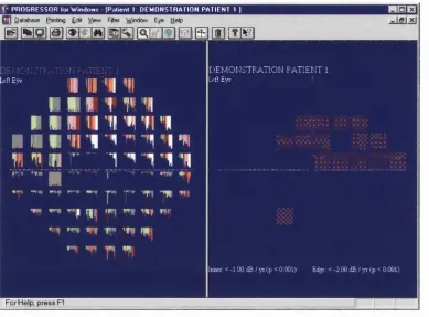
CHAPTER 3. PROGRESSOR FOR W INDOW S... 66
3.1 Bilateral display...66
3.2 Status bar information...67
3.3 M agnification... 67
! 3.4 Progressing points... 68
3.5 Subset analysis... 69
13.6 Progression indices... 70
3.8 Binocular simulation... 71
13.9 Help system... 73
CHAPTER 4. VALIDATION OF PROGRESSOR... 74
4.1 PROGRESSOR compared with Statpac 2 ...74
4.1.1 A bstract... 74
4.1.2 Introduction... 75
4.1.3 M eth o d s... 76
4.1.3.1 Subjects...76
4.1.3.2 Testing strategy...76
4.1.3.3 Progression criteria... 77
4.1 .3.3(i) Glaucoma Change Probability: Statpac 2 ...77
4.1.3.3(ii) PROGRESSOR... 77
4.1.3.4 Detection tim e... 77
4.1.3.5 Reliability of early detection... 78
4.1.3.6 Statistical analysis...78
4.1.4 Results... 79
4.1.4.1 Detection tim es...79
4.1.4.2 D elay... 80
4.1.4.3 Reliability...81
4.1.5 Discussion... 82
4.2 PROGRESSOR compared with standard clinical m ethods... 84
4.2.1 A bstract... 84
4.2.2 Introduction...85
4.2.3 M eth o d s... 87
4.2.3.1 Selection of visual field data... 87
4.2.3.2 Analysis of visual field data... 88
4.2.3.3 Statistical analysis...89
4.2.4 Results... 90
4.2.5 D iscussion... 95
CHAPTER 5. PATIENT PERCEPTION OF VISUAL FIELD STATUS... 98
5.1 A bstract...98
5.2 Introduction... 100
5.2.1 Severity of visual field damage... 100
5.2.2 Rate of visual field progression... 102
5.3 M eth o d s...103
5.3.1 Severity of visual field damage... 103
5.3.2 Rate o f visual field progression... 104
5.3.3 Statistical analysis... 105
5.4 Results... 106
5.4.1 Severity of visual field damage... 106
5.4.2 Rate of visual field progression... 107
5.5 D iscussion... 109
CHAPTER 6. SPATIAL FILTERING: IMPROVING REPRO D U CIBILITY 112 6.1 A bstract... 112
6.2 Introduction... 114
6.3 M eth o d s...115
6.3.2 Testing strategy...115
6.3.3 Progression criteria... 116
6.3.4 Detection tim e... 116
6.3.5 Spatial filtering...116
6.3.6 Statistical analysis... 117
6.4 Results...118
6.4.1 Detection tim e s...118
6.4.2 Number of progressing points at detection tim e... 119
6.4.3 Mean slope (whole field) at detection tim e ...119
6.4.4 Mean slope (progressing points) at detection tim e ...119
6.5 D iscussion... 121
CHAPTER 7. DISCUSSION...123
7.1 W ork to d a te ...123
7.2 Future w ork... 124
7.2.1 Frequency of visual field testing...124
7.2.2 Quality of life... 125
7.2.3 Image processing of visual field data... 126
7.2.4 PR O G R ESSO R ...126
7.4.1 Softw are... 127
7.4.2 A nalysis... 127
R EFER EN C ES...128
APPENDIX A. PROGRESSOR SOURCE C O D E ...143
APPENDIX B. SUPPORTING PUBLICATIONS... 365
Peer reviewed publications... 365
Papers under review ... 365
List of Tables
T a b l e 2.1 Tim eso fv is u a lf iel dt e st siny e a r sfr o mb a s e l in e...57
T a b l e 2 .2 Co n t in g e n c yt a b l efo rt h ep e r f o r m a n c eo ft h e ‘t h in n e d’ f i e l d s... 6 0 T a b l e 2 .3 Co m p a r is o no fd e t e c t io ntim e sb e t w e e nc o m p l e t ea n d ‘t h in n e d’ fields
(WiLcoxoN S ig n e d R a n k Z t e s t ) ...62
T a b l e 4.1.1 D e t e c t i o n t im e s f o r PROGRESSOR a n d S t a t p a c 2 ...79
T a b l e 4.2.1 Cl a s s m c a t io no ffiel dse r iesu s in g Hu m p h r e y Pr in t o u t s...9 0 T a b l e 4.2.2 C l a s s m c a t i o n o f f i e l d s e r i e s u s i n g PROGRESSOR... 91
Ta b l e 4 .2 .3a Co n c o r d a n c eb e t w e e no b s e r v e r sw h e nu s in g Hu m p h r e yp r in t o u t s...9 3 Ta b l e 4 .2 .3b Co n c o r d a n c eb e t w e e no b s e r v e r sw h e nu s in gPROGRESSOR...9 3 T a b l e 5.1 V i s u a l d i s a b i l i t y q u e s t i o n n a i r e ...103
Ta b l e 5 .2 Qu e s t io n sa s s o c ia t e dw ith Es t e r m a n Disa b il it y Sc o r e...107 T a b l e 5 .3 Asso c ia t io nb e t w e e np e r c e iv e dp r o g r e s s io na n dm e a s u r e dp r o g r e s s io nin
EITHER EYE... 108 T a b l e 5 .4 Asso c ia t io nb e t w e e npe r c e iv e dp r o g r e s s io na n dm e a s u r e db in o c u l a r
List of Figures
Fi g u r e s 1 .1aa n d b. Th e Go l d m a n npe r im b t e r (In t e r z e a g A G , Sc h l ie r e n, Sw it z e r l a n d). . 23 Fi g u r e s 1 .2a, ba n d c. Dia g r a mo fkin etics t r a t e g ya n dth ec o n s t r u c t io no fa nis o p t e r. 25 Fi g u r e 1 .3 . Dia g r a mo f 4 -2 d e c ib e l ‘tw or e v e r s a ls t a ir c a s e’ b r a c k e t in gs t r a t e g y 2 7 Fi g u r e 1 .4 Hu m p h r e y Fiel d An a l y z e r 6 3 0
(Hu m p h r e y In s t r u m e n t s In c., Sa n Le a n d r o, C A )... 3 0 Fi g u r e 1 .5 Hu m p h r e y Fiel d An a l y z e rr a ws e n sit iv it ypl o t (2 4 -2 s t r a t e g y) ... 3 2 Fi g u r e 1.6a Hu m p h r e y Fiel d An a l y z e rg r a ys c a l ed e r iv e df r o mt h en u m e r ic a lo u t p u t
OF Fig u r e 1 . 5 ... 33 Fi g u r e 1 .6b Hu m p h r e y Fiel d An a l y z e rg r a ys c a l el e g e n d... 3 4 Fi g u r e 1 .7 Ex a m p l eo fase c t io no fth e St a t p a c 2 Gl a u c o m a Ch a n g e Pr o b a b il it y
a n a l y s is. Th et e s tl o c a t io n s c ir c l e dinb l u ea r el a b e l l e da ssh o w in gs ig n if ic a n t d e t e r io r a t io nint w oo u to ft h et h r e efie l d ss h o w n. Th et e s tl o c a t io nc ir c l e din
RED IS l a b e l l e d AS SHOWING SIGNIFICANT DETERIORATION IN EACH OF THE THREE
CONSECUTIVE FIELDS...41 Fi g u r e 1 .8a Ex a m p l eo ft h e P R O G R E SSO R o u t p u tfo rt h es a m ev is u a lfiel ds e r ie sa sin
Fig u r e 1.7. Th eleftp a n es h o w st h ec u m u l a t iv eg r a p h ic a lo u t p u ta n dt h er ig ht p a n esh o w st h et e s tl o c a t io n sw h ic hsa t is f yp r o g r e ssio nc r it e r ia. No t et h a tt h e
PATTERN OF PROGRESSING POINTS IS SIMILAR TO THAT OF THE CIRCLED POINTS IN FIGURE 1.7 4 2 Fi g u r e 1 .8b P R O G R E S S O R l e g e n d. Thisl e g e n dr e l a t e sth ec o l o u ro fag iv e nb a rin
THE P R O G R E S S O R b a rg r a p h stoth epv a l u eo fth er e g r e s s io nsl o p efo rt h a t
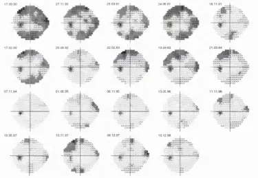
TEST... 4 3 Fi g u r e 1 .9 A se r ie so fv is u a lfiel d ssh o w in gt h ep e r s is t e n c eo fl e a r n in ge f f e c t so v e ra
PERIOD OF 8 YEARS... 4 6 Fi g u r e 1 .1 0 P R O G R E S S O R o u t p u tfo rt h es a m ev is u a lfiel dse r ie sa ss h o w n in
Fig u r e 1.9. Th ep r o g r e s s iv e l ysh o r t e n in gg r e e nb a r s in d ic a t eim p r o v e m e n tin
SENSmVITY OVER TIME, WHICH IN THIS PATIENT IS ATTRIBUTABLE TO LEARNING EFFECTS... 4 7 Fi g u r e 2 .1 De t e c t io nt im e sforc o m pl e t ea n d ‘t h in n e d’ v is u a lf ie l d s... 61 Fi g u r e 2 .2 Hist o g r a m o fd e l a yind e t e c t io no fp r o g r e s s in gp o in t su s in g ‘t h in n e d’
VISUAL FIELD TESTS...6 2 Fi g u r e 2 .3 Ea r l ie s td e t e c t io ntim e sfo re a c hp a t ie n t...63 Fi g u r e 3 .1 Sim u l t a n e o u sd is p l a yo ft h er e s u l t so fa n a l y s isf r o me a c he y eo fas u b j e c t. 6 7 Fi g u r e 3 .2 Cu m u l a t iv eg r a p h ic a ld is p l a yaf t e rm a g n ih c a t io no fac e n t r a lt e s t
LOCATION...6 8 Fi g u r e 3 .3 Pr o g r e s s io nc r it e r iad ia l o gb o x...6 9 Fi g u r e 3 .4 Da t ese l e c t io nd ia l o gb o x...7 0 Fi g u r e 3 .5 Pr o g r e s s io nin d ic e sd ia l o gb o x... 7 0 Fi g u r e 3 .6 Ane x a m p l eo f Ga u s s ia nfilt er in g. Th eleftp a n es h o w st h eu n f il t e r e d
P R O G R E S S O R ANALYSIS. Th erig h tp a n es h o w st h es a m ev is u a lfiel dse r ie sa f t e r
THE FILTER HAS BEEN APPLIED. THE PROGRESSING LOCATIONS IN THE SUPERONASAL AREA OF THE FIELD APPEAR TO DECAY MORE REGULARLY AND TO REACH HIGH STATISTICAL
SIGNIFICANCE (AS SHOWN BY WHITE BARS, P < 0 .0 0 1 ) SOONER AFTER FILTERING HAS BEEN PERFORMED...71 Fi g u r e 3 .7 Bin o c u l a rsim u l a t io nd is p l a y. Th elefta n dm id d l ep a n e ss h o wg r a y s c a l e s
FOR LEFT AND RIGHT EYES RESPECTIVELY. THE RIGHT PANE SHOWS THE RESULTS OF
BINOCULAR SIMULATION...7 2 Fi g u r e 3 .8 Bin o c u l a rs im u l a t io nd is p l a yid e n t ic a ltot h a ts h o w nin Fig u r e 3 .6 e x c e p t
THAT POINTS IN THE BINOCULAR SIMULATION WITH A SENSITIVITY OF LESS THAN 10 DECIBELS AND A BLUE RING CORRESPONDING TO THE CENTRAL 2 0 DEGREES OF THE VISUAL FIELD ARE SHOWN... 7 3 Fi g u r e 4 .1 .1 Dr o p-lin eg r a p ho fd e t e c t io ntim e sfo re a c hfiel dse r ie sfo r
P R O G R E S S O R AND STATPAC 2. Thefieldse r ie sa r er a n k e dino r d e ro fd e t e c t io n
Fi g u r e 4 .1 .2 Hist o g r a mo fd e l a yind e t e c t io na s s o c ia t e dw it h St a t p a c 2. Th em e a n
DELAY IS 1.085 YEARS (S.D. 0 .9 3 6 YEARS)...81 Fi g u r e 4 .2 .1 We ig h t e dk a p p av a l u e so fa g r e e m e n tf o ra l lt e npa ir so fo b s e r v e r s. Ea c h
PAIR IS REPRESENTED BY AN OPEN SYMBOL REPRESENTING THE WEIGHTED KAPPA VALUE WHEN USING H u m p h r e y p r i n t o u t s a n d a c l o s e d s y m b o l w h e n u s i n g PROGRESSOR.
Th epa ir sa r er a n k e da l o n gth ex-a x isb ym a g n it u d eo ft h ew e ig h t e dk a p p av a l u e. In a l l c a s e s t h e w e i g h t e d k a p p a v a l u e o f a g r e e m e n t w a s h i g h e r w h e n o b s e r v e r s
USED PROGRESSOR COMPARED TO WHEN USING HUMPHREY PRINTOUTS. THE RANGE OF
STANDARD ERROR FOR ALL THE WEIGHTED KAPPA VALUES WAS 0 .0 8 TO 0 .1 4 ... 9 2 Fi g u r e 5 .1 Ex a m p l eo fap r in t o u to fa Hu m p h r e y Fiel d An a l y z e r Es t e r m a ns t r a t e g y
Key of Abbreviations
A LT? Argon laser trabeculoplasty
dB Decibel
lOP Intraocular pressure
LF Long-term fluctuation
MD Mean deviation
MRI Magnetic resonance imaging
NTG Normal tension glaucoma
OHT Ocular hypertension
POAG Primary open-angle glaucoma
SD Standard deviation
SE Standard error
SF Short-term fluctuation
Acknowledgements
I gratefully and wholeheartedly acknowledge the guidance and support of my
supervisors Professor Fred Fitzke and Professor Roger Hitchings. I sincerely thank
them for actively directing my research and supporting my investigation o f areas of
interest.
I would like to express my thanks to my colleagues who collaborated in this
research;
• Dr. David Crabb for statistical advice and for collaboration in the research
described in Chapter 4.2 and Chapter 5.
• Mr. Andrew McNaught for collaboration in the research described in Chapter
4.2 and for collaboration and much of the data collection in the research
described in Chapter 5.
• Mr. M ark Westcott, Miss Deborah Kamal and Mr. David Garway-Heath for
collaboration in the research described in Chapter 4.2.
• Mr. Darmalingun Poinoosawmy and Dr. Luigi Fontana for collaboration in the
research described in Chapter 5.
I am deeply indebted to the International Glaucoma Association, particularly Mr.
Ronald Pitts Crick and Mr. David Wright, for the generous funding and travel grant
provisions I received as an International Glaucoma Association Fellow while the
research described in this thesis was being undertaken.
I thank Mr. Chris Jubb for invaluable technical help during the research described
in this thesis.
CHAPTER 1. INTRODUCTION
1.1 Glaucoma
1.1.1 Definition and classification
The term ‘glaucoma’ encompasses a group of pathological conditions which is
distinguished by characteristic patterns of damage to the optic nerve head with
concomitant abnormalities of the visual field. The visual field is defined as that
portion of space in which objects are simultaneously visible to the steadily fixating
eye.(l) Intraocular pressure (TOP) greater than 21mmHg (conventionally taken as
two standard deviations above the population mean(^)) is an important
characteristic of glaucoma, but raised TOP is neither a necessary nor a sufficient
condition for the diagnosis of glaucoma. It is reasonable, however, to suggest that
glaucoma is often, but not always, associated with a raised lOP.(^)
Glaucoma may be classified into primary and secondary types. In the majority of
cases, glaucoma is unrelated to other ocular or systemic disease and is considered
primary, whereas secondary glaucomas are related to conditions such as ocular
trauma or inflammation. Primary glaucomas are further classified according to the
appearance of the aqueous drainage angle on gonioscopy. If, in a case of glaucoma,
the angle is obscured by normal or pathological structures, a diagnosis o f closed-
angle glaucoma is made: otherwise the diagnosis is open-angle glaucoma. The
congenital glaucomas are a comparatively rare sub-group characterised by
malformations of the aqueous drainage structures with or without other ocular and
systemic congenital anomalies.
The commonest form of glaucoma in the UK is primary open-angle glaucoma
(POAG). A substantial minority of POAG patients (around 15% in population
based studies) consistently demonstrate intraocular pressures within the normal
glaucoma (NTG). Subjects who have normal visual fields but have risk factors for
the development of POAG, such as raised IGF or optic nerve head damage, are
typically described as ‘POAG suspects’ since they are at risk of developing POAG
in the future. Another classification term is ‘ocular hypertension’ (OHT). This
refers to individuals with raised lOP in the absence of visual field or optic disc
damage.
Untreated POAG leads to progressive irreversible visual loss. Although lO P
measurement and evaluation of the optic nerve head are very important in the
diagnosis and classification of POAG, it is visual field examination which provides
the best continuing measure of a POAG patient’s disease status and the best
measure of the functional impact of the disease, or of any therapy.
1.1.2 Aetiology
The pathophysiology of POAG is not fully understood. The two main theories to
account for the retinal nerve fibre loss seen in glaucoma are the mechanical theory
and the vascular theory. The mechanical theory proposes that increased lOP results
in direct nerve fibre damage, whilst the vascular theory suggests that an
abnormality in blood flow to the optic nerve head is the main cause of this
damage. (5)
1.1.2.1 Mechanical theory
The hypothesis that glaucomatous optic neuropathy is produced mechanically by
raised lOP was first stated by von Graefe in 1 8 5 7 . Experimentally-induced lO P
elevation in primates has been found to produce optic nerve head damage and loss
of visual function.(^ Quigley has stressed the primary role of raised lOP in the
pathogenesis of glaucomatous optic neuropathy, postulating that the characteristic
patterns of visual field damage observed in glaucoma result from regional
differences in the structure of the scleral lamina cribrosa and hence differing
susceptibility of nerve fibres to mechanical damage as they pass through this
Both mean and maximum lOP have been reported as closely associated with visual
field deterioration( 10-17) ^nd optic nerve damageX^^) In a group o f NTG subjects
worse visual field damage was found in the eye with the higher lOPX^^) However,
other studies have failed to demonstrate an unequivocal relationship between lOP
and loss of visual function(^^-^^) and have reported only moderate levels of within-
subject correlation between asymmetrical lOP levels and correspondingly
asymmetrical visual field d a m a g e .(23 24)
1.1.2.2 Vascular theory
In 1858 Jaeger put forward the hypothesis that damage to the optic nerve head in
glaucoma was the result of impaired circulation in the short posterior ciliary
arteries.(25) The degree of association between systemic arterial blood pressure and
glaucoma has recently been investigated.(26 27) Progressive visual field
deterioration in the face of lOP levels within the normal range was associated with
lower systemic arterial blood pressure than controls, and with relative nocturnal
hypotension. It is postulated that vascular risk factors cause hypoperfusion of the
optic nerve head leading to glaucomatous damage. Peripheral vasospasm(28) and
spontaneous platelet aggregation(29) have also been implicated in the pathogenesis
of glaucoma. The results of indirect techniques such as pulsatile ocular blood flow
measurement(50) and colour Doppler ultrasonography(51) have been used to infer a
disturbance of normal ocular blood flow in NTG. The response o f NTG patients to
systemically administered calcium channel antagonists(52 33) suggests that vascular
mechanisms are important role in the development of NTG.
It is likely that glaucomatous optic neuropathy occurs not as a result of purely
mechanical or purely vascular factors but rather from a combination of both. It may
be that there are subpopulations within the glaucomatous population in which
1.1.3 Epidemiology
At present glaucoma is the third commonest cause of blindness in the world/^^) It
will be the commonest cause of irreversible blindness by the year 2000/^^) It is
estimated that approximately 5.2 million people are bilaterally blind from
glaucoma: this represents 15% of the total burden of world blindness.(^^) There are
approximately 250,000 known sufferers in the UK and it is likely that an equal
number o f cases remain undiagnosed.(^^) With the shift towards an older
population the medical, social and economic burdens imposed by glaucoma are
likely to increase.
1.1.3.1 Prevalence
An early landmark in the epidemiological investigation of POAG was the Ferndale
study.(^) This study was notable because a large proportion of a geographically
defined population was examined using comprehensive case-finding methods and
extensive visual field testing. From the 4231 subjects studied (age range 40-70
years) a prevalence of POAG of 0.5% was obtained. In the Framingham Eye study
a sample of 2631 (age range 52-85 years) of the 3977 members o f the Framingham
(Massachusetts) Heart study population still living in 1973-1975 underwent
ophthalmological examinations for cataract, glaucoma, diabetic retinopathy,
macular degeneration and visual a c u i t y .(^9) The prevalence of POAG was found to
be 1.4%. A longitudinal study of 1511 (age range 55-70 years) of the 1963 residents
of a Swedish rural and suburban district using visual fields, ophthalmoscopy, slit-
lamp and tonometry gave an initial prevalence of POAG of 0.9%.(^0)
Three later studies, however, have suggested a higher prevalence of POAG. The
Roscommon study, set in a rural community in the W est of Ireland, was based on
evaluating multiple risk indicators including optic nerve head assessment, visual
fields and medical history, in addition to IOP.(^^) A total of 2186 people over the
age o f 50 were examined which represented a 99.5% response rate. The high
response rate was achieved by the community basis of the study and vigorous
prevalence of blindness amongst all POAG patients was 7.3%. The Baltimore Eye
Survey (41) in which 2395 black and 2913 white subjects aged 40 years or older
from the eastern and south-eastern health districts of Baltimore were studied gave
similar estimates of prevalence to the Roscommon study. The Beaver Dam Eye
study(42) conducted in Wisconsin on a sample of 4926 subjects (aged 43 years or
older) found the overall prevalence of POAG to be 2.1%. Despite differences in
examination method and diagnostic criteria for POAG these three recent studies
show remarkable concordance in prevalence of POAG against covariates of both
age and gender.
A recent meta-analysis of glaucoma prevalence data has stressed the importance of
a functional test of the visual field as part of the diagnostic criteria for POAG and
excluded studies based on measurement of lOP alone.(43)
1.1.3.2 Incidence
Direct measurement of the incidence of POAG is hampered by uncertainty over the
definition of an incident case: in a particular case the characteristic morphological
changes in the optic nerve head and retinal nerve fibre layer may, or may not
coexist with repeatable visual field loss(44). The incidence of manifest glaucoma
has been estimated for the age band 55-69 years by means of repeated automatic
perimetry in a defined general population from a small community in Sweden. It
was estimated at 0.24% per year.(45) Further estimates should arise from the
Baltimore and Beaver Dam Eye studies as more longitudinal data accumulates.
1.1.3.3 Risk factors
Since the precise causative mechanisms of POAG are unknown there is no clear cut
distinction between aetiology and risk factors. Nevertheless, several
epidemiological studies have found demographic, ocular and systemic attributes
which predispose an individual to POAG.
Age appears to be a primary risk factor for POAG. The Beaver Dam Eye study
reported a prevalence of POAG of 0.9% in subjects 43 to 54 years of age: this rose
to 4.7% in people aged over 75 y e a r s .(^2) The Roscommon study showed a four and
one half times increased risk of POAG in the 70-79 year old age group as compared
to the 50-59 age g r o u p . T h e Baltimore Eye Survey found an eightfold increase
for the same age groups.(^l)
1.1 .3 3 (ii) Intraocular pressure
Aside from being one of the putative mechanisms of glaucomatous damage (see
section 1.1.2.1) lOP is a major risk factor for POAG. Although only a small
number of patients with OHT develop POAG every year, studies on the conversion
from OHT to POAG have demonstrated that the overall risk of developing POAG
is approximately five times higher in subjects with lOPs greater than 21mmHg than
in subjects with lower IOPs(^^) and that the higher the lOP at screening, the greater
the risk of POAG.(^)
1.1.3.3 (iii) Race
Black Americans are at higher risk of primary open-angle glaucoma than their
white neighbours. The Baltimore Eye Survey(^^) reported that some age-adjusted
prevalence rates for primary open-angle glaucoma were four to five times higher in
blacks as compared with whites. Rates among blacks ranged from 1.23% in those
aged 40 to 49 years to 11.26% in those 80 years or older, whereas rates for whites
ranged from 0.92% to 2.16%, respectively. Similar figures have also been reported
in another predominantly black study population in the Barbados Eye study.
Black patients with POAG tend to present considerably earlier than their white
counterparts, which suggests an earlier onset of d i s e a s e . (48) This finding, coupled
with higher prevalence rates of POAG across all age groups, suggests that the
burden of POAG-induced blindness will weigh particularly heavily on the black
population.
A population-based, collaborative glaucoma survey was conducted in seven regions
examined was 8,126 out of 16,078 residents aged 40 years or older, representing a
participation rate of 5 0 . 5 4 % .(49) This research demonstrated a relatively high
prevalence of NTG and a low rate of OHT in the Japanese as compared with
Caucasians: this might reflect a racial peculiarity in the age-specific trend of the
intraocular pressure.
1.L 3.3 (iv) Family history
The Baltimore Eye Survey reported higher age-adjusted associations of primary
open angle glaucoma with a family history of glaucoma in siblings (odds ratio =
3.69) than in parents (odds ratio = 2.17) or children (odds ratio = 1.12) of
individuals with POAG.(^®) The Barbados Eye study identified a family history of
open angle glaucoma as a major risk factor for POAG: this association was stronger
in men than w o m e n . ( ^ H lOP, facility of aqueous outflow and dimensions of the
optic nerve head appear to be genetically determined.(^^) An epidemiological,
clinical and genetic study carried out in the North Western district of Greece
(Epirus) suggested that one autosomal dominant gene is the main factor for the
heredity o f primary open-angle glaucoma in this population.(^3) Linkage analysis of
37 members of a family affected with an autosomal dominant form of juvenile open
angle glaucoma has mapped the disease-causing gene to chromosome I q 2 1 - q 31.(^4)
1.1.3.3 (v) Other factors
Although it was previously held that diabetes was associated with POAG, either
through common genetic factors or because of diabetic vasculopathy at the optic
nerve h e a d ,(46 5 5 ) the results of large population-based studies are inconsistent on
the p r e s e n c e ( 6 6 ) or absence(61 5 7 ) of an association between diabetes mellitus and
POAG.
It is accepted that local vascular factors may play an important role in the
pathogenesis of optic nerve head damage (see section 1.1.2.2). Additionally, studies
have demonstrated an association between a decrease in systemic blood pressure,
due either to a hypotensive crisis or to anti-hypertensive therapy, and the
NTG has been reported(^^) results from the Beaver Dam study found no association
between POAG and a history of m i g r a i n e / ^ ^ )
There is conflicting evidence on whether myopia is(^^ or is nob^2 a risk
factor for POAG. Similarly, large population-based studies variously report that
gender is(51) or is not^^l 42) associated with POAG.
1.1.4 Treatment
The purpose of glaucoma management is to prevent patients’ visual function from
falling below their visual requirements within their lifetime. Although there is
much interest in the areas of neuroprotection and the pharmacological manipulation
o f optic nerve head blood flow, there is currently no evidence for their in vivo
efficacy therefore therapeutic options are limited to methods of lowering
intraocular pressure. These methods include medical, laser and surgical therapies.
1.1.4.1 Medical therapy
At present, the mainstay of medical treatment in the UK is topical beta-blockers,
which reduce the production of aqueous humour. Other topical treatments include
various miotics such as pilocarpine, a topical carbonic anhydrase inhibitor
(dorzolamide), alpha-agonists (brimonidine and apraclonidine) and a prostaglandin
analogue (latanoprost). Each of these groups of drugs lowers intraocular pressure
through a different pharmacological mechanism. All the groups of drugs also have
different side effects in addition to those caused through allergy to the preservative
used in their manufacture.
The majority of patients in the UK receive topical therapy as first line. However, if
intraocular pressure is lowered insufficiently to prevent progression o f the disease
or if side effects are an insuperable problem then consideration must be given to
laser or surgical approaches.
1.1.4.2 Laser therapy
Argon laser trabeculoplasty (ALT?) treatment has been shown to reduce intraocular
pigmented trabecular meshwork and in the elderly. However, its efficacy is known
to diminish with time and repeated treatments are rarely of benefit. It is also
possible that ALTP treatment may prejudice the results of future glaucoma drainage
surgery.(65) Thus, ALTP is generally used as a temporising measure in elderly
patients in whom a modest lowering of lOP is required.
1.1.4.3 Surgical therapy
The operation of choice for POAG is trabeculectomy.(^^) An internal sclerostomy
between the anterior chamber and the subconjunctival space is ‘guarded’ by a
partial thickness scleral flap so as to prevent postoperative hypotony. Developments
such as argon laser or needle suture lysis and the use of releaseable sutures have
allowed the scleral flap to be sutured to its bed relatively tightly. This approach
tends to lessen the risk of excess bulk flow o f aqueous humour in the early
postoperative period with the complications which that process entails. The
likelihood of failure due to conjunctival scarring in the later postoperative period
may be lessened, in those eyes at particular risk, by the use o f adjunctive
antimetabolites such 5-fluorouracil and mitomycin
Three studies in the UK which have compared medical and surgical treatment as
first line therapy have all suggested that primary surgery affords the most effective
control o f intraocular p r e s s u r e .U O 12 68) However, these findings may require re-
evaluation in the future owing to the recent advent of more powerful topical ocular
hypotensive drugs.
Guidelines for the management of POAG have recently been published by the
Royal College of Ophthalmologists^^^) and H i t c h i n g s .C O )
1.2 Visual Field Analysis
1.2.1 Fundamentals of perimetry
The visual field is the region of space from which photons in the visible spectrum
that human visual function is not uniform across the visual field. As early as 150
B.C. Ptolemy attempted to measure the visual field. Damian, writing in the fifth
century, describes ‘sharp central vision’ as opposed to ‘blurred peripheral
v i s i o n . ’ C l ) From these beginnings techniques for measuring visual fields have
greatly increased in complexity: the need for precise, quantifiable, reproducible
estimates of the visual field has resulted in a variety of perimeters which are used to
examine the ‘hill of vision’C^) under standardised conditions.
1.2.2 Development and history
1.2.2.1 Early perimetry
The first description of a quantitative perimetric technique (strictly ‘campimetric’
rather than perimetric as a flat screen rather than a bowl was used) was by von
Graefe in 1856.C3) a large illuminated test object was moved in at various
meridians from the periphery of a flat board while the patient fixated on a central
target. W hen the patient reported that the test object was seen a mark was made on
the board. In this way the perimeter of the visual field was mapped. The following
year Aubert and F o e r s t e r C ^ ) described a perimetric technique where a test stimulus
was presented on an arc. Several meridians could be tested by rotating the arc. The
first perimeter hemispherical bowl was devised in 1872.C^) In 1889, Bjerrum
illustrated the characteristic arcuate distribution of glaucomatous visual field loss
using a tangent screen examination.^^) Using this type of test Ronne (1909)
described the ‘nasal step’ pattern of visual field loss in glaucoma and related it to
the anatomical distribution of the retinal nerve fibre layer.U^) In 1931, Traquair
used similar techniques to discriminate between different stages in the progression
of glaucomatous visual field loss.(^^)
1.2.2.2 Kinetic perimetry
Before the advent of computerised perimeters the most reproducible estimates of
Goldmann perimeted^^) (Figs. \A a, b). This instrument has the great advantage over the earlier arc perimeters and tangent screens that the visual field may be
examined in conditions of constant background illumination, and thus fixed light
adaptation state o f the eye. This has a critical bearing on the properties of the visual
field: for example, in photopic conditions the fovea has a higher light sensitivity
than the parafoveal area whereas in scotopic conditions it is relatively depressed.
Furthermore, the direct mechanical link between the stimulus control and a plotting
pen provided the first visual field measurement with a degree o f reproducibility and
accuracy.
Figures 1.1a and b. The Goldmann perimeter (Interzeag AG, Schlieren, Switzerland).
Although the Goldmann perimeter may be used either for static or kinetic testing,
its main use is in the latter. Kinetic testing involves moving a target of fixed size
and luminance from the periphery of the visual field towards the centre until it is
seen. This strategy relies on the fact that, under the mesopic conditions of the test,
the central visual field is usually more sensitive to a given target than the peripheral
field. The process can be repeated for targets of different sizes and luminances:
each target yields an isopter on the visual field chart which corresponds to a
Stimulus moved towards fixation point until seen
Fixation point
'—Record o f \ first response Fixation point
Records o f all responses are joined to form
an isopter
Fixation point
Isopter
Figures 1.2a, b and c. Diagram o f kinetic strategy and the construction o f an isopter
The benefit of the Goldmann perimeter is that an experienced operator can perform
fast, flexible testing for a variety o f visual field abnormalities in subjects who
might not be able to produce reliable tests under the more rigorous conditions
imposed by an automated perimeter. Thus, it is invaluable in the determination of
the presence, absence, or progression of visual field defects in patients with
neurological disease. However, the versatility of manual perimetry may also limit
its effectiveness, since it is a source of variation and bias. The examiner may
neglect areas of the field which are not thought to be important. The pattern of
visual field abnormalities may be ‘forced’ to comply with preconceived ideas. The
result of the test is highly dependent upon the level of training of the examiner.
Furthermore, kinetic testing gives poorly reproducible results in the central field
and at the edges of gradually deepening scotomas such as those found in glaucoma.
For these reasons, when quantifiable, reproducible results are required, automated
perimetry is used.
1.2.3 Automated perimetry
Automated or computerised perimetry differs from manual perimetry in that the
decision-making process or strategy of the test is controlled by a computer instead
of a human examiner/^^) Automated perimetry has largely replaced manual
perimetry in the detection and monitoring of glaucoma. This change has improved
the evaluation of visual fields in glaucoma p a t i e n t s .(^^-84)
1.2.3.1 Development
The first widely used automated perimeters were the Octopus(^^) and Competer.(^^)
Other early machines were the Scoperimeter(^^) and the P e r it e s t .( ^ 8 ) Reviews of
these early developments are given by Fankhauser(^^) and Wild.(^O)
The Humphrey Field Analyzer, on which this thesis centres, was introduced during
the 1980s.(91) An account of contemporary perimeters is given by Lachenmayr and
Vivell(^l) and Henson.(^) The latest versions of the Humphrey Field Analyzer
(Humphrey Instruments Inc., San Leandro, CA) and the Octopus perimeter
(Interzeag, AG Schlieren-Zurich, Switzerland) are currently the most widely used
instruments in research and clinical practice.
1.2.3.2 Static testing
The term ‘static testing’ encompasses a variety of disparate testing strategies, all of
which share the feature that the stimuli presented to the subject do not move. Static
testing attempts to estimate the luminance sensitivity at fixed test locations, rather
than moving a stimulus until it is seen. The combination o f automated perimetry
with static testing has the advantages that it is operator independent and yields
numerical data relating to the spatial co-ordinates of the test locations and
sensitivities at those locations: these data are amenable to sophisticated statistical
analysis, unlike the results of kinetic perimetry. Static testing strategies may be
divided into full threshold strategies and suprathreshold strategies.
If kinetic testing may be imagined to give rise to a contour map of the hill of
vision, full threshold statie testing produces a grid of numbers representing
estimates of the height of the hill at various fixed points. The most widely used
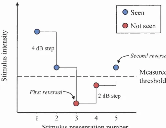
strategy for estimating the sensitivity at a given test location is the 4-2 dB ‘two
reversal staircase’ bracketing strategy (Fig. 1.3). An initial stimulus is presented
whose brightness depends on the results o f tests on nearby points, or on age-
matched normal values. If this is seen, the next presentation at that location is 4 dB
less intense. If this is also seen, the following stimulus at that location is reduced by
a further 4 dB in intensity, and so on until the subject fails to see a stimulus
presentation. This is the ‘first reversal’. The stimuli following this are increased in
intensity by 2 dB each time until the subject again reports a stimulus as seen. This
is the ‘second reversal’. The sensitivity is estimated as the mean of the final and the
penultimate presentation intensities. If the initial presentation is not seen,
intensities of subsequent presentations are increased by 4 dB until one is seen (‘first
reversal’) then decreased by 2 dB until one is missed (‘second reversal’).
O Seen
O Not seen
4 dB step
c
Second reversal
Measured threshold
First reversal
2 dB step
2 3 4 5
1
Stimulus presentation number
1.2.3.2 (ii) Suprathreshold strategies
Pure suprathreshold strategies are simpler and usually faster than full threshold
strategies. Instead of ascribing a numerical estimate of sensitivity to a test location,
they merely record whether it is normal or abnormal. This is done by presenting a
stimulus calculated to be slightly more intense than the patient’s sensitivity
threshold. This calculation requires an estimate of the patient’s threshold: the
various methods by which this is obtained provide the names for the various
suprathreshold strategies. fix e d intensity suprathreshold test assumes that all patients have a similar threshold. Thus the same test intensity is used for all
patients. The age-related suprathreshold test takes account of the fact that
sensitivity declines with age by approximately 1 dB per decade, and uses a table of
normal data along with the patient’s age to calculate the test intensity. The
threshold-related suprathreshold test precedes the suprathreshold test with a determination of the patient’s threshold, usually by means of a brief full threshold
examination using a greatly reduced set of test points. The test intensity is then
calculated relative to this threshold.
The amount by which the stimulus of a suprathreshold test is more intense than the
patient’s threshold, the suprathreshold increment, must be such that a ‘m issed’ point truly represents abnormality (i.e. the stimulus must not be too dim) and a
‘seen’ point truly represents normality (i.e. the stimulus must not be too bright).
M ost perimeters use a suprathreshold increment of between 4 dB and 6 dB. In
addition, most suprathreshold strategies in use compensate for the relatively
reduced sensitivity of the peripheral visual field compared to the central field under
the conditions in which perimetry is performed (lower photopic). These
eccentrically compensated strategies derive an approximation of the hill of vision from their estimates of the patient’s threshold, and thus vary the stimulus intensity
to maintain a constant suprathreshold increment for all test locations.
1.2.3.2 (Hi) Full threshold versus suprathreshold strategies
Full threshold strategies provide more detailed information than suprathreshold
presence or absence. However, full thresholding is more time-consuming, which
has important implications for resource allocation. It is also more wearisome for the
patient, which can affect the reliability of test results. Many patients exhibit
pronounced learning effects: their performance in full threshold testing improves
with repeated attempts (see 1.3.2.2).
For these reasons, suprathreshold testing is best used when a rapid distinction
between normality and abnormality is required, whereas full thresholding is better
for the long-term follow-up of patients whose visual fields are known to be
abnormal and may be slowly deteriorating. For example, suprathreshold testing is
commonly used to ‘screen’ for glaucoma, but patients with established glaucoma
are usually monitored with full threshold tests.
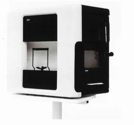
1.2.4 Humphrey Field Analyzer
Data for the studies in this thesis was obtained exclusively from patients tested with
the Humphrey Visual Field Analyzer 630 (Humphrey Instruments Inc., San
Leandro, CA). This machine is described in detail by Haley(^^) and Wemer(^^) and
Figure 1.4 Humphrey Field Analyzer 630 (Humphrey Instruments Inc., San Leandro, CA).
1.2.4.1 Test patterns
The most commonly used testing programs for monitoring the visual fields of
glaucoma patients are the 24-2 and the 30-2, which perform full threshold
estimation (see 1.2.3.2 (i)) at locations within the central 24° and 30° of the field
respectively. The tested locations are 6° apart, with none lying on the horizontal or
vertical meridian. It has been suggested that routine testing at eccentricities beyond
t h i s . T w o nasal locations within the standard 24-2 program lie within this area
out to 30°.
The program which is most frequently used for testing the binocular visual field is
the Esterman Binocular Functional Test. This is a suprathreshold test (see 1.2.3.2
(ii)) which extends to approximately 75° from fixation on the horizontal, 35° above
fixation and 60° below fixation. This test is discussed further in Chapter 5.
1.2.4.2 Graphical display of results
The Humphrey Field Analyzer produces printouts which contain numerical and
graphical data which varies depending on the exact test performed. The most
important features of the printouts are described below.
1.2.4.2 (i) Numerical threshold data
Numbers representing the thresholds measured at all the test locations are displayed
diagrammatically as in Fig. 1.5. The intersection of the two axes represents
fixation, and each number represents the threshold at that test location. For this
particular figure (the Humphrey 24-2 strategy), the separation of the locations, both
15
15 '
ir*
®26
28
à
27
26
17
II)
(i)
25 .28
29
( S )
I)
2 224
2 0(H)
(I)
§1)
" &
27
25
f26
26
2 6
24
24
( I
Figure 1.5 Humphrey Field Analyzer raw sensitivity plot (24-2 strategy)
Numerical displays such as that in Fig. 1.5 may show either the ‘raw’ thresholds at
each location, or they may show the difference in sensitivity between the measured
threshold and a threshold obtained from a normal, age-matched database. For the
Humphrey Field Analyzer, this latter display is called the Total Deviation plot.(^^
The Humphrey Field Analyzer also displays a numerical Pattern Deviation plot:
this is a plot in which any generalised shift away from the age-matched norm is
removed, and only more localised defects are shown.
Although the numerical displays mentioned above provide much useful
information, they are rather dry and difficult to interpret at a glance. The gray scale
provides an image which is more readily understood: thresholds are first
interpolated to give a denser grid of values than the numerical display, then these
are coded according to a key (Fig. \.6b) and displayed as in Fig. \.6a, which is the gray scale corresponding to the numerical display in Fig. 1.5. The Humphrey Field
Analyzer also provides gray scale displays for the Total Deviation(^^) and Pattern
Deviation plots. The appearance of the gray scale is critically dependent on the
method of interpolation used to generate it.(^^)
CRAY SYM flSB DB ■ f. .1
ONE SYMBOLS
1 8
t o
3 . 2 2 5 .
10 32 251
100 794t o
316
2 5 1 2
1000
□
7 ? 4 3 3162 > 10000 50 .3 6 40 .3 1 35 .2 6 30
. 2 1
25
.1 6
20
15. 1 1t o
10
t » 1 <0
Figure 1.6b Humphrey Field Analyzer gray scale legend
1.2.4.2 (Hi) Suprathreshold tests
Since only one of two categories (‘seen’ or ‘not seen’) is attached to each test
location, numerical displays are not appropriate: each location is instead
represented by a symbol indicating whether the stimulus at that location was seen
or not (see Figure 5.1).
1.2.4.3 Global indices
Information relating to the amount of visual field loss, and whether the loss is
generalised or focal, is encapsulated in a set of summary measures known as global
indices. These were first defined for the Octopus perimeter as mean defect, short
term fluctuation, loss variance and corrected loss v a r i a n c e .1 0 1)
corresponding measures for the Humphrey perimeter are mean deviation, short
term fluctuation, pattern standard deviation and corrected pattern standard
deviation.(96) The Octopus indices will be described first as they are more readily
understood and the Humphrey indices are more complex versions of them.
Mean defect is calculated by taking the difference between the threshold measured
at each test location and a value obtained from a normal age-matched database. The
mean defect is the mean of these differences. It is more sensitive to generalised or
diffuse loss than to small, focal scotomas. The validity of the mean defect is
critically dependent upon the validity of the comparison between the test data and
the normal data set. In other words, the sample used to compile the normal database
drawn. This comment applies to all measures which involve a comparison with a
‘normal’ database.
Short-term fluctuation is a measure of the intratest variation. It is calculated by
testing a set of locations more than once during each visual field examination and
analysing the variance of these repeat measures.
Loss variance is an index of the amount of focal loss in the field. It depends on the
fact that, if there are areas of the field with large defects (i.e. differences from
normal values) and other areas with small defects, the variance of the defects will
be larger than if the field were uniformly normal or uniformly depressed.
Since variability is inherent in visual field testing, there will always be some loss
variance. The concept of corrected loss variance was introduced to obtain a zero-
based measure of focal loss. Corrected loss variance is calculated by subtracting
from the value of loss variance a measure of the subject’s intratest variability. This
measure is the square of the short-term fluctuation.
The global indices provided by the Humphrey Field Analyzer have a similar
theoretical basis to the Octopus indices, but there are some important differences.
In the Humphrey Field Analyzer, the formula for the calculation o f a global index
includes a term which accounts for the normal variance at each location. The
Humphrey indices for focal loss, pattern standard deviation and corrected pattern
standard deviation, are related to the Octopus loss variance and corrected loss
variance respectively. However, the Humphrey indices are measures of standard
deviation (square root of variance) as their names suggest, and they incorporate
measures of normal variance at each location as mentioned previously. In addition,
corrected pattern standard deviation includes a constant factor to adjust for the non-
uniform fluctuation pattern across the field. The greater complexity of the
Humphrey indices does not greatly affect their usefulness as summary measures of
visual field behaviour.
The formulae for the Humphrey Field Analyzer global indices are:
where Xi is the measured threshold and Ni is the normal reference threshold at point
i, and s^. the variance of normal field measurements at point i. The number of test
points is denoted by n.(^^)
Pattern standard deviation (PSD)
P S D ^ = |- X s f , } x n —i=l
1 - A ( ; c ,- N ,- M D )
n - l & SÎ,
Short-term fluctuation (SF)
10
1 0-p
S2j XI
10 2 X Sjj
The first and second measured thresholds are denoted by Xj, and respectively.
The normal intra-test variance in point i is denoted by s^j.
Corrected pattern standard deviation (CPSD)
CPSD^ = PSD^ - kxSF^
The constant k (>1) is used to adjust for the non-uniform fluctuation pattem.(^^)
Confidence intervals for normal subjects have been evaluated for all four
i n d i c e s . I f a calculated value falls outside these limits a probability statement is
i 1.2.4.4 The Glaucoma Hemifield Test
The Glaucoma Hemifield test algorithm is provided by the Statpac statistical
program for the Humphrey Field Analyzer. It tests a single visual field for the
presence of a glaucomatous d e f e c t . V i s u a l field test locations are grouped
together in five corresponding pairs of sectors based on the anatomy of the retinal
nerve fibre layer. These sectors are symmetrical about the horizontal midline. Each
sector is compared to its counterpart in the opposite hemifield in order to detect
field loss that is asymmetric about the horizontal meridian. Deviations from the
age-corrected normal threshold in the most sensitive areas of the field are used to
detect overall glaucomatous loss. Fields are classified as outside or within normal
limits, borderline, or as having a general reduction in retinal sensitivity.
1.3 Change in visual field
The detection and quantification of change in visual fields is one o f the most
important and problematic areas of glaucoma management. An early, accurate
measure of whether a field series shows progressive damage is essential: significant
deterioration is likely to prompt a change in treatment, whereas confirmed stability
provides more convincing reassurance than lowered intraocular pressure (TOP)
alone that therapy is successful.
1.3.1 Measurement of change
1.3.1.1 Automated versus manual perimetry
As already mentioned in 1.2.2.2, a benefit of manual perimetry is that an
experienced practitioner can perform fast, flexible testing for a variety o f visual
field abnormalities in subjects who might not be able to produce reliable tests under
the more demanding conditions imposed by an automated perimeter. Manual
open-angle glaucoma estimated from cross-sectional prevalence of visual field
damage in a large, population based study (the Baltimore Eye S u r v e y ) /^^3)
However, for reasons already discussed in 1.2.2.2, the subjective nature of manual
perimetry also limits its effectiveness, since it is a source of variation and bias.
Thus, over the past decade, visual field series consisting of full threshold tests
obtained by automated perimetry have become the standard starting point for
attempts to estimate visual field change in glaucoma.
1.3.1.2 Clinical judgement versus numerical analysis
The most commonly used method of deciding whether a visual field series shows
progression or not is for a clinician to inspect the series visually and use clinical
judgement to form an opinion. Unfortunately, this approach is flawed. Human
observers, even experienced ones, are not able to detect visual field progression
reliably using clinical judgement alone.(1^^) One possible reason for this is that the
standard output of most automated perimeters contains insufficient information
relating to progression or stability. When clinicians are presented with visual field
series which have been processed so as to highlight areas of possible deterioration,
the level of agreement about progression is greater.U05) Thus, although clinical
judgem ent is by definition at the root of clinical decision making, the simple visual
assessment of field series presented as the standard output of an automated
perimeter is an inadequate basis for this judgement. Rather, clinical decisions
concerning visual field progression should be based on the results of computerised
numerical change analysis of visual field series. The most widespread of these
analyses are described below.
1.3.1.3 Summary measures
One group of methods relies on estimates of change in summary measures of the
field such as regression analysis of the mean defect value,(^^) mean deviation,U06)
other global measures,U06) measurement of whole-field and quadrantic sensitivity
losses,(^07) and trend and regression analysis of various estimates of the sensitivity
used to detect incident field loss among patients with elevated intraocular
p r e s s u r e . (109) However, the analysis of summary measures, whether based on the
whole field or on clusters of points within it, has been found to be ‘remarkably
p o o r '(1 1 0) and ‘of little value’(H l) in detecting glaucomatous change. Summary
measures largely or completely ignore the detailed spatial information contained
within computerised field tests and are insensitive to early localised change.(H^)
Furthermore, different regions of the visual field may deteriorate at different
rates. ( 2 1 114)
1.3.1.4 Pointwise measures
Techniques which evaluate progression on a point-by-point basis avoid the
problems with summary measures described above. They may be divided into two
categories: event analyses and trend analyses.
Event analyses rely on detecting a significant change from an established baseline.
For example, the Collaborative Normal Tension Glaucoma Study Group initially
specified an endpoint, based on sensitivity loss, at which patients would be said to
have shown unequivocal deterioration. However, the authors noted a surprisingly
large number of patients reaching the endpoint. Statistical analysis revealed that the
endpoint chosen would be expected to lead to a false diagnosis o f progression 57%
o f the time. In order to correct for this a requirement for progression to be
confirmed on multiple repeat tests was introduced.(^l^) The most recent report
from the Group gives the endpoint as follows: ‘a follow-up visual field was said to
show progression relative to baseline if it contained 2 or more points that had
changed by at least 10 dB relative to the average baseline values for these points;
these 2 progressing points had to be adjacent, both could not be peripheral, both
could not cross the nasal meridian, and the sensitivity at each deteriorating point
had to be less than the minimum of the values of this point in each of the three
baseline visual fields. In addition, progression was also deemed to have taken place
if at least one of the innermost 4 points showed at least a 10 dB deterioration
relative to its average value at baseline, with a value that was less than its minimum
of five consecutive follow-up fields showed progression relative to the baseline
fields, with at least one non-peripheral progressing point (or the one central point)
being common to all four fields.
Trend analyses do not construct a baseline. The behaviour of the visual field is
analysed and progression is diagnosed if a significant tendency to deteriorate is
detected. When this is done on a pointwise basis the technique of linear regression
of sensitivity on time is often used. Test locations are labelled as showing
progression if a significant negative regression line is calculated. For example,
individual test locations from glaucoma patients have been found to deteriorate
significantly at rates of between 1 and 5 dB per year(l®6 117) when visual field
testing is performed annually. The effect of the frequency of visual field testing on
the ability to detect glaucomatous visual field deterioration using pointwise linear
regression is investigated in Chapter 2.
The differences between event analyses and trend analyses may be further
appreciated from a consideration of two commercially available software packages
for the Humphrey Field Analyzer: Statpac 2 (Humphrey Instruments, Inc., San
Leandro, CA, USA) and PROGRESS OR (Institute of Ophthalmology, London,
UK).
L 3 .1 .4 (i) S ta tp a c !
The Statpac 2 Glaucoma Change Probability analysis(H^) performs a pointwise
event analysis. It is the ‘native’ statistical Glaucoma Change Probability software
available as an add-on for the Humphrey Field Analyzer. The program uses the
thresholds from the two most reliable of the first three fields in the series as a
baseline. Each subsequent field is compared on a point-by-point basis to this
baseline. Test locations are labelled with a black triangle (Figure 1.7) if p < 0.05 for
the null hypothesis of no glaucomatous change compared to a database of stable