*Corresponding author: [email protected] 2017 UTHM Publisher. All right reserved. penerbit.uthm.edu.my/ojs/index.php/jst
Automatic Ear Classification System using Lobule Structural Shape
Ugbaga Nkole Ifeanyi
1*, Ghazali Sulong
2, John Isaiah Oluwola
11Computer Science Department, Federal Polytechnic Kaura Namoda Zamfara State, Nigeria. 2Software Department, Faculty of Computing Universiti Teknologi Malaysia.
1. Introduction
Biometrics is a science-based
authentication system which uses physical, behavioural and chemical trait of human being for identification. These characteristics include fingerprint, iris, palmprint, signature, voice, odour, DNA and the ear. The evolution of personal authentication is dated back in the 16th centuries ago, due to proliferation of impersonation cases witnessed that time, and even lead to using pictures of the ear for claimed identity [1]. This necessitated the birth of fingerprint in the early 19th century as biometric character as suggested by Faulds Henry latter of 1880 that the fingerprint patterns are unique and so can be used for human identification. Since then, the use biometrics for various security and criminal confirmation has risen exponentially due to its success for authentication process. Meanwhile, [2] in [3] attempted to identify newborn babies with their ear by studying 206 sets of these ears. They concluded from their experiment that it is possible to distinguish newborn babies from their ears. Furthermore, this have saw major government facilities, building and airport terminals equipped with different biometric scheme to combat crimes like terrorism, information theft, electioneering process and security bridges.
Although some of the biometrics traits such as fingerprint, facial, and iris has since been established to some great extent one would be quick in asking the question why ear
biometric. This is because of its interesting gully shape which remains constant over one’s life span unless in the case of accident. Some of its merit includes, small geometric size, constant colour distribution, and unaffected by emotion or artefact such as creams [4]. Meanwhile, the growing need of security in public places and secluded facilities has made it necessary to use more than one biometric trait for identity authentication; this called multimodal system. For example, a situation where a suspected armed robber covers his faces in a crime scene but left their ear visible in a video surveillance [5]. The ear was later used to uncover the identity of the suspect. Currently, Yahoo is testing an ear-based smart phone identification system [6] whereby smart phone users will start unlocked their phones using ear instead of fingerprint or password. The reason for this new concept is because fingerprint scanners are popular and expensive when compare to smart phone touchscreen.
Earprint analysis has become an active research area since early 20th century during when it was reported that some developed world have started using it as a proof of human identity [7], it is expected that its database will keep multiplying in the course of registering ear for authentication process. This could lead to a huge ear database like that of the fingerprint, and will need some sort of classification to improve. By classifying the ear image will increase computational searching time and accuracy of the ear recognition system. At the same time, would
Abstract: The rate at which ear recognition system is been explored by computer vision authors and its acceptability as a biometric traits has increased. Ear classification scheme has become necessary due to anticipated exponential growth of the ear database which would run to millions in the nearest future. Thus, in this paper, we proposed automatic ear classification scheme so that the ear can be classified into two distinct groups; lobed ear and lobeless ear using geometric structure of lobule. The ear image is cropped and its contrast normalized to produce more quality image. Ear contour image is localized since it can reveal the shape of the ear image. Due to the rumpling nature of the ear, the ear contour harbours many contour images, some which are noisy contours. The ear contour image is enhanced to remove the outer ear contour from the ear contour for feature selection. Using chain code element, ear outer shape is encoded and lobule code signature extracted. Forming a lobule feature code bag, a threshold for the class partition of the ear is established. Experimental result is carried out with University of Science and Technology Beijing (USTB) ear image, which is divided into three samples; 77, 154 and 308 samples respectively. The proposed method achieved an ear classification accuracy of 96.1%, 92.20% and 88.96% under these respective samples.
32
leave out the ears with different class for recognition purpose. Meanwhile, on classifying the ear, it will assist the forensic experts in their forensic examination and analysis. There are various ways in which ear can be classified [8] to reduce searching time by querying ear image in an ear recognition system. They classes is based on the following colour, contour of helix and lobule, anti-helix and anti-tragus, and lobule respectively. Hence an automatic ear classification technique is proposed in this paper. With this technique, a recognition system needs not to query the entire database rather a partition which matches with the querying ear image. This paper is organized as thus; section 2 – briefly discusses the anatomy of the ear and in section 3 – pre-processing. Section 4 – feature extraction, while section 5 - experimental result. And finally section 6 – conclusion.
2. Ear Anatomy
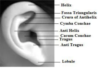
Human ear is a special organ located at both sides of the face which is used for hearing. The ear is made up different parts; outer (Pinna), middle and the inner ear. For the purpose of building a recognition system the Pinna, which the visible part of human ear is used for access authentication process. The ear is viewed the as a small hearing organ with a multipart which also aids human balance [9]. This multipart make up the huge gullies which serve as a pattern for recognition process and the parts includes; the Helix, Fossa Triangularis, Crura of Antihelix, Cymba Conchae, Anti Helix, Cacum Conchae, Tragus, Anti Tragus and Lobule. Fig. 1 depicts the outer ear (Pinna) with its different parts.
Fig. 1 Ear anatomy.
Though the outer ear (Pinna) shape is by nature made to assist in directing sound into the middle and inner ear, biometric basically uses it for identification because of its unique structure either in crime scenario or access
authentification purposes. Ear recognition system has become a major focus in the biometrics world because of its interesting gully shape which remains constant over one’s life span unless in the case of accident [7], [10], [11], [12], [13], [14]. Ear image can be captured with different devices such as CCD camera, mobile phone, cameras and other devices which can serve the purpose; and are stored in a database for future use. The visual cognition human experts on human ear can be linked on the structural representation of the ear. This structural shape makes ear so unique that no two ear have the same shape, even ones from same individual [15], [7], [16], [3], [17], [18], [19], [20], [21], [22]. Hence, the ear can be professionally grouped into two physiological classes based on the lobule structure. And to equip the system with human expert knowledge based on lobule classes before recognition system, this paper made used the lobule.
3. Ear Pre-Processing
After the acquisition of ear image with a digital device, the resolution and lightening condition of the scenario might cause variation in the acquired image. Variations in image qualities due to environmental condition and pose angle, mostly contributes to the variation found in the same images captured at different time [23]. Pre-processing is done to ensure that images are prepared for examination and interpretation [24]. Meanwhile, [25] submitted that image pre-processing involves numerous operations like brightness, contrast, and geometric distortion correction. Thus, for an efficient system, pre-processing becomes inevitable to ensure a quality ear image going further of processing. The pre-processing activities performed here include; ear cropping, contrast enhancement, orientation normalization, ear contour localization, and enhancement respectively.
3.1 Ear Cropping
33
filter for smoothing, Sober filter for tracing gradients, non-maximum suppression, thresholding and hysteresis. This process makes it more efficient in contour detection when compared to other operators with respect to the problem under review. Fig. 2 depicts the output of the process which is presented for cropping activity.
Fig. 2 Detected ear edge image
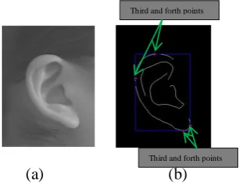
The second step continued with the exposed boundary edge of ear image. The binarised ear image consists of white ‘1’ and black ‘0’ pixels. This edge image is scanned from row-wise from top left to right and column-wise from top left to bottom locating the first white pixels in each case. This process is repeated, but this time from bottom right to left and bottom right to top also locating the first white pixels. This two set of processes is performed to locate the coordinates of the bounding box which is used for cropping. The image is then cropped with a ten pixel distance allowance from the detected points in other to ensure that the ear image is within the image frame. Fig. 3 show the four basic points that is used in constructing the bounded box for cropping.
Fig. 3 Point Localization. (a) Original image. (b) Edge Image and its bounding box
The ear image is cropped by allowing ten number of pixel distances from the detected image boundary depending on the image, to ensure that the image itself is not compromised during cropping. The Fig. 4
shows the cropped image from the original image and this reveals that some unwanted information that might have gone into process.
Fig. 4 Image Cropping. (a) Original ear image with bounded box
(b) Cropped ear image
3.2 Ear Contrast Normalization
Image contrast normalization is a process used to improve the quality of ear image by altering the pixel intensity value to a particular range of values. Usually, any image processing systems always have the problem of contrast to deal with. This problem most times originates from either the camera or the environmental condition under which the image was taken. Having cropped the ear image as highlighted previously, the image is enhanced to improve the image contrast variations which will assist in ear contour detection. This is done to ensure an equal distribution of brightness in the image, since some of the images from the database have no much variation in areas in the image. In doing so, those pixels whose values are above or below a specific value are represented as either white or black, while those within the range is set to gray respectively. This is implemented using Eq. 1 and Eq. 2. Fig. 5 depicts the grayscale value distribution before and after.
PRange = V(i) – U(i) (1)
N_Img =255 ∗ I(x, y) − U(i) PRange
(2)
Where
PRange: Pixel range value V(i) : Maximum pixel value
U(i) : Minimum pixel value
I(x, y): Original image
N_Img: Normalized image
(a) (b)
Third and forth points Third and forth points
34 Fig. 5 (a) Original ear image (b) Histogram
of original image (c) Normalized ear image (d) Histogram of normalized image
3.3 Ear Image Orientation Normalization
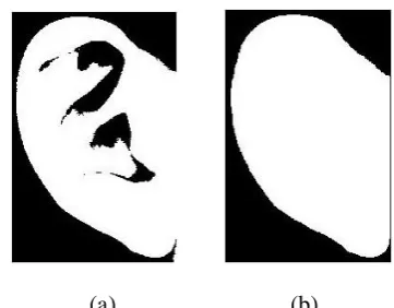
After a successful contrast normalization process, the ear image is then normalized in terms of orientation using the ear image landmark. This is achieved by aligning then to a reference point for the purpose of harmonizing the point of origin for the whole images in the database and extraction of features at the same area for all the images. Ear landmark point is the salient area which is same in their localization that is used for proper alignment of ear image. The normalization is achieved by binarizing the ear image so that we have black background and white foreground and because of the uneven distribution of the pixels intensity values in the image, some holes might be present within the foreground as in Fig. 6(a).
Fig. 6 (a) Binarised ear with holes on the foreground (b) Enhanced binarised ear
To remove these black pixels on the foreground, morphological opening is applied to produce an enhanced image as in Figure 6(b). This is used to remove the black pixels over the foreground. The enhanced binarised image is now scanned pixel by pixel starting from the top left corner to the right to locate the first and last white pixel along the row at helix and lobule of the ear image as shown in Fig. 7(a). A landmark line is constructed using the two localized points as in Fig. 7(b). Having located the ear image landmark, the angle of rotation is calculated. This is achieved by constructing a triangle using the image landmark line as shown in Fig. 7(c). The orthogonal and horizontal distances are computed using the Eq. 3 and Eq. 4. The angle of rotation A, as marked in the figure can calculated using the Eq. 5 and Eq. 6.
(a) (b)
(c) (d)
(a) (b)
35 Fig. 7 (a) Detected landmark points
(b) Constructed landmark line (c) Estimated angle of rotation (d) Rotation ear image
x = √(x2− x1)2+ (y2− y1)2 (3)
y = √(x3− x2)2+ (y3− y2)2 (4)
Angle = atan (y
x) (5)
Rotangle = Angle − 90 (6)
Where
x : is the horizontal and y : vertical axis,
𝑥1, 𝑥2, 𝑥3 𝑎𝑛𝑑 𝑦1, 𝑦2, 𝑦3are pixel co-ordinates
Angle : angle between the landmark and
horizontal axis
Rotangle
: computed angle of rotation.
The ear image rotation is the transformation of the image by positioning it into a similar planar space. Ear image is then rotated using the estimated rotational angle so that they are aligned as shown in Fig. 7(d).
3.4 Ear Image Contour Detection and Enhancement
After the ear image has been normalized in terms of orientation, the contour of the ear is localized. This is achieved by using canny edge operator because it consists of different processes toward getting the contour image. Thus, this process makes it more efficient since it leaves a single length pixel contour which is required by this research as shown in Fig. 8
Fig. 8 (a) Detected ear outer edge image (b) Enhanced outer contour
After contour detection, many contours are revealed because of the rumpled structure of the ear as in Fig. 8(a). The contour enhancement is performed to remove contours produced by the ear internal structure to recover the outer ear shape, which is required for further processing. This is achieved by scanning the contour image using 8-connected neighbourhood to locate and remove the frame and internal contour which constitutes noise in this case. Fig. 8(b) shows the enhanced ear contour image with only the outer contour ear image.
4. Ear Image Feature Extraction
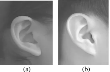
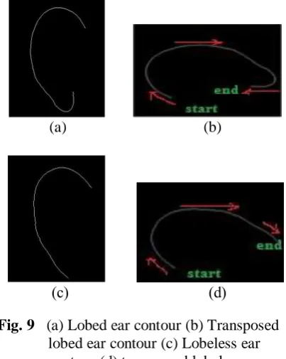
The process involves two major steps, they includes: translation of outer ear contour image and pixel orientation extraction. Because of proven spatial structure descriptor prowess, chain code would perfectively preserve lobule structure of the human ear used for classification in this research. For those reasons, this research proposed the classification of human ear image using lobule chain code. This is inspired by the structural shape of the lobule, taking a leaf from the professional points of view. The ear is grouped into two classes; lobed or lobeless, while the former has the ear lobule attached to the head, in the latter lobule is seen unattached to the human head, this is depicted as in Fig. 9.
Fig. 9 (a) Lobed ear (b) Lobeless ear
(c) (d)
(a) (b)
36
For the purpose of encoding the outer ear contour image using the chain code, the starting point needs to be localized. This is achieved by transposing the ear outer contour image as shown in Fig. 9(a, c) and Fig. 9(b, d). The contour image is transposed so that a unique starting point for the chain code is established. The transposing process is done by looping through the image making all the rows to columns and columns to rows. The chain code of the ear contour is extracted by starting from the first pixel point of the contour when scanning from the bottom left to right of the binary image.
Fig. 9 (a) Lobed ear contour (b) Transposed lobed ear contour (c) Lobeless ear contour (d) transposed lobeless ear contour
There are two basic connectivity principles for encoding the contour and boundaries using chain code [16], they include 4-neighbours connectivity and 8-neighbours connectivity as depicted in Fig. 10. The 8-neighbours connectivity was used in this paper because it moves in all four cardinal directions and the diagonals making it possible to trace all the contour orientation movement in a raster representation. Meanwhile, the encoding process follows a clockwise movement from the starting point, moving through the contour pixel by pixel storing the orientation of the unit pixel width of the contour which is spatially connected using 8-connected neighbourhood. This movement is repeated
until the last pixel in the contour is encountered.
Fig. 10 (a) 4-neighbour connectivity (b) 8- Neighbour connectivity
4.1 Design of Ear Image Classification
The extracted code sequence above represents the ear structural shape from ear outer contour image. In order to group the ear image into two established classes (lobed and lobeless) using the extracted code signature, the part representing the lobule of the ear shape have to be localized. This process requires three key stages: (1) Understanding the structure of lobule, (2) Establishing the number of code sequence that can represent the lobule shape and (3) Extraction of lobule-feature code bag. The first stage involves two phases: (i) Examining the unique code at lobule (ii) Determine the frequency of occurrences of the unique code. To achieve this, the entire code signatures from different ear outer contour image were empirically examined, and it was observed that code 7 element could play a discriminating factor among the two groups. Having confirmed the uniqueness of code 7 element for the representation of the two ear groups, its occurrence on each of the groups was also determined. Meanwhile, the other step was ascertained by experimental examination. It is established that from experiment perform code 7 element outperformed code elements 5 and 6 respectively. At the same time, four different numbers of code sequence set were examined, they includes 10, 15, 20, 30, and 45 respectively, to establish the length which truly represent the lobule in this system. It was revealed that, 15 numbers of code sequence efficiently describes the lobule structure amongst others.
(a) (b)
(c) (d)
37 4.2 Design of Ear Image Classification
The extracted chain code from the ear contour is a sequence of numbers from (0-7), representing the structure of the entire ear image. It is pertinent to note that, the proposed grouping technique used the code signature of the lobule since the scheme is lobule-based. That is, only the structural shape of the lobules is significant for the proposed ear grouping. This lobule code signature is situated toward the end portion of the extracted ear code. Using only the lobule code instead of the entire chain code drastically minimises chain code side effect and increases the accuracy of the classification technique. Since emphasis is now focused on the ear lobule part only. To extract the lobule code, the entire code sequence is stored in the reverse order so that the last code signature becomes the first and the first the last. The flowchart of this ear classification technique is shown in Fig. 11.
Fig. 11 Ear classification flowchart
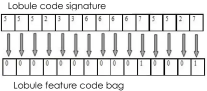
The first fifteen code element was empirically selected to represent the lobule code signature. In order to partition the ear into two classes: lobed and lobeless, a thresholding value between then is to be established. This is achieved by feature selection process designed as follows: from the lobule code signature which is now fifteen code length. If code element from 0 to 6 is found in the lobule code signature, a zero is assigned to feature bag and if code 7 element, a 1 is assigned to the feature bag as in Fig. 12.
Fig. 12 Feature extraction using Lobule signature
Thus, this feature bag called lobule-feature code bag is designed. Since it contain lobule code for each ear contour image, and it is now made up of values 0’s and 1’s. Having earlier ascertained that lobeless ear image has a minimum of seven occurrence of code 7 element in the lobule-feature code bag, this minimum number seven is used to divide the length of lobule code which is fifteen, to determine the threshold value for class distinction. Hence, the threshold, T = 15 7⁄ = 2.14 for the class partitioning of the two ear types based on lobule shape.
5. Experimental Results
To evaluate the ear classification method performance, three different sets of experiment was carried out with different numbers of samples from database which includes; the first set used all the 308 images in the database as coming from different subjects, while the second set uses 154 image which were ears images captured under standard and weak illumination, and the last set used 77 ear image captured under standard environment. To calculate the error rate, the formular in Eq. 6, this is the percentage of misclassified ear to total number of ear sample used in the experiment. The accuracy of the system can be computed using formular in Eq. 7.
Lobule code signature
38 𝐸𝑟𝑟𝑜𝑟 𝑅𝑎𝑡𝑒 (𝐸𝑅) = 𝑇𝑜𝑡𝑎𝑙 𝑛𝑜 𝑜𝑓 𝑀𝑖𝑠𝑐𝑙𝑎𝑠𝑠𝑖𝑓𝑖𝑒𝑑 𝑒𝑎𝑟
𝑇𝑜𝑡𝑎𝑙 𝑛𝑢𝑚𝑏𝑒𝑟 𝑜𝑓 𝑒𝑎𝑟 𝑖𝑚𝑎𝑔𝑒 × 100% (6)
𝐴𝑐𝑐𝑢𝑟𝑎𝑐𝑦 𝑅𝑎𝑡𝑒 (𝐴𝑅) = 100% − 𝐸𝑟𝑟𝑜𝑟 𝑅𝑎𝑡𝑒 (7)
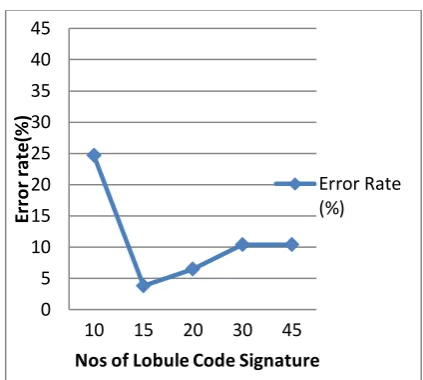
The performance of the classification scheme starts with evaluation of lobule code signature length using the ear captured under standard environment which contains 77 ear images. That is an appraisal of the length of chain code which will effectively represent the lobule shape as discussed earlier. This is achieved by varying the length of lobule in the following order 10, 15, 20, 30 and 45 as depicted by Table 1 with the use of the metric in Eq. 5 and 6 respectively. The table summarizes the performance of lobule code signature length, suggesting the best length that can represent the lobule shape image is 15, while length of 10 has the lowest accuracy rate.
Table 1 Performance of the proposed classification technique with regard to code number.
The results were pictorially explained using the graph in Fig. 13, which shows an exponential fall in the error rate from 24.5% to 3.8%. This can be attributed to the increase in range which for which the code 7 element occurrence can be counted. Because, the higher error rate at 10 did not accommodate much of the lobeless ear since that is now represented in 15. Moving further to code length of 20, it can be seen that error rate started increasing again. This is because some of lobed ear image have an increase in the number of code 7 element, resulting to them being misclassified as lobeless ear. In the same vein, the error rate increased with a difference of 4.2% for length 30. As the length of code signature was increase to 45, the error rate remains constant at a length code signature of thirty. Any further increase in length does not have any effect on the error rate.
Fig. 13 Error rate as a function of number of code pattern.
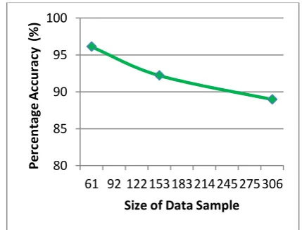
This is showed on the graph by a sharp decrease in the error rate due to better representation of both ear classes at for length fifteen, but immediately started rising again until it became constant. With this result, it is established that the minimum error rate the new method can achieve under different length code signature is 3.8% with fifteen lobule code signature length, thus, any length below or above is size will be compromising the accuracy of the system. Furthermore, the experimental performance of the two other data samples showed a fall in the accuracy rate as shown in Table 2. It can be seen that the performance of database with highest subject recorded the lowest accuracy rate, this can be attributed to the increase of noisy ear image which made the system not to even register the ear image much less of grouping it.
Table 1 Comparison of classification scheme as a function of USTB data sample
S/No Size of
sample
Accuracy rate (%)
1. 77 96.10
2. 154 92.20
3. 308 88.96
The performance evaluation of the first sample to the second shows a 3.9% decrease in accuracy rate which signifies that only that percentage of ear image were misclassified or was not even able to capture by the system due to noise. Meanwhile, the accuracy of the process decreased in the third sample, with 7.1% error rate difference with the first and
0 5 10 15 20 25 30 35 40 45
10 15 20 30 45
Err
o
r
ra
te
(%
)
Nos of Lobule Code Signature
Error Rate (%)
Lobule code signature
10 15 20 30 45
Error Rate (%)
39
3.24% with the second. The performance
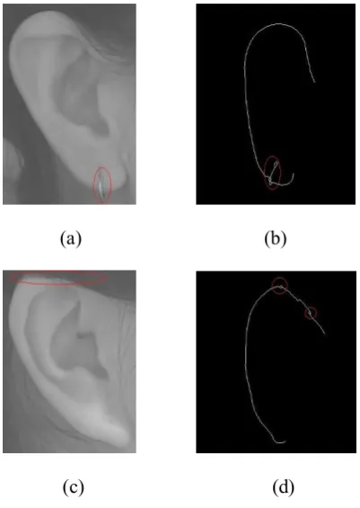
accuracy of the proposed method failed during registration process due to the following reasons: Firstly, there were no much contrast variations between the skin beneath the ear and the extended helix part in some of the ear image. The non variation of contrast is as in the circled areas in Fig. 14(a) was the reason for ear contour image distortion as depicted in Fig. 14(b). Secondly, some of the artefact (hair, earring and spectacle handles) as depicted in Fig. 14(c), presented a false ear contours as in Fig. 14(d), thereby altering its natural structure. With such distortions, the single outer ear contour image for the scheme cannot be extracted as required. Lastly, protruding ear structure in Fig. 14(e) produces poor view from angle of acquisition, thus, creating irregular ear contour away from normal ear structure which is described in Fig. 14(f). Some of these ear image samples are as attached in Appendix.
Fig. 14 Noisy ear image and their associated noisy contours
The performance of the system decreases as the number of samples increases because as depict in Fig. 15, this is due to number of images that failed to be registered. The first samples are images captured under normal condition while the second and third were an inclusion of the images captured under environmental influence. These results are very encouraging as it is expected that if operators could get high level of co-operation from the subjects during ear image acquisition stage; the proposed ear classification scheme could perform better.
Fig. 15 Comparison of database size as a function of percentage accuracy
However, it is observed that in some cases where there is occlusion either at the helix or lobule with a single contour flow without interference on the structure of outer ear contour structure movement, a perfect classification process is achievable. This is because the chain code can be able to trace the shape of the contour without any branching as depicted in Fig. 16(a), owning to the fact that the lobule structure is still preserved though with a distorted helix. Similarly, in Fig. 16(b), where the earring is hosted by the lobule, although with disturbed lobule contour, the classification scheme is expected to also group the ear image correctly. This is because the false contour created by the earring did not really distort the area used as lobule shape structure for the classification.
80 85 90 95 100
61 92 122153183214245275306
P
e
rc
en
ta
ge
A
cc
u
ra
cy
(%
)
Size of Data Sample
(a) (b)
(c) (d)
40 Fig. 16 (a and c) Noisy ear image
(b and d) Noisy helix and lobule
5. Conclusion
We have proposed a new automatic ear classification system based on lobule structural shape. Ear image is cropped from right profile face image before contrast was normalized on the image. The ear contour image is then localized and enhanced to extract the outer ear contour. Extracting the pixel orientation of the ear, the lobule code signature was selected. This code signature was used to design a lobule feature bag that was used for classification of ear image into lobed and lobeless. It is expected that this technique would reduce the searching time of any ear recognition system since it will now be concentrated on a subset of the database instead of the whole database. At the same time assist forensic analysis expert in their course of criminal investigations.
References
[1] Hurley, D. J. (2001). Force Field Feature Extraction for Ear Biometrics. Doctor of Philosophy Thesis, University of Southampton, Southampton.
[2] Fields, C., Hugh, C. F., Warren, C. P. and. Zimberoff, M. (1960). The Ear of the Newborn as an Identification Constant. J. Obsts. Gynae., 16: 98-101.
[3] Purkait, R. (2007). Ear Bimetric: An Aid to Personal Identification. Anthropology Today: Trend, Scope and Application, Anthropology Special Volume, 3: 215-218
[4] Xiu-qing, W., Hong-yang, X. and Zhong-li. W. (2010). The Research of Ear Identification Based On Improved Algorithm of Moment Invariant. Information and Computing International Conference (ICIC), 2010. Wuxi, Jiang SU, China. 4-6 June 2010. 58-6
[5] Ross, A., and Abaza, A. (2011). Human Ear Recognition. IEEE Computer Society, 44(11): 79-81.
[6] British Broadcasting Corporation New.
(2015). Technology. From:
http://www.bbc.com/news/technology-32498222.
[7] Choraś, M. (2004). Ear Biometrics Based on Geometrical Method of Feature Extraction, in Articulated Motion and Deformable Objects. Springer Berlin Heidelberg, 51-61.
[8] Ross A. (2011). Advances in Ear Biometrics. A presentation, From: 2012.Url:http:// www. biometrics .org/bc2011/presentations/FaceTechnolo gy/0928_1600_Mr15_Ross.pdf
[9] Irwin, J. (2006). Basic Anatomy and Physiology of the Ear. Infection and Hearing Impariment. John Wiley and
Sons, Ltd.
From:http://media.johnwiley.com.au/pro duct
_data/excerpt/70/18615650/1861565070. pdf
[10] Yan, P. and K. W. Bowyer. (2005). Empirical Evaluation of Advanced Ear Biometrics. Proceeding of the 2005 IEEE Computer Society Conference on
Computer Vision and Pattern
Recognition (CVPR'05).San Diego, CA, USA.
[11] Arbab-Zavar, B., Nixon, M. S. and Hurley, D., J. (2007). On Model-Based Analysis of Ear Biometrics. First IEEE International Conference on Biometrics:
Theory, Applications, and
Systems,(BTAS) 2007. Crystal City, VA. 27-29 Sept. 2007. 1-5.
[12] Heng, L. and Dekai, L. (2010). Improving Adaboost Ear Detection with Skin-color Model and Multi-template Matching. Computer Science and
(a) (b)
41
Information Technology (ICCSIT), 2010 3rd IEEE International Conference. Chengdu. 9-11 July 2010. 106-109. [13] Tahmasebi, A., Pourghassem, H. and
Mahdavi-Nasab, H. (2011). An Ear Identification System Using Local-Gabor Features and KNN Classifier. Machine Vision and Image Processing (MVIP), 2011 ,IEEE. Tehran, Iran. 16-17 Nov. 2011. 1-4.
[14] Rathore, R., Prakash, S., and Gupta, P. (2013). Efficient Human Recognition System using Ear and Profile Face. Biometrics: Theory, Application and Systems (BTAS), 2013 IEEE sixth International Conference. Arlington, VA. Sept. 29 – 2 Oct. 2013. 1-6.
[15] Burge, M., and Burger W. (2000). Ear biometrics in computer vision. 15th International Conference in Pattern Recognition, 2000. Proceedings.
[16] Jain, A. K., Ross, A., and Prabhakar, S. (2004). An Introduction to Biometric Recognition. IEEE Transactions on Circuits and Systems for Video Technology. 14(1). pp. 4-20, January 2004.
[17] Zhang, H., and Mu, Z. (2008). Compound Structure Classifier System for Ear Recognition. IEEE International Conference in Automation and Logistics. pp. 2306-2309, September 2008.
[18] He-lei, W., Qian, W., Hua-jun, S., and Ling-yan, H. (2009). Ear Identification Based on KICA and SVM. Intelligent Systems, 2009. GCIS '09. WRI Global Congress.Vol4. pp. 414-417, May 2009. [19] Alaraj, M., Hou, J., and Fukami, T.
(2010). A Neural Network Based Human Identification Framework using Ear. TENCON 2010-2010 IEEE Region 10 Conference. pp. 1595-1600, November 2010.
[20] Chan T.-S., and Kumar A. (2011). Reliable Ear Identification using 2-D Quadrature Filters. Pattern Recognition Letters, 2011. pp. 1-26.
[21] Kumar, A., and Wu, C. (2012). Automated Human Identification using Ear Imaging. Pattern Recognition, Future Information Technology (FutureTech), 2010 5th International, 45(3). pp. 956-968, March 2012.
[22] Rahman, M., Sadi, M. S., and Islam, M. R. (2014). Human ear recognition using
geometric features. Proceedings of the 2014 Electrical Information and Communication Technology (EICT), 2013 International Conference on, pp.13-15 Feb. 2014. pp. 1-4.
[23] Adini, Y., Y. Moses and Ullman, S. (1997). Face recognition: the problem of compensating for changes in illumination direction. IEEE Transactions on Pattern Analysis and Machine Intelligence, 19(7): 721-732.
[24] Russ, C. John. (2007). The Image Processing Handbook. 5th Edition, Taylor and Francis Group, Boca Raton USA.