Weather Generator Application with Mixed Exponential
Distribution Representing Rainfall Intensity
Syafrina, A. H.∗1, Noor Shazwani, O.2, and Norzaida, A.3
1Department of Mathematics, Faculty of Science, Universiti Putra Malaysia, UPM
Serdang, Selangor, Malaysia
2UTM Razak School of Engineering and Advanced Technology, Universiti Teknologi
Malaysia, Kuala Lumpur, Malaysia
3UTM Razak School of Engineering and Advanced Technology, Universiti Teknologi
Malaysia, Kuala Lumpur, Malaysia
∗Corresponding author: [email protected]
Adequate and accurate rainfall information is vital in hydrological forecasting, however historical data are sometimes inadequate or nonexistence at location of interest. Stochastic weather generator which is developed based on historical metrological data, is often employed to generate synthetic rainfall series. In this study, the Advanced Weather Generator or AWE-GEN is employed to generate hourly rainfall series in the state of Johor, Malaysia. Within the AWE-GEN, is the Neyman Scott model to assess rainfall series. This study proposed the use of Mixed Exponential distribution in representing rainfall intensity of the Neyman Scott model. AWE-GEN is developed based on meteorological data from period 1975-2015. The model is then used to generate rainfall series separately at two sites within Johor. Generated results were found to be comparable to the historical rainfall series at both sites. Although rainfall distribution at the two sites are influenced by different monsoon winds, the model is able to capture significant statistical characteristics of rainfall behavior at each site. The successful development of this model could be beneficial in addressing issues such as insufficiency of rainfall data at rainfall stations. In addition the model could be employed to generate data as input to various hydrological models.
Keywords: stochastic model, metrological data, rainfall intensity, probability distribution, weather generator.
I.
Introduction
Stochastic weather generator is a statistical model of observed weather variables, with vari-ables generally conditioned on the occurrence of precipitation (Fowler et al. (2007), Hashmi et al. (2011)). Such models provide the means to downscale large-scale climate data at both spatial and temporal scales. Over the years, various weather generators have been devel-oped and improvised in order to produce re-liable output, for example the Weather Gener-ator (WGEN) (Richardson (1981), Richardson and Wright (1984)), Climate Generator (CLI-GEN) (Nicks et al. (1995)) and Long Ashton
underestimate monthly and inter-annual vari-ances due to lack of consideration in estimating the low-frequency component of climate vari-ability (Kilsby et al. (2007)). Dubrovsk`y et al. (2004) used a monthly generator (based on first-order autoregressive model) to adjust the low frequency capability based on daily WGEN model. Despite the well simulated results, this model could not capture the inter-annual vari-ability. Wang and Nathan (2007) has intro-duced the method for the pairing of two differ-ent time scales modeled stochastic hydrological time series model. Two resembling time series were produced, one preserves important statis-tical properties on a finer time scale and an-other one is on a coarser scale of time. The ad-justment is made on a series of finer time scales so that the series is consistent with a series of coarser time scales. The results show that the coupling method is able to produce a series of daily rainy days which preserves some im-portant statistical properties on daily, monthly and yearly scales. Other studies of weather generator (Chen et al. (2011), Furrer and Katz (2008), Keller (2015), Semenov (2008), Wilby et al. (2002)) were also conducted to address problems related to daily weather generator. In addition, Mehan et al. (2017) have compared the performance of different stochastic weather generators for long term climate data simula-tion. In particular, CLImate GENerator (CLI-GEN), Long Ashton Research Station Weather Generator (LARS-WG), and Weather Genera-tors (WeaGETS) were compared in terms of their ability in capturing important statistic features. The observed daily monitoring sta-tistical features and minimum and maximum daily air temperature were well simulated using both CLIGEN and LARS-WG models. These generators can also simulate maximum growth periods and increasing degree days, making them ideal for plant growth simulation. How-ever, WeaGETS model is not quite well in cap-turing the descriptive statistics, output value distributions, and evaluation of extreme vari-ables. Recent study by Keller et al. (2017) has applied the weather generator for climate
downscaling approach over Switzerland. The multi-variate weather generator has been used to downscale future daily weather time-series (precipitation, minimum and maximum tem-perature). The weather generator was cali-brated at the individual stations over a refer-ence period of 30 years (1980–2009) and run under future climate conditions for the A1B Special Report on Emissions Scenarios (SRES) scenario period from 2070 to 2099.
In Malaysia, Hassan and Harun (2013) has applied LARS-WG model to downscale the fu-ture daily rainfall at the catchment Kerian in Perak state. Results indicated that daily rain-fall was projected to be decreased under A2 SRES scenario. The performance of LARS-WG has also been compared with Statisti-cal DownsStatisti-caling Model (SDSM) (Hassan et al. (2014)). It was found that SDSM yields a bet-ter results compared to LARS-WG, although SDSM slightly underestimated the wet and dry spell lengths. Both models indicate a general increasing trend in the mean daily tempera-ture values (Hassan et al. (2014)). Similarly, an AWE-GEN (Advanced Weather Genera-tor) model, developed by Fatichi et al. (2011), has been applied over Peninsular Malaysia to reproduce a broad range of temporal scales in weather variables from the high-frequency hourly values to the low-frequency inter-annual variability. However, in contrast with the ear-lier study, this weather generator had projected an increase in extreme rainfall events under Representative Concentration Pathway (RCP) 6.0 scenario (Syafrina et al. (2018)). The re-sults are consistent with Pachauri et al. (2014) in which the studies indicate a positive trend of rainfall over the Malaysia region between 2001 and 2099.
to be the best distribution of rainfall inten-sity in Peninsular Malaysia to model the rain-fall intensity (Hassan et al. (2015)). Another study found that Mixed Lognormal distribu-tion was the best distribudistribu-tion model for most of the rain gauge stations in Peninsular Malaysia (Suhaila et al. (2011)). Studies by Abas et al. (2014) and Daud et al. (2016) using Neyman Scott methodology showed that Mixed Expo-nential was the best distribution to describe the intensity of rainfall in Peninsular Malaysia. Based on the successful use of Mixed Expo-nential distribution in Malaysia, the main aim of this study is to evaluate the capability of the said distribution in a weather generator, namely AWE-GEN. Since finer resolution rain-fall data has many uses in extreme event stud-ies, the study focuses on data at hourly scale. The study site is situated in Johor, Malaysia where the occurrence of flooding is quite fre-quent. In this paper, the data involved are de-scribed in Section 2 while methodology used is in Section 3. Next, the results are discussed in Section 4 and lastly, the conclusion is presented in Section 5.
II.
Methodology
Located near the equator, Malaysia experiences a tropical climate with high temperatures and rain all year long. Monsoonal rainfall is becom-ing more erratic and unpredictable from year to year (Lim and Samah (2004)). Malaysia experiences two monsoon seasons; the south-west monsoon between mid to October and the northeast monsoon from October to March. The east coast of Peninsular Malaysia con-tinues to be affected by the northeast mon-soon which brings higher rainfall amount than southwest monsoon. The focus area in this study, Johor is situated in the southeastern part of Peninsular Malaysia and is located be-tween the 1o20’N and 2o35’N latitudes. Johor has total land area of 19,210 km2 and a popu-lation of about 3.2 million as of 2010. Johor’s rainfall distribution is governed by southwest monsoon (November to February) which brings
heavy rain, resulting in frequent flooding occur-rences during this period. The average annual rainfall is 2355 mm with average temperature ranging between 25.5oC and 27.8oC.
In this study, the AWE-GEN model is con-structed based on 41 years of historical data (1975-2015). The input data required by AWE-GEN are hourly scaled data such as rain-fall, temperature, relative humidity and wind speed. Rainfall data were sourced from the Malaysia Drainage and Irrigation Department (DID) while the other meteorological data were sourced from Malaysian Meteorological De-partment (MMD).
In AWE-GEN model, the proposed Mixed Exponential distribution is fitted to the inten-sity of rainfall and the intra-annual variabil-ity of rainfall is captured by the Neyman-Scott Rectangular Pulses (NSRP) model. Work by Abas et al. (2014) and Norzaida et al. (2016) indicated that the NSRP model is suitable to be used in Malaysia. The proposed model is then used to generate hourly rainfall series sep-arately at two stations within the state of Jo-hor. Simulated results are then compared with the observed data. Figure 1 shows the location of the rainfall stations whereas Table 1 lists the selected stations used in this study. The Mixed Exponential distribution that is associ-ated with NSRP is as in Equation (1) where
ξ (light rain) and θ (heavy rain) are the scale parameters,αis the mixing probability param-eter; set to a constant, 0.65 following Fadhi-lah et al. (2008) and x is the hourly rainfall amount. Table 2 gives the definition of each rainfall parameter estimated by NSRP model.
f(x) = (α/ξ)e−x/ξ+ ((1−α)/θ)−x/θ (1)
forx >0, 06α61, 0< ξ < θ
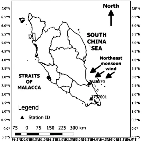
Figure 1: Location of rainfall stations
Table 1: Name of stations with station ID, latitude (Lat) and longitude (Lon)
Station ID Name of Station Lat(oC) Lon(oC)
1737001 Sek. Men. Bukit Besar, Kota Tinggi Johor 1.76 103.74
2636170 Stor JPS Endau, Johor 2.65 103.62
Table 2: Rainfall parameters of the NSRP model.
Parameter Definition
λ Mean storm origin arrivals (h)
β Mean waiting time for cell origins after the origin of the storm (h)
η Mean duration of the cell (h)
µc Mean number of cell per storm [-]
α Mixing probability
ξ Scale parameter (light rain)
θ Scale parameter (heavy rain)
the reference period where the multiplicative factor is calculated based on the simulation output and the high resolution observational data. The changing factors will then be used to correct the biases of the simulation output from 1996 to 2015. The revised hourly rain-fall is then compared to the observation from the identical period of 1975 to 1995. Genera-tions of rainfall series with respect to extreme rainfall and dry/wet spell lengths at each
rain-fall station are conducted using the identified distribution.
III.
Results and Discussion
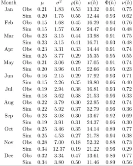
pe-Table 3: Statistical properties at 1-hour aggregation period for Station 1737001.
Month µ σ2 ρ(h) κ(h) Φ(h) ν(h)
Jan Obs 0.21 1.83 0.53 13.32 0.91 0.75
Sim 0.20 1.75 0.55 12.44 0.93 0.62
Feb Obs 0.15 1.68 0.45 16.29 0.94 0.76
Sim 0.15 1.57 0.50 24.47 0.94 0.48
Mar Obs 0.23 3.15 0.44 13.98 0.91 0.75
Sim 0.23 3.15 0.41 16.71 0.93 0.48
Apr Obs 0.23 3.31 0.33 14.44 0.91 0.74
Sim 0.25 3.77 0.29 15.35 0.95 0.55
May Obs 0.21 3.06 0.29 17.05 0.91 0.74
Sim 0.20 3.96 0.15 22.66 0.95 0.23
Jun Obs 0.16 2.15 0.29 17.92 0.93 0.71
Sim 0.15 2.26 0.35 19.80 0.96 0.40
Jul Obs 0.19 2.94 0.38 16.81 0.93 0.72
Sim 0.18 3.62 0.38 21.53 0.96 0.33
Aug Obs 0.22 3.79 0.30 22.95 0.92 0.74
Sim 0.22 5.92 0.37 32.79 0.96 0.36
Sep Obs 0.23 3.08 0.30 13.67 0.92 0.69
Sim 0.19 3.91 0.31 24.37 0.96 0.30
Oct Obs 0.25 3.46 0.35 14.14 0.89 0.77
Sim 0.25 4.53 0.27 21.78 0.94 0.38
Nov Obs 0.28 7.00 0.18 52.32 0.88 0.73
Sim 0.34 12.37 0.19 21.22 0.96 0.29
Dec Obs 0.32 3.34 0.47 13.61 0.86 0.77
Sim 0.34 3.80 0.50 11.46 0.89 0.56
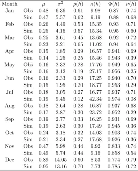
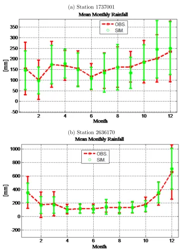
riod are compared. Results in Figure 2 and Tables 3 and 4 show that µ,σ2,ρ(h) andκ(h) seem to be well simulated. The overall observed monthly statistics show that the rainfall vari-ability in the studied stations is slightly dif-ferent where the µ ranged from 0.1 mm/h to 0.3 mm/h and 0.1 mm/h to 0.8 mm/h, respec-tively. This is probably due to geographical factor whereby station 2636170 is located at the eastern part of Peninsular Malaysia. The eastern part is more vulnerable to the north-east monsoon wind which brings heavier rain-fall to the region. Meanwhile, theσ2for station 1737001 ranged from 1.68 mm/h to 7.00 mm/h and theσ2for station 2636170 ranged from 1.85 mm/h to 14.05 mm/h. High range of variance is found at station 2636170 with 12.2 mm/h
(14.05-1.85=12.2 mm/h) as compared to sta-tion 1737001 with 5.32 mm/h (7.00-1.68=5.32 mm/h) due to high variability of monthly rain-fall in station 2636170 as compared to station 1737001. The ρ(h) for both stations seem to be fairly similar with the highest is observed at station 2636170 with a value of 0.61 and the lowest is observed at station 1737001 with a value of 0.1. This shows that both stations have positive serial correlations. As for the
κ(h), both stations are positively skewed and the skewness values are very much the same. However, the values of Φ(h) and ν(h) at sta-tions 1737001 and 2636170 ranged between 0.7 and 0.9 and between 0.4 and 0.7, respectively.
Table 4: Statistical properties at 1-hour aggregation period for Station 2636170.
Month µ σ2 ρ(h) κ(h) Φ(h) ν(h)
Jan Obs 0.48 6.36 0.61 9.98 0.87 0.74
Sim 0.47 5.57 0.62 9.19 0.88 0.68
Feb Obs 0.26 4.49 0.53 15.35 0.93 0.71
Sim 0.25 4.16 0.57 15.34 0.95 0.60
Mar Obs 0.25 3.61 0.45 13.68 0.92 0.72
Sim 0.23 2.21 0.65 11.02 0.94 0.64
Apr Obs 0.15 1.85 0.29 16.57 0.941 0.69
Sim 0.14 1.25 0.25 15.46 0.943 0.39
May Obs 0.16 2.32 0.28 17.76 0.949 0.65
Sim 0.16 3.12 0.19 27.17 0.956 0.25
Jun Obs 0.16 2.33 0.29 17.25 0.940 0.70
Sim 0.15 1.95 0.20 18.77 0.953 0.29
Jul Obs 0.18 3.05 0.27 16.77 0.937 0.71
Sim 0.19 9.45 0.12 42.34 0.974 0.08
Aug Obs 0.18 2.64 0.28 16.87 0.937 0.68
Sim 0.17 2.87 0.30 23.72 0.952 0.29
Sep Obs 0.19 2.77 0.33 16.25 0.931 0.69
Sim 0.19 2.63 0.30 17.49 0.945 0.36
Oct Obs 0.24 3.18 0.32 14.03 0.903 0.74
Sim 0.21 2.34 0.27 17.68 0.926 0.36
Nov Obs 0.47 5.98 0.44 9.92 0.833 0.74
Sim 0.49 5.74 0.44 9.16 0.858 0.54
Dec Obs 0.89 14.05 0.60 8.53 0.774 0.79
Sim 0.95 13.16 0.70 7.73 0.785 0.72
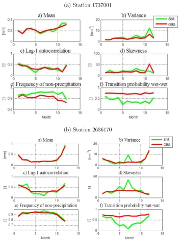
given in Figure 3, show the simulated series (green boxplot) against the observed series (red line graph). Generally, the performance of the model is quite good in mimicking the observed rainfall series with the mean of rainfall is well simulated. As seen in the figure, the peak rainfall amount for both stations occur in De-cember, followed by November. It is inter-esting to note that these months correspond to the northeast monsoon season which takes place from November to February. The re-sult is also consistent with Wong et al. (2016) where the study delineates this region based on the characteristics of rainfall. However, the maximum amount of monthly mean rain-fall for station 2636170 may reach up to 1000 mm/month whereas for station 1737001, the
(a) Station 1737001
(b) Station 2636170
Figure 2: Comparison between observed (red) and simulated (green) mean monthly statistics of hourly rainfall for (a) Station 1737001 and (b) Station 2636170.
and September/October) are influenced by the monsoon seasons (Loo et al. (2015)).
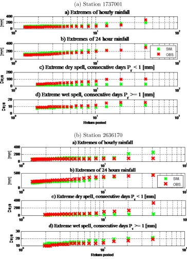
Figure 4 reveals the simulation result of ex-treme rainfall and wet/dry spell lengths for both of the stations. Both hourly and 24-hour extreme rainfall seem to be well captured by the model. Meanwhile, dry and wet spell lengths are slightly underestimated. Similarly,
(a) Station 1737001
(b) Station 2636170
Figure 3: Monthly rainfall at each station.
IV.
Conclusion
Overall, the AWE-GEN model is proven to be capable of replicating the monthly rainfall se-ries for 2 stations in Johor with Mixed Ex-ponential distribution representing the rainfall intensity. The model is able to capture the main characteristics of rainfall distribution in
(a) Station 1737001
(b) Station 2636170
Figure 4: Extremes rainfall (a) hourly (b) 24 hour and extremes spell length (c) dry consecutive days and (d) wet consecutive days.
northeast monsoon wind. The successful de-velopment of this model could be beneficial in addressing issues such as insufficiency of rain-fall data at rainrain-fall stations. In addition, the model could be employed to generate data as input to various hydrological models.
Acknowledgements
References
[1] Norzaida Abas, Zalina M Daud, and Fad-hilah Yusof. A comparative study of mixed exponential and weibull distribu-tions in a stochastic model replicating a tropical rainfall process. Theoretical and applied climatology, 118(3):597–607, 2014.
[2] Jie Chen, Fran¸cois P Brissette, and Robert Leconte. Uncertainty of down-scaling method in quantifying the impact of climate change on hydrology. Journal of hydrology, 401(3-4):190–202, 2011.
[3] Zalina Mohd Daud, Siti Musliha Mat Rasid, and Norzaida Abas. A regional-ized stochastic rainfall model for the gen-eration of high resolution data in penin-sular malaysia. Modern Applied Science, 10(5):77, 2016.
[4] Martin Dubrovsk`y, Josef Buchtele, and Zdenˇek ˇZalud. High-frequency and low-frequency variability in stochastic daily weather generator and its effect on agri-cultural and hydrologic modelling. Cli-matic Change, 63(1-2):145–179, 2004.
[5] Yusof Fadhilah, Mohd Daud Zalina, Nguyen Van-Thanh-Van, Yusop Zulkifli, et al. Stochastic modelling of hourly rain-fall processes: A comparative study using cluster point process model and markov-chain model. Proceedings of Water Down Under 2008, page 2570, 2008.
[6] Simone Fatichi, Valeriy Y Ivanov, and Enrica Caporali. Simulation of future cli-mate scenarios with a weather generator.
Advances in Water Resources, 34(4):448– 467, 2011.
[7] Hayley J Fowler, Stephen Blenkinsop, and Claudia Tebaldi. Linking climate change modelling to impacts studies: re-cent advances in downscaling techniques for hydrological modelling. International
journal of climatology, 27(12):1547–1578, 2007.
[8] Eva M Furrer and Richard W Katz. Im-proving the simulation of extreme precip-itation events by stochastic weather gen-erators. Water Resources Research, 44 (12), 2008.
[9] Muhammad Zia Hashmi, Asaad Y Sham-seldin, and Bruce W Melville. Compar-ison of sdsm and lars-wg for simulation and downscaling of extreme precipitation events in a watershed. Stochastic En-vironmental Research and Risk Assess-ment, 25(4):475–484, 2011.
[10] Zulkarnain Hassan and Sobri Harun. Im-pact of climate change on rainfall over ke-rian, malaysia with long ashton research station weather generator (lars-wg) e change on rainfall over kerian, malaysia with long ashton research station weather generator (lars-wg). Malaysian Journal of Civil Engineering, 25(1), 2013.
[11] Zulkarnain Hassan, Supiah Shamsudin, and Sobri Harun. Application of sdsm and lars-wg for simulating and downscal-ing of rainfall and temperature. Theo-retical and applied climatology, 116(1-2): 243–257, 2014.
[12] Zulkarnain Hassan, Supiah Shamsudin, and Sobri Harun. Choosing the best fit distribution for rainfall event character-istics based on 6h-ietd within peninsular malaysia. Jurnal Teknologi, 75(1), 2015.
[13] Denise E Keller. A weather generator for current and future climate conditions. PhD thesis, ETH Zurich, 2015.
[15] Chris G Kilsby, PD Jones, A Bur-ton, AC Ford, HJ Fowler, C Harpham, P James, A Smith, and RL Wilby. A daily weather generator for use in climate change studies. Environmental Modelling & Software, 22(12):1705–1719, 2007.
[16] Joo Tick Lim and Azizan Abu Samah.
Weather and climate of Malaysia. Uni-versity of Malaya Press, 2004.
[17] Yen Yi Loo, Lawal Billa, and Ajit Singh. Effect of climate change on seasonal mon-soon in asia and its impact on the vari-ability of monsoon rainfall in southeast asia. Geoscience Frontiers, 6(6):817–823, 2015.
[18] Sushant Mehan, Tian Guo, Margaret W Gitau, and Dennis C Flanagan. Compar-ative study of different stochastic weather generators for long-term climate data simulation. Climate, 5(2):26, 2017.
[19] AD Nicks, LJ Lane, and GA Gan-der. Weather generator. USDA-Water Erosion Prediction Project hillslope pro-file and watershed model documentation. NSERL Report, (10):2–1, 1995.
[20] Abas Norzaida, Mohd Daud Zalina, and Yusof Fadhilah. Application of fourier se-ries in managing the seasonality of con-vective and monsoon rainfall. Hydrolog-ical Sciences Journal, 61(10):1967–1980, 2016.
[21] Rajendra K Pachauri, Myles R Allen, Vicente R Barros, John Broome, Wolf-gang Cramer, Renate Christ, John A Church, Leon Clarke, Qin Dahe, Purna-mita Dasgupta, et al. Climate change 2014: synthesis report. Contribution of Working Groups I, II and III to the fifth assessment report of the Intergovernmen-tal Panel on Climate Change. IPCC, 2014.
[22] Clarence W Richardson. Stochastic sim-ulation of daily precipitation,
temper-ature, and solar radiation. Water re-sources research, 17(1):182–190, 1981.
[23] Clarence W Richardson and David A Wright. Wgen: A model for generating daily weather variables. 1984.
[24] Mikhail A Semenov. Simulation of ex-treme weather events by a stochastic weather generator. Climate Research, 35 (3):203–212, 2008.
[25] Mikhail A Semenov, Elaine M Barrow, and A Lars-Wg. A stochastic weather generator for use in climate impact stud-ies. User Man Herts UK, 2002.
[26] Jamaludin Suhaila, Kong Ching-Yee, Yu-sof Fadhilah, and Foo Hui-Mean. Intro-ducing the mixed distribution in fitting rainfall data. Open Journal of Modern Hydrology, 1(02):11, 2011.
[27] AH Syafrina, A Norzaida, A Kartini, and K Badron. Comparison of gamma and weibull distributions in simulating hourly rainfall in peninsular malaysia. Journal of Fundamental and Applied Sciences, 10 (3S):331–337, 2018.
[28] QJ Wang and RJ Nathan. A method for coupling daily and monthly time scales in stochastic generation of rainfall series.
Journal of Hydrology, 346(3-4):122–130, 2007.
[29] Robert L Wilby, Christian W Dawson, and Elaine M Barrow. Sdsm—a deci-sion support tool for the assessment of regional climate change impacts. Envi-ronmental Modelling & Software, 17(2): 145–157, 2002.