Spectral and Spatial Cloud Detection Onboard for
Hyperspectral Remote Sensing Image
Haoyang Li1,*, Hong Zheng1, Chuanzhao Han2, Haibo Wang3and Min Miao4
1 School of Automation Science and Electrical Engineering, Beihang University, No.37 Xueyuan Road, Beijing
100191, China; [email protected] (H.L.); [email protected] (H.Z.)
2 China Academy of Space Technology, CASA, No.104 Youyi Road, Beijing 100094, China;
[email protected](C.H.)
3 China Centre for Resources Satellite Data and Application, No.5 Fengxian East Road, Beijing 100094, China;
4 School of Mathmatics and System Science, Beihang University, No.37 Xueyuan Road, Beijing 100191, China;
[email protected] (M.M.)
* Correspondence: [email protected]; Tel.: +86-10-8231-6970
Abstract:It is strongly desirable to accurately detect the clouds in hyperspectral images onboard 1
before compression. However, conventional onboard cloud detection methods are not appropriate 2
to all situation such as shadowed cloud or darken snow covered surfaces which are not identified 3
properly in the NDSI test. In this paper, we propose a new spectral–spatial classification strategy to 4
enhance the orbiting cloud screen performances obtained on hyperspectral images by integrating 5
threshold exponential spectral angle map (TESAM), adaptive Markov random field (aMRF) and 6
dynamic stochastic resonance (DSR). TESAM is performed to classify the cloud pixels coarsely based 7
on spectral information. Then aMRF is performed to do optimal process by using spatial information, 8
which improved the classification performance significantly. Some misclassification points still exist 9
after aMRF processing because of the noisy data in the onboard environment. DSR is used to eliminate 10
misclassification points in binary labeling image after aMRF. Taking level 0.5 data from hyperion 11
as dataset, the average overall accuracy of the proposed algorithm is 96.28% after test. The method 12
can provide cloud mask for the on-going EO-1 images and related satellites with the same spectral 13
settings without manual intervention. The experiment indicate that the proposed method reveals 14
better performance than the classical onboard cloud detection or current state-of-the-art hyperspectral 15
classification methods. 16
Keywords:onboard cloud detecion; region of interest compression; themodynamic phase; spectral 17
angle map; markov random field; dynamic stochastic resonance 18
1. Introduction 19
With the development of Hyperspectral remote sensing technology, hyperspectral imaging 20
techniques have been widely used in many applications, including meteorological, earth observation, 21
military affairs, etc. Meteorological satellite has obvious advantages in monitoring the continuity, 22
spatiality and tendency of qualitative change of atmospheric environment. It provides important 23
information for the omnidirectional monitoring of atmosphere state over the entire globe. Different 24
from the concerns of meteorological satellites, earth observation satellites focus on the change of 25
earth surface, city planning, geological prospecting, military reconnaissance and natural disaster. No 26
matter what the application background is, most remote sensing images encompass the presence of 27
clouds that, especially in the visible and infrared range, strongly affect the received electromagnetic 28
radiation. Historically, clouds cover about 70% of the earth’s surface[1] and play a dominant role 29
in the energy and water cycle of our planet. But in this paper, earth’s radiative budget or aerosol 30
detection that influenced by clouds are not the main focus of our research. Typically, one hyperspectral 31
image data has over 200 spectral bands, which presents a challenge for both data transmission and 32
storage[2]. Future earth exploration missions will face unprecedented data volumes. Data size have 33
steadily increased due to improvements in detector, optics and onboard data handling technology. 34
Compared with meteorological satellite, the data size of earth observation satellite is larger due to 35
higher spatial resolution and revisiting frequency. Satellite-ground link (download speed) is more 36
tense, which can be refered to the appendix for details. Given the fact that almost all these sensors 37
have only limited memory capacity. And data transmission from the sensors to the ground become 38
inevitable for the further data analysis[3]. The large data volumes affect mission requirements for the 39
entire data handling chain, including onboard digitization, storage, downlink, ground processing, 40
and distribution[4]. Bottlenecks along this path will constrain the instrument duty cycle, reducing 41
science and application yield[5]. Depending on the application, clouds act as important information 42
for meteorological research[6][7][8] or, as unwanted corruption for earth observation[9][10]. For the 43
meteorological research users, data of image can be retained and transmitted to ground completely for 44
further research. For non-meteorological research users, as a disturbance factor for earth exploration, 45
cloud shaded the surface features who are the region of interest. As the invalid data, the data of cloud 46
region can be discarded onboard directly. They are two kinds of onboard processing strategy. 47
Data compression is necessary for onboard processing. But lossy compression methods might not 48
be suitable for hyperspectral images that are used in many accuracy demanding applications. Because 49
the images are intended to be analyzed automatically by computers[11]. Bandwidth constraints have 50
motivated new advanced lossless compression techniques such as the KLT algorithm[12][13][14] that 51
have achieved compression rates of four or greater. Efforts to optimize lossless methods eventually 52
face theoretical limits, but data size continues to increase. The challenge has driven research into 53
other techniques that can further reduce data volumes while preserving science yield. For a specific 54
application, it is very likely that only part region of the entire image carries the information of interest. 55
Rather than compressing the entire image, sometimes it just needs to compress region of interest (ROI) 56
of the image[15]. Compression methods will benefit significantly from simply not compressing those 57
invalid data regions for the sake of a higher compression ratio. Cloud region is regarded as arbitrary 58
shape of region. The ROI map will be generated to describe the shape of cloud region. And ROI map 59
can be encoded by using ARLE[16] algorithm. The ROI map with 400×256 pixels can be maximally 60
compressed into 3200bit whose compression ratio is 1:256. It is 0.002 % of the original data size, which 61
is fairly small. Excising data of cloud region before compression could significantly reduce data size. 62
However, the community lacks an accurate algorithms of real-time cloud detection in instrument 63
hardware. 64
Most onboard cloud detection methods are based on the radiometric features of clouds. The 65
“classical” cloud detection applies threshold tests to spectral properties of the image[17][18]. Pixels 66
whose values fall outside of valid ranges would be marked as clouds. For example, the algorithms that 67
are corresponding to MODIS compares the selected visible and near-infrared (VNIR) and near-infrared 68
(NIR) bands to predetermined thresholds and then aggregates the result in different combinations 69
depending on land type[19][20][21][22]. These algorithms use a combination of 14 wavelengths and 70
over than 40 tests. This underscores the intrinsic difficulty of constructing a universal and complete 71
cloud screening procedure. We focus on the visible short wave infrared (VSWIR) electromagnetic 72
spectrum from 0.4–2.5µm. There are many studies of cloud detection in these wavelengths, and 73
algorithms vary in their assumptions and complexity. Of direct relevance to this work, onboard cloud 74
detection has been demonstrated onboard the EO-1 spacecraft[23]. EO-1 cloud detection uses the 75
solar zenith angle to compute the apparent top-of-atmosphere (TOA) reflectance. Then it applies a 76
branching sequence of threshold tests based on carefully crafted spectral ratios to distinguish clouds 77
and bright landforms such as snow, ice, and desert sand. The EO-1 cloud detection also acts as a data 78
filtering step prior to onboard cryospheric and flood classification[24][25]. To our knowledge, it is the 79
only previous case of cloud screening performed on orbit. Another kind of onboard cloud detection 80
cloud contamination in acquired scenes[26][27][28]. These onboard cloud detecting methods are based 82
on threshold decision tree (TDT) in general. 83
Even more complex algorithms which belongs to ground side are proposed. Some state of-the-art 84
cloud-screening techniques estimate the optical path from absorption features such as the oxygen 85
A band, as in Gómez-Chova et al.[29] or Taylor et al[30]. Thermal infrared (TIR) channels can 86
add brightness temperature information. Minnis et al. predict clear-sky brightness temperature 87
values using ambient temperature and humidity and then excise pixels outside these intervals[31]. 88
Texture cues can be utilized to recognize clouds by their high spatial heterogeneity[32]. Martins 89
et al. demonstrated that a simple spatial analysis, i.e., the standard deviation of VNIR isotropic 90
reflectance in a 3×3 pixel window, reliably discriminated clouds from aerosol plumes over ocean 91
scenes[33]. Jin hu Bian et al. proposed spectral signature and spatio-temporal context method to 92
distinguish snow from cloud[34]. Markov random field model was developed to segment hyperspectral 93
image. Murtagh et al. represented spatial dependency by using a probabilistic Markov random field 94
prior[35]. Haoyang Yu et al. proposed adaptive MRF method combined with SVM and achieve a good 95
performance of classification of terrains[36]. Probabilistic model was another kind of cloud detection 96
method. Gómez-Chova et al. use a gaussian mixture model to produce posterior probabilities. The 97
Bayesian probabilistic model of Merchant et al. combines observational data with prior predictions 98
from atmospheric forecasts, leading to true probabilistic predictions[37]. David R proposed the 99
decision theoretic method (DTM) which was based on bayesian probabilistic model. The DTM 100
achieved negligible false positives in cloud screening[38]. Recently, deep learning was widely used in 101
classification of HSI. Li Wei et al. proposed hyperspectral image classification by using deep pixel-pair 102
features[39]. Bin Pan et al. proposed a kind of vertex component analysis network which achieved 103
better performance than some state-of-the-art method[40]. 104
TDT method have more commission errors that are at high altitudes or at low solar illumination 105
where snow was misclassified as clouds. The probabilistic model methods and the learning-based 106
methods (such as neural network or supervised learning) have more omission errors. The omission 107
errors were associated with optically thin clouds over underlying surface because of the incompleteness 108
of training sample for this kind of cloud. Focusing on these problems, our method uses exponential 109
spectral angle map, markov random field and dynamic stochastic resonance. The rest of this paper is 110
organized as follows. Section 2 introduces the problems of onboard cloud detection method in detail. 111
The proposed methodology for cloud detection is introduced in section 3. Performance evaluation for 112
different operation scenarios by using a decade-year historical image archive of the “classic” hyperion 113
spectrometer is given in section 4. Section 5 discusses the advantages, limitations and applicability of 114
the proposed method. Section 6 presents the conclusions. 115
2. Related work 116
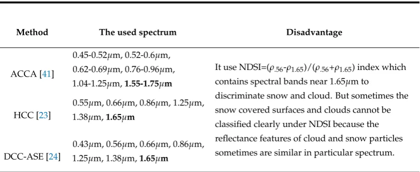
Current onboard cloud detection usually used the TDT method. The used bands of several typical 117
TDT methods are shown in table 1. All of the three TDT methods use normalized difference snow 118
index (NDSI). The NDSI test has difficulties with shadowed cloud or darken snow covered surfaces[41]. 119
And it also has difficulties with the thin cloud. One scene is shown in figure 1. Since the complexity 120
of various factors, it’s hard to classify the cloud pixels completely only in spectral feature space, as 121
shown in figure.1.(a) and (e). There are some omission errors (yellow region of figure.1.(e)) of cloud 122
detection because the optical thickness of cloud is various. The three spectral curves in figure.1.(b) 123
are sampled from three crosses marked in (a). The spectral difference between thin cloud and thick 124
cloud is obvious especially in the bands of NIR. Near 1.25µm and 1.65µm, reflectance of the thin 125
cloud is 62.2% and 14.8% of thick clouds respectively. It is because that spectrum of the thin cloud is 126
heavily affected by underlying surface. Deviation of reflectance is such huge that one set of parameters 127
is difficult to recognize various cloud completely. Commission errors also exist in cloud detection 128
(e.g. the green region in figure.1.(e)) because spectral features of cloud and snow covered surfaces 129
illumination. Figure.1.(c) shows two scenes that contain liquid cloud, mixed phase cloud, ice cloud 131
and snow. Spectral normalization of the four materials are shown in figure.1.(d). In this scene, the 132
black curve is TOA reflectance of a piece of thick ice cloud. The cyan curve is TOA reflectance of an 133
unknown portion of the mixed phase cloud where the ice phase may be dominant. The red curve 134
is TOA reflectance of a piece of liquid cloud. And the blue curve is the reflectance of snow. The 135
normalized spectrum of the three cloud types has high consistency. The biggest difference of three 136
curves is near 1.65µm. Liquid cloud has the highest reflectance near 1.65µm. But the reflectance of 137
mixed phase cloud is lower and that of ice cloud is lowest. Envelope of spectrum of snow is different 138
from spectrum of cloud near 1.03µm and 1.38µm, as shown in figure.1.(d). But reflectance of this snow 139
region is almost the same as ice cloud near 0.56µm and 1.65µm. It happens to be the spectrum that 140
are used by NDSI. For the two main existing problems of the cloud detection, figure.1.(f) symbolically 141
illustrates that cloud pixels and ground pixels cannot be separated completely under TDT classifier 142
because of the overlap of spectral features.
Table 1.Spectrum used by threshold methods and disadvantage
Method The used spectrum Disadvantage
ACCA [41]
0.45-0.52µm, 0.52-0.6µm,
0.62-0.69µm, 0.76-0.96µm,
1.04-1.25µm,1.55-1.75µm
It use NDSI=(ρ.56-ρ1.65)/(ρ.56+ρ1.65) index which
contains spectral bands near 1.65µm to
discriminate snow and cloud. But sometimes the snow covered surfaces and clouds cannot be
classified clearly under NDSI because the reflectance features of cloud and snow particles
sometimes are similar in particular spectrum. HCC [23]
0.55µm, 0.66µm, 0.86µm, 1.25µm,
1.38µm,1.65µm
DCC-ASE [24]
0.43µm, 0.56µm, 0.66µm, 0.86µm,
1.25µm, 1.38µm,1.65µm
143
The influence of clouds on solar radiation is due to reflectance, absorption and scattering of the 144
radiation by cloud particles. It depends strongly on the dimensions, opacity, thickness and composition 145
of the clouds. There are different types of clouds with different dimensions, opacity and properties 146
depending on several parameters, resulting to a different effect on solar radiation. The clouds are 147
divided into ten types as seen in table 2. Ice crystals and water drops have a different impact at the 148
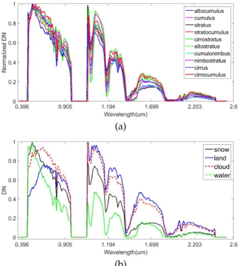
absorption and scattering of solar radiation especially in SWIR. According to statistics from 184 scenes 149
of Hyperion level 0.5 data, the solar reflectance of 10 cloud types and different ground types can be 150
seen in electromagnetic spectrum from 0.4-2.5um, as shown in figure.2. Different clouds may have 151
the different amplitude of reflectance. After normalization, the envelope of the spectral curve are 152
roughly the same, as shown in figure.2.(a). However, different surface features have different spectral 153
reflectance, as shown in figure.2.(b). In this paper, we mainly focus on how to detect cloud pixels 154
instead of recognizing different types of cloud. 155
The pure threshold method is a simple, efficient, and practical approach for cloud detection, 156
but its sensitivity to the background and the cloud condition, which makes it impractical for general 157
use[42]. Comparing with threshold method, spectral angle map (SAM) have a better cloud detecting 158
performance because of taking advantage of the more spectral information. In this paper, we 159
demonstrate a cloud-detecting algorithm which mainly uses threshold exponential spectral angle map 160
(TESAM), adaptive markov random field (aMRF) and dynamic stochastic resonance (DSR). In order to 161
get an accurate cloud cover region, we presented TESAM-aMRF-DSR method for cloud detecting. The 162
(a)
(c)
(e)
(b) (d) (f)
Figure 1.Cloud detection result under TDT method. (a) Original image; (b) spectrum of thick cloud, thin cloud and surface features that are sampled from red, blue and green cross in (a); (c) Two scenes that contain liquid cloud, mixed phase cloud, ice cloud and snow are labeled by box; (d) spectrum of liquid cloud, mixed phase cloud, ice cloud and snow that are sampled from the region in the boxes of (c) correspondingly; (e) cloud detection result under TDT method (red denotes extracted correct cloud region, yellow denotes omission errors and green denotes commission errors) (f) Diagrammatic sketch of misclassification between ground and cloud pixels under TDT method.
(a)
(b)
Table 2.Characteristic of 10 types of cloud
themodynamic phase cloud type characteristic
Water cloud
Cumulus (Cu)
They are composed of water droplets. Stratocumulus (Sc)
Stratus (St)
Cumulonimbus (Cb)
Mixed phase cloud
Altocumulus (Ac) They are composed primarily of water droplets;
however, they can also be composed of ice crystals
when temperatures are low enough. Altostratus (As)
Nimbostratus (Ns)
Ice cloud
Cirrus (Ci) They are typically thin and white in appearance, but
can appear in a magnificent array of colors when the
sun is low on the horizon. Cirrocumulus (Cc)
Cirrostratus (Cs)
3. Proposed method 164
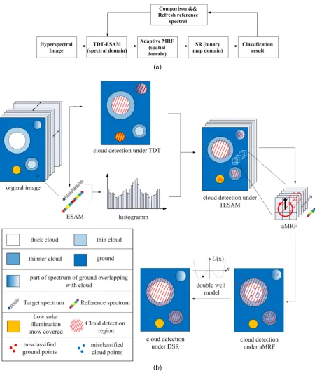
For the questions mentioned above, a new method was proposed. The general framework of the 165
proposed methods is shown in figure.3.(a). The hyperspectral images are processed by TESAM. After 166
obtaining the basic classification result from TESAM, aMRF processes based on it. Then the output of 167
aMRF is the input of DSR. Finaly, the reference spectrum is refreshed based on the final classification. 168
The flowchart of each stage is as following. TESAM is divided into two parts, TDT and ESAM. 169
The uncertainty of angle of illumination and thermodynamic phase will leads to misclassification 170
for TDT methods. Some snow covered ground and the ground whose spectrum overlaps with the 171
spectrum of cloud are misclassified as cloud under TDT, as shown in figure.3.(b). But TDT method 172
can obtain the preliminary acreage of cloud region. The ESAM can be a better calculation of the 173
distance between two spectral vectors because it is robust to illumination variations. And the ESAM 174
represents the composition of the spectral reflectance in the form of vector. It calculates the cosine 175
angle between target spectrum and reference spectrum. Then histogram can be obtained from cosine 176
angles. The preliminary acreage of cloud and the histogram jointly decide whether the pixel is 177
cloudy or not. A distinctive feature of cloudy pixel is that the non-absorbing 0.44µm-0.96µm are 178
sensitive to cloud optical thickness (COT) and most of the absorbing channels within 1.03µm-2.4µm 179
are sensitive to cloud effective particle radius (CER). TESAM tooks advantages of thses bands. The 180
misclassification reduces under TESAM. The aMRF describes the interaction between adjacent pixels 181
by using energy index. The energy is determined by spectral dimension and spatial dimension jointly. 182
Relationship of eight adjacent pixels in spatial dimension is taken into consideration. The aMRF 183
chooses 1.38µm∼1.39µm and 1.46µm∼1.55µm, which mainly takes advantage of vapor reflectance 184
bands. Although the spectrums of some thin cloud pixels and some dark cloud pixels deviate from 185
range of threshold a lot, classification result of the aMRF would not have wide range of errors. After 186
iterative processing by using minimum energy, the omission errors and commission errors both reduce. 187
The aMRF plays a role of optimization. But the onboard processing data belongs to level-0.5. This 188
indicates that the images are without radiometric calibration. Therefore, during the process of aMRF, 189
some points whose energy is mutated would be misclassified, as shown in the lower right corner 190
of figure.3.(b). These misclassified points are seemed as noisy points in binary cloud mask. DSR 191
eliminates these noisy points by using double-well model. DSR makes the isolated noisy points a 192
transition from one state to another by combining with the attributes of adjacent pixels. It plays a role 193
(a)
(b)
Figure 4.combination of ESAM with TDT.
3.1. T-ESAM 195
SAM calculates the angleθ(x,y), where x and y are N-dimensional spectral,{xi}iN=1and{yi}Ni=1, respectively,
θ(x,y) =arccos( hx,yi
kxk · kyk), 0≤θ≤ π
2 (1)
wherehx,yiis the scalar product betweenxandy
hx,yi=
N
∑
i=1
xi·yi (2)
and|| · ||means the Euclidean norm, i.e, x2
=hx,xi. Thexmeans the target spectral vector. Andy
196
means the referenced spectral vector. 197
TDT methods for cloud detection onboard such as ACCA algorithm [26] for multispectral and HCC algorithm [23] for hyperspectral appear to be good discriminators for most of the circumstance. The performance of these cloud detection algorithms are not good enough (75% of the ACCA scores were within 10% of the actual cloud cover content)[26]. This situation can be improved under SAM. And we have encapsulated the SAM metric inside an exponential function to produce ESAM function which is a positive semi-definite function. The ESAM function is defined as
ESAM(x,y) =exp(−θ(x,y)·k) (3)
where k is the gain parameters. The resolution of ESAM is getting lower when k is getting lower. 198
Generally, k is set as 0.5 (between 0 to 1). ESAM amplifies the angular distance between two vectors. 199
After the 3-D original hyperspectral imageI[L,W,H]processing by ESAM, we can obtain a 2-D computing result. The lowest value indicates most similar spectrum. These data are most likely cloud region if there are clouds in the image. Simultaneously, threshold algorithms also have detected the result of cloud region. Then we can obtain the classifier by combining ESAM with TDT, as shown in figure.4. Through TDT method, we could obtain the mumber of cloud pixels nTDTwhich is the red
solid line. The curve of cumulative frequency can be drawn when the histogram of an image has been calculated. The intersection between nTDTand curve of cumulative frequency locates the threshold
value "a" of the histogram of ESAM.
g(n)
∑
i=g(min)
histogram(ESAM(I,y) =i)≤nTDT (4)
g(n+1)
∑
i=g(min)
where "histogram(ESAM(I,y)=i)" means histogram statistics of the ESAM results between hyperspectral image and referenced spectrum that equals to “i”. The g(min)andg(n) indicate the frequencies corresponding to gray level minimum and gray levelnrespectively. Then we could obtain a classifier parameterg(n)which detects the cloud region coarsely wheng(n)satisfies equation (4) and equation (5) at the same time. The cloud detection coarse classifier is defined as
f(x) =
(
c1,i f ESAM(x,y)<g(n)
c2,i f ESAM(x,y)≥g(n) (6)
The observed spectrum of instrument data forms a vector x with multiple spectral channels per 200
pixel. The cloud-screen decision maps these pixel brightness values to a binary classificationc=f(x): 201
Rd→ {c1,c2}, where c1represents that there is a cloud present and c2represents the event that clear 202
sky is observed. Classifier f(x) detects the cloud coarsely. 203
Algorithm 1TDT assisted ESAM
Input: the remote sensing image data I with K pixels, each pixel is N-dimentional spectral vectors
X={xi}Ni=1, the referenced spectrumY={yi}iN=1 Output: the class labels mapM
step1:
for k=1 to K do
E_I=ψ(XK,Y) (ψcomputes the exponential spectral angle according to Equations(1)-(3)).
end
for k=1 to K do
nTA_I=φ(Xk)(φcomputes the number of cloud pixels according to TDT)
end step2:
Computes the histogram ofE_I step3:
for k=1 to n do
g(n)_I=Ω(E_I)(Ωcomputes the threshold for ESAM according to Equations(4)-(5)) end
Step4:
for k=1 to K do
f(x)_I=Υ(E_I)(Υdetermine the binary class label according to Equations(6)) end
3.2. aMRF model 204
The MRF model provide an accurate feature representation of pixels and their neighborhoods. The basic principle of aMRF is to spatial correlation information into the posterior probability of the spectral features. Based on the maximum posterior probability principle, the classic MRF model can be expressed as follows:
p(xi) =−
1
2ln|ΣK| − 1
2(xi−mk)
TΣ−1
K (xi−mk)−γi
∑
αi
[1−δ(ψki,ψεi)] (7)
Where mk and ΣK are the mean vector and covariance matrix of class k respectively. And the
205
neighborhood and class of pixel i are represented byεiandψkrespectively. Equation (6) separate the
206
pixels of remote sensing image into 2 classes, ground pixels and cloud pixels. The parameterγiis the
207
To obtain the local spatial weight coefficientsγi, Haoyang Yu[43] etc. used the noise-adjusted
principal components (NAPC) transform to obtain the first principal component to calculate theγi,
γi=γ0·RH Ii =γ0· vark vari
(8)
wherevark represents the class-decision variance of the neighborhood of pixel i as determined by
209
majority voting rules and vari is the local variance of pixel i [44]. When RH Ii is high, it can be
210
concluded that pixel i is located in a homogeneous region. By contrast, pixel i is on a boundary when 211
RH Iiis low. The local spatial weight coefficient whenvari=vark; usually,γ0= 1. 212
According to Equation (7), the aMRF model can be devided into two components: the energy of spectral term ai(k) and the energy of spatial term bi(k). Thus, Equation (7) can be represented in the
form
p(xi) =ai(k) +γi·bi(k) (9)
whereδ(ψki,ψεi)is the Kronecker delta function, defined as 213
δ(ψki,ψεi) =
(
1,ψki =ψεi
0,ψki6=ψεi
(10)
The pseudocode for the TESAM algorithm combined with the aMRF algorithm, abbreviated as 214
TESAM-aMRF, is shown in Algorithm 2. 215
Algorithm 2TESAM-aMRF
Input: the remote sensing image dataIwith K pixels, each pixel is n-dimentional spectral vectorsX=
{xi}ni=1, the referenced spectrumY={yi}ni=1, the class labels mapM. Output: the class labels mapM0
step1: Computes the labels mapM(results of TDT-ESAM) according to Algorithm 1; step2: Computes themkandΣkaccording to class labels map andI; (k=2);
step3: Computes thep(xi)according to Equations (7)-(10), where computing the Equations (10) with
class labels map;
step4: Refresh the class labels mapMwith minimal class ofp(xi);
step5: Iterate the procedure of step2-step4;
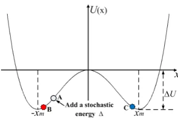
3.3. DSR model 216
The DSR model here is used to denoise the cloud mask. In analogy to Benzi’s double-well model, 217
the binary image pixel value is treated as the position of a particle in the double well. Addition of 218
stochastic energy effects its transition to the strong signal state, just as a particle makes a transition 219
from one well to another. Such a change of state of pixel under noise can be modelled by Brownian 220
motion of a particle placed in a double-well potential system shown in figure.5. The particle A is 221
located in the left well. The state of particle A may or may not turn over in the double well after giving 222
a sochastic energy to A. The location of particle A may be at ponit B if it does not turn over. And the 223
location may be at point C if it turns over. The left and the right well represents black and white pixel 224
of binary cloud mask respectively. 225
A classic 1D nonlinear dynamic system that exhibits SR is modelled with the help of the Langevin equation of motion is given below
m·d 2x(t)
dt2 +γ· dx(t)
dt =− dU(x)
dx + √
Figure 5.SR in double-well potential valley.
This equation describes the motion of a particle of mass m moving in the presence of friction,γ. 226
The restoring force is expressed as the gradient of some bistable potential function U(x). In addition, 227
there is an additive stochastic forceξ(t)of intensity D. 228
If the system is heavily damped, the inertialmd2dtx(2t)term can be neglected. Rescaling the system
in (11) with the damping termγgives the stochastic overdamped Duffing equation, which is frequently used to model non-equilibrium critical phenomena as given in (12)
dx(t) dt =−
dU(x) dx +
√
D·ξ(t) (12)
where U(x) is a bistable quartic potential given in
U(x) =−a· x 2
2 +b· x4
4 (13)
Here, a and b are positive bistable double-well parameters. The double-well system is stable 229
atxm = ± q
a
b separated by a barrier of height∆U = a 2
4b whenξ(t)is zero. The Langevin equation
230
describes the motion of particle in a general double-well.
Algorithm 3aMRF-DSR
Input: the class labelsM0 Output: the class labelsMf inal
step1:
for k=1 to K do
Ck=ζ(M0(k)=cloud),Gk=ζ(M0(k)=ground) (ζcomputes the pixel number of 8-neighborhood around pixel k that belongs to ground and cloud respectively);
compareCkandGk, designating the number of bigger one toξ(t);
Refresh x according to Equations (12)-(13); end
step2: RefreshM0
step3: Iterate the procedure of step1-step2;
231
4. Method Feasibility Validation 232
4.1. Dataset 233
In this section, we evaluate the performance of the proposed algorithms by using the widely used 234
hyperspectral data from hyperion sensor of EO-1. The data used in onboard processing is level 0.5. And 235
(a)
(b)
(c)
(d)
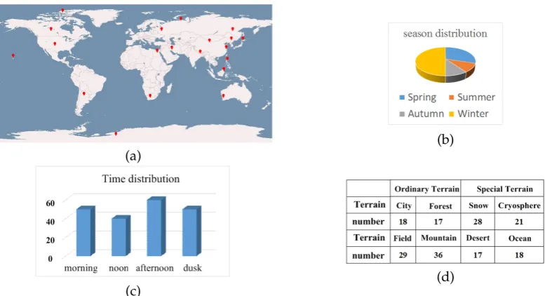
Figure 6. Test dataset description. (a) Geographical distribution of the selected scene; (b) Season distribution of the selected scene; (c) Time distribution of the selected scene; (d) Scene number of each terrain.
range, desert, snow and cryosphere. The span of time contains spring, summer, autumn, winter, 237
morning, noon and dusk of recent decade year. The span of latitude contains tropical, subtropical, 238
temperate, frigid and polar zone. Geographical distribution of the selected scenes is spread all over 239
the world. Season distribution is at all seasons but mainly focusing on winter. Statistics of test dataset 240
is shown in figure.6. 241
In meteorological research, clouds are labeled pixel by pixel through particle scattering models. 242
The single scattering properties of liquid water clouds are calculated from Mie theory[48] and are 243
integrated over a Modified Gamma droplet size distribution. The single scattering properties of ice 244
clouds are obtained from Yang et al[49]. Computed single scattering properties (single scattering 245
albedo, asymmetry parameter, extinction efficiency, phase function) for both ice and liquid water clouds 246
are stored in the LUT. However, for earth observed satellite, resolution is higher than meteorological 247
satellite. Particle scattering models can’t guarantee that each cloud pixel has been labeled just through 248
the spectrum. The groundtruth of cloud is that manual label uses Visual Cloud-Cover Assessment 249
method (VCCA). This method was used as a measure of the true cloud cover in the scene. The magic 250
wand and freehand lasso tools of Photoshop were used to isolate clouds. The wand employs a seed-fill 251
threshold algorithm to compute regions of brightness similarity based on a mouse click of a single 252
pixel. The algorithm compares the selected pixel’s brightness values to all other pixels and retains 253
those within a selectable tolerance threshold. Additional cloud pixels are added by using the wand 254
repeatedly until the cumulative selection of visible clouds had essentially zero possibility of VCCA 255
omission errors. Snowfields and other unwanted bright features were then manually subtracted 256
using the lasso tool to reduce VCCA commission errors. All these works were done by well-trained 257
professional persons. After the VCCA scores were established, the result was a binary cloud mask 258
that allowed a cloud cover percentage computation that served as the cloud “truth” for validating the 259
accuracy of our proposed method. The uncertainty of manual labeling is the border of thin cloud and 260
the cirrus which is floating on the snow especially in visible bands. Therefore, it is necessary to use 261
infrared bands to label cloud pixels in assistant, but choosing which bands to separate cloud pixels 262
4.2. Accuracy Accessment 264
The following three different accuracies measures, which were the overall accuracy, precision and recall, were used to assess the accuracy of the algorithm results. Define the True Positive (TP) as the pixel-number of clouds correctly labeled as belonging to clouds in the algorithm, False Negatives (FN) as the pixel-number of clouds incorrectly labeled as belonging to non-cloud, and True Negatives (TN) as pixel-number of non-cloud which also labeled as belonging to non-cloud. The accuracy, precision and recall are then defined as
Recall=TP/(TP+FN) (14)
Precision=TP/(TP+FP) (15)
FPR=FP/(FP+TN) (16)
In the cloud case, precision denotes the proportion of correctly detected cloud pixels in the cloud 265
detection results, while recall is of all pixels that are actually clouds in the image, what fraction of 266
them were detected as clouds. For precision and recall, they are better reflects the errors of cloud 267
classification than overall accuracy. 268
4.3. Detection results 269
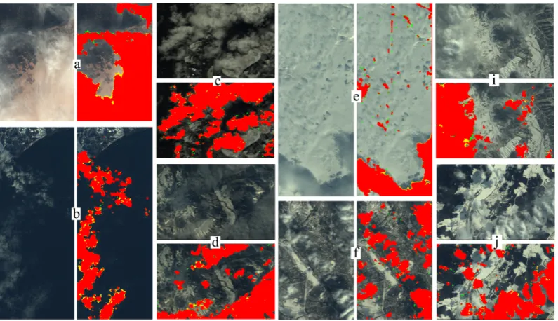
Figure.7 shows the cloud detection results for different terrains. Just by visually comparing the 270
results with the false color composites, it is clear that the algorithm developed in this study achieves 271
good performance in detecting the cloud pixels. Figure.7.(a) was a summer image acquired on 8th
272
August 2013 with cirrostratus over the desert. The detection result indicates that algorithm showed its 273
strong ability in excluding the cloud from desert even if cloud is such thin that spectrum of cloud is 274
mixed with spectrum of desert pixels. On the other hand figure.7.(b) was a winter image acquired on 275
3rdJune 2013 with dark stratus over the ocean and coast. Clouds contain water droplets that have the 276
same materials of ocean in this season. However, water of the ocean is in liquid and water of clouds 277
is in form of aerosol. Even if the spectrum of the same materials is different due to different forms 278
or temperature. About 1.73% omission errors, the yellow region, which is different from manually 279
labeled cloud mask exist on the border of thin cloud. Figure.7.(c) was a spring image acquired at noon 280
on 22thMay 2012 with cumulus and stratocumulus around Himalaya mountains. And figure.7.(d) 281
was a winter image acquired at dusk on 3rdJanuary 2007 with altocumulus over mountain with 0.62% 282
omission errors. Comparing figure.7.(c) with figure.7.(d), cloud of the former seems lighter than the 283
later due to smaller sun zenith angle. But both the two image have good cloud detection result even if 284
the darker cloud can be also detected. Figure.7.(f) was a winter image acquired on 28thMarch 2005 285
with cumulus over the city Haerbin. About 0.23% commission errors that both freezing river and 286
city highlights are classified into cloud. About 0.16% omission errors exist in suspected cloud region. 287
Figure.7.(e), figure.7.(i) and figure.7.(j) are both clouds over the snow or ice. Figure.7.(e) was an image 288
acquired on 12thMay 2012 with stratocumulus over snowfield in the cryosphere. The cloud pixels, 289
about 4.8% pixels of the whole image, are indistinguishable by naked eyes. These pixels are floating 290
over the snow field. There are 0.41% commission errors when compared with manually labeled cloud 291
mask. Figure.7.(i) was a spring image acquired on 17thMarch 2007 with altostratus over mountain 292
which is covered by snow. The edge of altostratus looks similar to ground because it doesn’t have a 293
clear outline in visible bands. Although there are 2.97% cloud pixels that are hard to be distinguished 294
by eyes in visible bands, they were classified by the proposed method correctly. Figure.7.(j) was a 295
spring image acquired on 28thMarch 2005 with cumulus over the forest which is covered by some 296
frozen lake. Most of the cumulus are floating on the ice. They have 0.21% omission errors. 297
4.4. Performance of Each Stage for the Cloud Detection 298
Figure.8 provides an illustration of the algorithm performance for the each processing stage. It 299
Figure 7.Cloud detection results for different kinds of ground. (a) Desert with thin cirrostratus and cloud detection result; (b) Ocean with dark stratus and cloud detection result; (c) Mount Qomolangma with stratocumulus and cloud detection result; (d) Mountain with dark altocumulus and cloud detection result; (e) Snow cover with straocumulus and cloud detection result; (f) Highlight city with frozen lake scene and cloud detection result; (i) Mountain with thin altostratus and cloud detection result; (j) Frozen field with cumulus and cloud detection result. (Red denotes extracted correct cloud regions (TP), yellow denotes missed cloud regions (omission errors/FN) and green denotes non-cloud regions misjudged as cloud regions (commission errors/FP))
the results with the false color composites, it is clear that there are FN classifications in light cloud 301
region under TDT method because of the unsuitable and fixed parameters for various reflectance as 302
shown in figure.8.(h). Contrarily, TESAM could classified the cloud regions that are misclassified under 303
TDT method correctly, as shown in figure.8.(i). And under TESAM, the various reflectance didn’t 304
have much influence over cloud detection. Comparing with TDT, TESAM seems to be conservative, 305
abstaining ambiguous classification to prevent mixture of heterogeneous spectrum for the aMRF 306
procedure. The ambiguous classification is shown in the yellow circle of figure.8.(k). These region are 307
not labeled as cloud under TESAM, as shown in figure.8.(l). After TESAM detecting, the cloud regions 308
detected by TESAM work as a role of seed regions in the procedure of aMRF. By comparing yellow 309
circles of figure.8.(d) and figure.8.(e), we can see that after aMRF detecting, some cloud regions grow 310
more full. And TN regions have been recovered to ground pixels because the aMRF has fault-tolerant 311
ability. The detailed iterative process of aMRF will be introduced later. But the spectrum of some 312
individual pixels still has the strong similarity with cloud under the selected bands for aMRF. Therefore, 313
even if considering the neighbors’ contribution, the energy of these pixels under aMRF is still low. 314
They were misclassified as cloud pixels. However, these pixels of cloud mask are seemed as noisy 315
points for DSR. By comparing figure.8.(m) and figure.8.(n), DSR turned the binary properties of these 316
noisy points over. The vertical line and some isolate pixels in figure.8.(m) have been eliminated after 317
DSR processing, as shown in figure.8.(n). 318
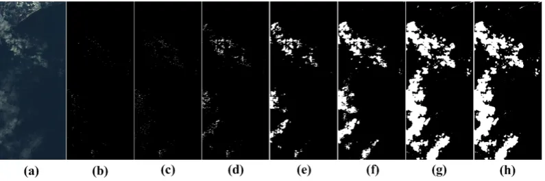
The detailed example for iterative process of aMRF is shown in figure.9. The cloud regions that 319
are detected by TDT method and TESAM are rather limited (0.02% and 0.12% of TP were within 320
18.3% of the actual cloud cover content). Only a few detected cloud pixels existed in the mask, as 321
seen in figure.9.(a) and (b). The detection result of TESAM is treated as initial classification for aMRF. 322
Comparing figure.9.(c-h), obviously, aMRF method have strong robustness if the spectrum of the initial 323
Figure 8.Comparison of cloud detection results. (a) A winter image acquired at 7 December 2013 with obvious clouds over the whole image; (b) Result of manually labeled image; (c) Cloud detection result by using TDT method; (d) Cloud detection result by using TESAM method; (e) Cloud detection based upon (d) by using aMRF method; (f) Cloud detection based upon (e) by using DSR; (g), (h) and (i) are origin picture, TDT labeled and TESAM labeled of cloud region respectively. (g), (h) and (i) are corresponding to the red box in (a), (c), (d) respectively; (j), (k) and (l) are corresponding to origin picture, TDT labeled and TESAM labeled of cloud region respectively. (j), (k) and (l) are corresponding to the orange box in (a), (c), (d); (m) is the result of aMRF processing, which is corresponding to purple box in (e); (n) is processed by DSR based on (e), which is corresponding to purple box in (f).
previous iteration. And after 8th iteration, classification has good agreement with the real cloud region. 325
And this image tended to be convergent at the 16thiteration. 326
Figure.10 shows comparison of cloud detection performance of some methods. The terrains 327
from the first row to the last row are ocean, mountain, city, desert, ice and cryosphere. It can be 328
observed that the proposed method produced the best precision ratio and recall ratio and its error 329
was lower than that of the other methods. ACCA have high FN for ordinary terrain and high FP for 330
special terrain due to lacking the thermal infrared band. HCC has difficulty in detecting thin or dark 331
cloud. Decision Theoretical Method(DTM) classifies majority of thin clouds into ground. It is with 332
high FP under DTM. The support vector machine adaptive markov random field (SVM-aMRF) and 333
rolling guidance filter and vertex component analysis network(R-VCANet) have higher recall ratio 334
and precision ratio than the previous two. But they still have some classification error for thin clouds 335
that mainly because thin clouds are mixed with other spectrum that can’t be learned sufficiently. ROC 336
curve and precision/recall curve can be seen in figure.11 and figure.12. 337
5. Discussions 338
5.1. The Effectiveness of Combining Threshold Decision Tree and Spectral Angle Map 339
Spectral Angle Map is widely used due to its simplicity and geometrical interpretability. SAM is 340
invariant to (unknown) multiplicative scalings of spectra due to differences in illumination and angular 341
orientation. One of the most important properties of the spectral angle distance is the invariance to 342
multiplicative scaling. Due to the invariant nature of the angle among the linearly scaled variations, 343
the spectral angle between two pixels is more sensitive to the pattern (shape) of the spectral signatures 344
instead of absolute intensities. Traditional TDT methods sometimes overestimate or underestimate the 345
cloud region because the fixed parameters were inappropriate to the variant illumination and angular 346
orientation. In theory, TESAM method could reduce the misclassification error. 347
5.2. The Useness of Spatial Information for Cloud Detection 348
For still existing wrong classification pixels after TESAM, aMRF was used to synthesize all 349
the spectral and spatial information into an energy index to find the class attribute at the regional 350
scales. In general, it achieved the optimal status when the energy was stable, then the iteration 351
procedure terminated. The aMRF mainly choose the bands of vapor reflection (1.38µm∼1.39µm and 352
1.46µm∼1.55µm). Spectrums of thin cloud pixels and dark cloud pixels deviate threshold a lot. But 353
aMRF can recognize these cloud pixels again. The cloud mask resulted from aMRF contains noisy 354
points because the data processed onboard belongs to level 0.5 that are not fully calibrated. The 355
radiance and reflectance of values for SWIR bands of level 0.5 should be considered as pseudo-radiance 356
and pseudo-reflectance. DSR can eliminate these noisy points of binary mask. It is a refinement process 357
for cloud detection. Figure.12 shows that the over all accuracy of aMRF iteration results and DSR 358
iteration results. We randomly selected parts of the dateset. Over all accuracy of each aMRF iteration 359
results is shown in figure.12.(a). The 0thiteration means over all accuracy after TESAM. During the 360
aMRF iteration, the accuracy of each time increased more or less. The final performance of improved 361
accuracy with aMRF iteration are not all the same because it mainly depends on cloud condition. The 362
convergence criterion for aMRF iteration is that class attribute of 0.5% pixels won’t change between 363
two adjacent iterations. And the over all accuracy of each DSR iteration results is shown in figure.12.(b). 364
The 0thiteration means over all accuracy after aMRF. During the DSR iteration procedure, the accuracy 365
of each time numerically increased little. But it eliminates many isolated noise-points, which are greatly 366
beneficial to ROI compression. The convergence criterion for DSR iteration is that class attribute of 367
0.01% pixels won’t change between two adjacent iterations. 368
5.3. Error Sources of the proposed Method 369
In brief, the cloud detection results indicated that the proposed method has a good performance 370
for the detecting cloud in EO-1 images. However, two error sources which might influence the 371
algorithm accuracy should also be pointed out. The first error source came from the way that the cloud 372
region detected by TDT algorithm is bigger than actual size. That’s probably because of unsuitable 373
parameters. Correspondingly, TESAM will overestimate cloud areas because size of cloud region is 374
decided by TDT and histogram of TESAM together. In this condition, it will increase FPR region of 375
TESAM results. Because the impure cloud spectrum may lead to error classification of large area under 376
aMRF. The second error is that the selected bands for aMRF may not be optimal for all kinds of surface 377
features. In this case, the advantages of seed region are losed if the contribution from the weight of 378
Origin ACCA HCC SVM-aMRF R-VCANet TESAM-aMRF-DSR
(a) (b)
Figure 11.Comparison of performance about the different algorithms. (a)ROC curve of cloud detection performance for each method. (b)Precision performance curve corresponding to Recall for each method.
(a)
(b)
Figure 13.Statistics of cloud cover and ratio of compression quantity between filling and non-filling cloud regions.
5.4. Effect of compression based on cloud detection 380
The compression effect is worth mentioning. The cloud region is filled with special value after 381
obtaining the cloud mask. Then the data of cloud region can be removed through compression. For a 382
scene with 30.12% cloud cover rate of hyperion image, data size of the filled-value one is 71.27% of the 383
original one that both of them have been processed by lossless compression. One hand, it is necessary 384
to consider the difference of lossless compression ratio between ground and cloud. On the other hand, 385
the non-filling cloud’s contribution to compression is not as much as the filling cloud’s. The statistics of 386
cloud cover and ratio of compression quantity between filling and non-filling cloud regions is shown 387
in figure 13. The regression line is shown that the ratio of compression quantity between filling and 388
non-filling cloud regions is approximately proportional to the cloud cover ratio. The tendency is linear. 389
And the closer to 1:1 they are, the better compression performance of filling-value it is. Some points 390
that are higher than 1 means that the scene contains little thin cloud. Some points that are close to zero 391
indicate that the scene is totally covered by cloud. 392
5.5. Applicability of the Developed Methods in the Feature 393
The proposed method is highly automatic and efficient when processing a tremendously large 394
volume of imagery real-time. It can be easily implemented on a parallel processor, such as FPGA. 395
The proposed method needs some external storage devices or the architectures such as ping-pong 396
structure. Because it could restore data for supporting the use of spatial context. Moreover, 397
classifiers instantiated in hardware logic typically have already achieved in the implementation 398
of arccosine[45], exponentials[46][47] functions, and even floating-point operations, supporting many 399
nonlinear classifiers and naive implementations of linear classifiers. Additionally, there are real-time 400
requirements for processing procedure. Bandwidth of multi DDRs could satisfy Gb/s throughput of 401
algorithm by using a small fixed number of arithmetic operations on locally available data. It also can 402
be adapted for images acquired by similar satellite instruments, which have similar spectral bands and 403
temporal resolutions. The method in this paper is general and efforts in the future will be put into the 404
6. Conclusions 406
The TESAM-aMFR-DSR is an innovative approach for onboard cloud detection. Different from 407
classical hyperspectral cloud detection algorithm, the proposed method combines TDT with ESAM. 408
As initial seed region of cloud for aMRF, it improves spectral purity. The aMRF method uses energy 409
index by combining spectral features with spatial information. It is robust to the shadowed region 410
of cloud area, the thin cloud and the misclassified ground pixels. There are noisy points that are 411
misclassified during aMRF process because of not fully calibrated onboard processing data. Then DSR 412
eliminated these noisy points by using double-well model. The cloud detecion results obtained in 413
this study demonstrate the performance of the proposed method. The performances of this method 414
are evaluated using EO-1/Hyperion images. Agreements were found between detection results and 415
manually labeled image with the over all accuracy 96.28%. The spatial information can approximately 416
exclude misclassified 8.35% cloud pixels from initial spectral tests. The ratio of compression quantity 417
between filling scenes and non-filling scenes is approximately proportional to the cloud cover ratio. 418
The tendency is linear. The filling cloud regions improve compression performance. In conclusion, 419
the proposed method exhibited high accuracy for clouds recognition of EO-1 Hyperion images and 420
was an improvement over the traditional spectral-based algorithms. The proposed method also can be 421
adapted for images acquired by similar satellite instruments, which have similar spectral bands and 422
temporal resolutions. 423
Acknowledgments:Project supported by the National Nature Science Foundation of China(No.60543006). The 424
authors would like to thank the editor and reviewers for their instructive comments that helped to improve this 425
manuscript. Besides, they would also like to thank the international scientific data service platform and the U.S. 426
Geological Survey website 427
Author Contributions:Haoyang Li, Hong Zheng and Chuanzhao Han conceived of the study and designed the 428
experiments; Haibo Wang and Min Miao took part in the research and analyzed the data; Haoyang Li wrote the 429
main program and most of the paper. 430
Conflicts of Interest:The authors declare no conflict of interest. 431
Abbreviations 432
The following abbreviations are used in this manuscript: 433
ACCA Automatic Cloud Cover Algorithm aMRF adaptive Markov Random Field
CC Cloud Cover
DCC-ASE Detection of Cryospheric Change Automonous Sciencecraft Experiment DSR Dynamic Source Resonance
DTM Decision Theoretic Method EO-1 Earth Observing-1
ESAM Exponential Spectral Angle Map FL Fast Lossless
FN False Negative FP False Positive FPR False Positive Rate HCC Hyperion Cloud Cover HSI Hyperspectral Image LUT Look Up Table MRF Markov Random Field
MODIS Moderate-resolution Imaging Spectroradiometer NAPC Noise-adjusted Principle Components
NDSI Normalized Difference Snow Index NIR Near Infrared
ROC Receiver Operating Characteristic Curve ROI Region of Interest
R-VCANet Rolling Guidance filter and Vertex Component Network SAM Spectral Angle Map
SVM Support Vertor Machine
SVM-aMRF Support Vector Machine adaptive Markov Random Field TDT Threshold Decision Tree
TESAM Threshold assisted Exponential Spectral Angle Map TIR Thermal Infrared
TN True Negative
TOA Top of Atmosphere TP True Positive
USGS United States Geological Survey VNIR Visible and Near Infrared VSWIR Visible and Short Wave Infrared 435
Appendix A 436
437
1. GEWEX, http://climserv.ipsl.polytechnique.fr/gewexca/ 438
2. Hongda Shen; W. David Pan; Dongsheng Wu, Predictive lossess compression of regions of interest in 439
hyperspectral images with no-data regions. IEEE Trans. Geosci. Remote Sens.201655, 173-182. 440
3. Hongda Shen; W. David Pan; Dongsheng Wu, Predictive Lossless Compression of Regions of Interest in 441
Hyperspectral Image Via Correntropy Criterion Based Least Mean Square Learning. In proceedings of IEEE 442
International Conference on Image Processing, Phoenix, Arizona, USA, 25-28 Sept 2016. 443
4. L. Mandrake; C. Frankenberg; C. W. O’Dell; G. Osterman; P. Wennberg; D. Wunch, Semi-autonomous 444
sounding selection for OCO-2. Atmosp. Meas. Tech. Discuss.2013,6, 5881–5922. 445
5. L. S. Chien; D.Mclaren; D. Tran; A. G. Davies; J. Doubleday; D. Mandl, Onboard product generation on earth 446
observing one: A pathfinder for the proposed HyspIRI mission intelligent payload module. IEEE JSTARS. 447
2013,6, 257–264. 448
6. Xiangxin Xu; Chunqiang Yuan; Xiaohui Liang; Xukun Shen, Rendering and Modeling of Stratus Cloud 449
Using Weather Forecast Data. In Proc. Int. Conf. on Virtual Reality and Visualization, Fujian, China, 17-18 450
Table A1.Meteorological satellite VS Earth observation satellite
Satellite The used sensor Image resolution Data size Download speed
Meteorological
satellite
FY-3A MERSI 1100m 4GB 93Mb/s
Noaa18 AVHRR 1100m / 138Mb/s
GMS-5 VISSR 1250m / 14Mb/s
Meteosat VISSR 1000m / 3.2Mb/s
Meteor-m2 KMSS 1000m / 665kb/s
Earth
observation
satellite
EO-1 Hyperion 30m / 120Mb/s
NEMO(HRST) AVIRIS 20m 227GB 150Mb/s
QuickBird QuickBird 0.6m 128GB 320Mb/s
LANDSAT8 OLI/TIRS 15m 400GB 330Mb/s
EROS B1 Panchromatic 0.82m / 280Mb/s
Resurs dk1 ESI 1m 768GB 330Mb/s
7. M. King, S. Platnick, W. Menzel, S. Ackerman, and P. Hubanks; M. Chodas, Spatial and temporal distribution 452
of clouds observed by MODIS onboard the Terra and Aqua satellites. IEEE Trans. Geosci. Remote Sens. 453
2013,51, 3826–3852. 454
8. E. Cadau; G. Laneve, Improved MSG-SEVIRI images cloud masking and evaluation of its impact on the fire 455
detection methods. In Proc. IGARSS, Massachusetts, U.S.A., 6-11 July 2008. 456
9. Hongda Shen; W. David Pan; Yi Wang, A Novel Method for Lossless Compression of Arbitrarily Shaped 457
Regions of Interest in Hyperspectral Imagery. In Proc. IEEE Southeast Con, Florida, USA, 9 - 12 April 2015. 458
10. M. Mercury; R. Green; S. Hook; B. Oaida; W. Wu; A. Gunderson; M. Chodas, Global cloud cover for 459
assessment of optical satellite observation opportunities: A HyspIRI case study. Remote Sens. Environ.2012, 460
126, 62–71. 461
11. Marco Conoscenti; Riccardo Coppola; Enrico Magli, Constant SNR, Rate Control, and Entropy Coding for 462
Predictive Lossy Hyperspectral Image Compression. IEEE Trans. Geosci. Remote Sens.2016,54, 7431-7441. 463
12. Noor. NRM ; Vladimirova. T, Investigation into lossless hyperspectral image compression for satellite remote 464
sensing. International Journal of Remote Sensing.2013,34, 5072-5104. 465
13. Nian Yongjian; Xu Ke; Wan Jianwei, Block-based KLT compression for multispectral images. InternationalJ. 466
of Wavelets Multiresolution and Information Processing.2016,14. 467
14. Wang L; Wu JJ; Jiao LC; Shi GM, Lossy-to-Lossless Hyperspectral Image Compression Based on Multiplierless 468
Reversible Integer TDLT/KLT. IEEE Geoscience and Remote Sensing Letters.2009,6, 587-591. 469
15. J. Gonzalez-Conejero; J. Bartrina-Rapesta; J. Serra-Sagrista, JPEG 2000 encoding of remote sensing 470
multispectral images with no-data regions. IEEE Geosci. Remote Sens. Lett.2010,7, 251 – 255. 471
16. Haoyang Li; Hong Zheng; Chuanzhao Han, Adaptive run-length encoding circuit based on cascaded 472
structure for target region data extraction of remote sensing image. In Proc. International Conference on 473
Integrated Circuits and Microsystems, Chengdu, China, 25-28 November 2016. 474
17. E. El-Araby; M. Taher; T. El-Ghazawi; J. Le Moigne, Prototyping automatic cloud cover assessment (ACCA) 475
algorithm for remote sensing on-board processing on a reconfigurable computer. IEEE International 476
Conference on Field-Programmable Technology. Singapore, Singapore, 11-14 Dec. 2005. 477
18. Gao, X.J.; Wan, Y.C.; Zheng, X.Y, Real-Time automatic cloud detection during the process of taking aerial 478
photographs. Spectrosc. Spectr. Anal.2014,34, 1909–1913. 479
19. S. A. Ackerman; K. I. Strabala; W. P. Menzel; R. A. Frey; C. C. Moeller; L. E. Gumley, Discriminating clear sky 480
from clouds with MODIS.J.Geophys. Res. Atmosp.1998,103, 32141–32157. 481
20. S. Ackerman; R. Holz; R. Frey; E. Eloranta; B. Maddux; M. McGill, Cloud detection with MODIS. Part II: 482
21. R. A. Frey; S. A. Ackerman; Y. Liu; K. I. Strabala; H. Zhang; J. R. Key; X. Wang, Cloud detection with MODIS. 484
Part I: Improvements in the MODIS cloud mask for collection 5. J.Atmosp. Ocean. Technol.,2008,25, 485
1057–1072. 486
22. Jing Wei; Lin Sun; Chen Jia; Yikun Yang; Xueying Zhou; Ping Gan; Shangfeng Jia; Fangwei Liu; Ruibo 487
Li, Dynamic threshold cloud detection algorithms for MODIS and Landsat 8 data. IEEE International 488
Geoscience and Remote Sensing Symposium, Beijing, China, 10-15 July 2016. 489
23. M. K. Griffin; H. K. Burke; D. Mandl; J. Miller, Cloud cover detection algorithm for EO-1 hyperion imagery. 490
in Proc. 17th SPIE AeroSense Conf. Algorithms Technol. Multispectral, Hyperspectral Ultraspectral Imagery 491
IX, Orlando, FL, USA, 21-25 July 2003. 492
24. T. Doggett; R. Greeley; S. Chien; B. Cichy; A. Davies; G. Rabideau; R. Sherwood; D. Tran; V. Baker; J. Dohm; 493
F. Ip, Autonomous on-board detection of cryospheric change with Hyperion on-board Earth Observing-1. in 494
Remote Sens. Environ.2006,101, 447–462. 495
25. F. Ip; J. Dohm; V. Baker; T. Doggett; A. Davies; R. Castao; S. Chien; B. Cichy; R. Greeley; R. Sherwood; D. 496
Tran; G. Rabideau, Flood detection and monitoring with the autonomous sciencecraft experiment onboard 497
EO-1. Remote Sens. Environ.2006,101, 463–481. 498
26. Richard R. Irish., Landsat 7 automatic cloud cover assessment. Algorithms for Multispectral, Hyperspectral, 499
and Ultraspectral Imagery, Proceedings of SPIE, Orlando, FL USA, 24, April, 2000. 500
27. M. Wang; W. Shi, Cloud masking for ocean color data processing in the coastal regions. IEEE Trans. Geosci. 501
Remote Sens.2006,44, 3105–3196. 502
28. Juan Deng, Hongchen Wang, Jun Ma, An Automatic cloud detection algorithm for Landsat Remote Sensing 503
Image. 4th International Workshop on Earth Observation and Remote Sensing Applications, Guangdong, 504
China, 11-14 Dec. 2016. 505
29. L. Gómez-Chova; G. Camps-Valls; J. Calpe-Maravilla; L. Guanter; J. Moreno, Cloud-screening algorithm for 506
ENVISAT/MERIS multispectral images. IEEE Trans. Geosci. Remote Sens.,2007,45, 4105–4118. 507
30. T. Taylor; C. O’Dell; D. O’Brien; N. Kikuchi; T. Yokota; T. Nakajima; H. Ishida; D. Crisp; T. Nakajima, 508
Comparison of cloud-screening methods applied to GOSAT near-infrared spectra. IEEE Trans. Geosci. 509
Remote Sens.,2012,50, 295–309. 510
31. P. Minnis; Q. Z. Trepte; S. Sun-Mack; Y. Chen; D. R. Doelling; D. F. Young; D. A. Spangenberg; W. F. Miller; B. 511
A. Wielicki; R. R. Brown; S. C. Gibson; E. B. Geier, Cloud detection in nonpolar regions for CERES using 512
TRMM VIRS and terra and aqua MODIS data. IEEE Trans. Geosci. Remote Sens.,2008,46, 3857–3884. 513
32. J. Lee; R.Weger; S. Sengupta; R.Welch, A neural network approach to cloud classification. IEEE Trans. Geosci. 514
Remote Sens.,1990,28, 846–855. 515
33. J. V. Martins; D. Tanré; L. Remer; Y. Kaufman; S. Mattoo; R. Levy, MODIS cloud screening for remote sensing 516
of aerosols over oceans using spatial variability. Geophys. Res. Lett.,2002,29, MOD4-1–MOD4-4. 517
34. Jinhu Bian; Ainong Li; Qiannan Liu; Chengquan Huang, Cloud and Snow Discrimination for CCD Images 518
of HJ-1A/B Constellation Based on Spectral Signature and Spatio-Temporal Context. Remote Sensing,2016, 519
8, 1-31. 520
35. F. Murtagh, D. Barreto, and J. Marcello, Decision boundaries using Bayes factors. IEEE Trans. Geosci. Remote 521
Sens.,2003,41, 2952–2958. 522
36. Haoyang Yu; Lianru Gao; Jun Li; Shansan Li; Bing Zhang, Spectral-Spatial Hyperspectral Image Classification 523
Using Subspace-Based Support Vector Machines and Adaptive Markov Random Fields. Remote Sensing., 524
2016,8, 1-21. 525
37. C. Merchant, A. Harris, E. Maturi, and S. MacCallum, Probabilistic physically based cloud screening of 526
satellite infrared imagery for operational sea surface temperature retrieval. Q. J. R. Meteorol. Soc.,2005,131, 527
2735–2755. 528
38. David R. Thompson; Robert O. Green; Didier Keymeulen; Sarah K. Lundeen; Yasha Mouradi; Daniel Cahn 529
Nunes; Rebecca Castaño; Steve A. Chien, Rapid Spectral Cloud Screening Onboard Aircraft and Spacecraft. 530
IEEE Trans. on Geosci. and Remote Sens.,2014,52, 6779 - 6792. 531
39. Li Wei; Wu Guodong; Zhang Fan; Qian Du, Hyperspectral Image Classification Using Deep Pixel-Pair 532
Features. IEEE Trans. on Geosci. and Remote Sens.,2017,55, 645-657. 533
40. Bin Pan; Zhenwei Shi; Xia Xu, R-VCANet: A New Deep-Learning-Based Hyperspectral Image Classification 534
Method. IEEE Journal of Selected Topics in Applied Earth Observations and Remote Sensing,2017,10, 1975 535
41. Pasquale L. Scaramuzza; Michelle A. Bouchard; John L. Dwyer, Development of the Landsat Data Continuity 537
Mission Cloud-Cover Assessment Algorithms. IEEE Trans. on Geosci. and Remote Sens.2012,50, 1140-1157. 538
42. Liu, J., Improvement of dynamic threshold value extraction technic in FY-2 cloud detection. J.Infrared 539
Millim. Waves.2010,29, 288–292. 540
43. Haoyang Yu, Lianru Gao, Jun Li, Shan Shan Li, Bing Zhang and Jón Atli Benediktsson, Spectral-Spatial 541
Hyperspectral Image Classification Using Subspace-Based Support Vector Machines and Adaptive Markov 542
Random Fields. Remote Sensing.2016,8, 1-21. 543
44. Tarabalka, Y.; Benediktsson, J.A.; Chanussot, J., Spectral-spatial classification of hyperspectral imagery based 544
on partitional clustering techniques. IEEE Trans. Geosci. Remote Sens.2009,47, 2973–2987. 545
45. Hu Haifeng; Zhao Jianping; Wu Dongmei; Lu Na; Qin Yongyi, Implementation of Arccosine Function Based 546
on FPGA. Electronic Technology.2013,6, 5-8. 547
46. Tang Wen-ming, Liu Gui-xiong, FPGA Fixed-Point Technology of Exponential Function Achieved by 548
CORDIC Algorithm.J.of South China University of Technology(Natural Science Edition),2016,44, 9-14. 549
47. Peter Malík, High throughput floating point exponential function implemented in FPGA. IEEE Computer 550
Society Annual Symposium on VLSI, Montpellier, France, 08 - 10 Jul 2015. 551
48. Wolfram Hergert; Thomas Wriedt, The Mie Theory. Springer Series in Optical Sciences,2012,169. 552
49. Yang, P.; L. Bi; B. A. Baum; K. N. Liou; G. W. Kattawar; M. Mishchenko and B. Cole, Spectrally consistent 553
scattering, absorption, and polarization properties of atmospheric ice crystals at wavelengths from 0.2 to 100 554
µm.J. Atmos. Sci.,2013,70, 330-347.