Short-Term Load Forecasting Using Adaptive Annealing Learning
Algorithm Based Reinforcement Neural Network
Cheng-Ming Lee a and Chia-Nan Ko b,*
a Department of Digital Living Innovation, Nan Kai University of Technology, Tsaotun,
Nantou 542, Taiwan; [email protected]
b Department of Automation Engineering, Nan Kai University of Technology, Tsaotun,
Nantou 542, Taiwan
* Correspondence: [email protected]
Abstract: A reinforcement learning algorithm is proposed to improve the accuracy of
short-term load forecasting (STLF) in this article. The proposed model integrates radial basis function neural network (RBFNN), support vector regression (SVR), and adaptive annealing learning algorithm (AALA). In the proposed methodology, firstly, the initial structure of RBFNN is determined by using SVR. Then, an AALA with time-varying learning rates is used to optimize the initial parameters of SVR-RBFNN (AALA-SVR-RBFNN). In order to overcome the stagnation for searching optimal RBFNN, a particle swarm optimization (PSO) is applied to simultaneously find promising learning rates in AALA. Finally, the short-term load demands are predicted by using the optimal RBFNN. The performance of the proposed methodology is verified on the actual load dataset from Taiwan Power Company (TPC). Simulation results reveal that the proposed AALA-SVR-RBFNN can achieve a better load forecasting precision as compared to various AALA-SVR-RBFNNs.
Keywords: short-term load forecasting; radial basis function neural network; support vector
regression; particle swarm optimization; adaptive annealing learning algorithm
1. Introduction
assessment, and economic dispatch. Thus, in order to strengthen the performance of the power system, improving the load forecasting accuracy is very important [5]. An accurate forecast can reduce cost and maintain security of a power system.
In recent years, various mathematical and statistical methods have been applied to improve the accuracy of STLF. These models are roughly classified as traditional approaches and artificial intelligence (AI) based methods. Traditional approaches include exponential
smoothing [6], linear regression methods [7], Box-Jenkins ARMA approaches [8], and Kalman filters [9]. In general, the traditional methods cannot correctly indicate the complex
nonlinear behavior of load series. Gouthamkumar et al. [10] proposed a non-dominated sorting disruption-based gravitational search algorithm to solve fixed-head and variable-head short-term economical hydrothermal scheduling problems. With the development in AI techniques, fuzzy logic [11], PSO [12], SVM [13], and singular spectrum analysis and nonlinear multi-layer perceptron network [14] have been successfully used for STLF. AI methods have the excellent approximation ability on nonlinear functions. Therefore, it can deal with nonlinear and complex functions in the system. However, a single method cannot predict STLF efficiently.
Hybrid methods are developed to utilize the unique advantages of each approach. Adaptive ANNs for short-term load forecasting is proposed in [15], in which PSO algorithm is employed to adjust the network’s weights in the training phase of the ANNs. A modified version of the ANN already proposed for the aggregated load of the interconnected system is employed to improve the forecasting accuracy of the ANN [16]. A strategy using support vector regression machines for short-term load forecasting is proposed in [17]. A STLF algorithm based on wavelet transform, extreme learning machine (ELM) and modified artificial bee colony (MABC) algorithm is presented in [18].
layer nodes, the initial kernel parameters, and the initial network weights. A systematic approach must be established to determine the initial parameters of RBFNN. Typically, these parameters are obtained according to the designer experience, or just a random choice. However, such kind of improper initialization usually results in slow convergence speed and poor performance of the RBFNN. An SVR method with Gaussian kernel function is adopted to determine the initial structure of the RBFNN for STLF [21].
In the training procedure, learning rates serve as an important role in the procedure of training RBFNN. The learning rate would depend on the characteristic state of inputs and outputs, in which the learning rate would be increased or decreased to match training data. Through trial and error, the learning rate is chosen to be a time-invariant constant [22, 23]. However, there also exist several unstable or slow convergence problems. Many researches have been dedicated to improving the stability and convergence speed of the learning rates [24-27]. But, the deterministic methods for exploring appropriate learning rates are often tedious.
Recently, efficient learning algorithms for RBFNN have been developed [28-33]. Besides, researchers have proposed sequential learning algorithms for resource allocation networks to enhance the convergence of the training error and computational efficiency [34-41]. In these literatures, the self-adaptive algorithms for reduction of the training data sequence with significant information generate the less computation time of minimal network and achieve better performance. Ko [42] proposed an adaptive annealing learning algorithm (AALA) to push forward the performance of RBFNN.
In this research, AALA is adopted to train the initial structure of RBFNN using an SVR method. In AALA, PSO approach is applied to simultaneously determine a set of suitable learning rates to improve the training RBFNN performance of STLF.
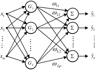
Generally, an RBFNN has a feed forward architecture, has three layers, input layer, hidden layer, and output layer. The basic structure of an RBFNN is shown in Figure 1. The output of the RBFNN can be expressed as follows
L i i c i ij ij L i i j w G t y 1 2 2 1 2 exp ) 1 (ˆ x x for j1, 2, , p (1)
where x( )t
x t1( ) x tm( )
T is the input vector, yˆ( )t y tˆ1( ) y tˆp( )T is theoutput vector of RBFNN, ij is the vector of the synaptic weights in the output layer, Gi
is the vector of the Gaussian function, denote the RBFNN activation function of the hidden
layer, xic and wi are the vector of the centers and widths in Gi, respectively, and L
is the number of neurons in the hidden layer.
1 G 2 G L G 1 x 2 x m x
yˆ1
yˆ2
yˆp
1 G 2 G L G 11 12
2 L Lp Figure 1. The structure of RBFNN.
In the training procedure, the initial values of parameters in (1) must be selected first. Then a training method is used to adjust these values iteratively to obtain their optimal combination. However, there is no way to systematically select the initial value of parameters. In the following section, an SVR is applied to perform this work.
3. AALA-SVR-RBFNN for STLF
3.1. SVR-based initial parameters estimation of RBFNN
( ) ( )
(xk ,yk ), k 1, 2, ,N.
In SVR, the Gaussian function is adopted as the kernel function [43, 44]. Therefore, approximating function can be rewritten as
bf
S V
N
l l
l
1 2 2 2 exp , x xl
x (2)
where NSV is the number of support vectors (SVs) and xl are SVs. Comparing (2) with
(1), NSV, l,
l,
l, and xl in (2) can be considered to be the L, i, ij, wi, andc i
x in (1), respectively. From the above derivation, the parameters of RBFNN in (1) can be
obtained through the above -SVR method.
3.2. AALA-based SVR-RBFNN
When computing the initial parameters of the SVR-RBFNN, one must establish a learning algorithm to get the optimal parameters of SVR-RBFNN. Based on time-varying learning rates, an AALA is used to train the SVR-RBFNN for conquering the drawbacks of low convergence and local minimum faced by the back-propagation learning method [44]. A cost function for the AALA is defined as
N k k jj e h h
N h 1 ) ( ) ( ); ( 1 )
( for j1, 2, ,p (3)
where
L i i c i k ij k j k j k j k j w y f y h e 1 2 2 ) ( ) ( ) ( ) ( ) ( 2 exp ) ( ˆ )( x x x (4)
h denotes the epoch number, e( )jk ( )h denotes the error between the jth desired output and
the jth output of RBFNN at epoch h for the kth input-output training data, (h) denotes
a deterministic annealing schedule acting like the cut-off point, and ( ) denotes a logistic
2 ) ( 1 ln 2 ; k j k j ee for j1, 2, , p (5)
The root mean square error (RMSE) is adopted to assess the performance of training RBFNN, given by
for (6)
According to the gradient-descent learning algorithms, the synaptic weights of ij, the
centers of xic, and the widths ofwi in Gaussian function are adjusted as
N k ij k j k j j ij j ij e e N 1 ) ( ) ( ; (7)
N k c i k j k j j p j c c i j c c i e e N 1 ) ( ) ( 1 ; x xx (8)
N k i k j k j j p j w i j w i w e e N w w 1 ) ( ) ( 1 ; (9)
) ( 1 ; ; 2 ) ( ) ( ) ( ) ( ) ( h e e e e e k j k j k j k j k j j (10)where
,
c, and
w are the learning rates for the synaptic weights ij, the centers, c i
x and the widths wi, respectively; and ( ) is usually called the influence function. In
ARLA, the annealing schedule (h) has the capability of progressive convergence [45, 46].
In annealing schedule, complex modifications to the sampling method have been proposed, which can use a higher learning rate to reduce the simulation cost [47-50]. Based on this concept, the non-uniform sampling rates of AALA are used to train BRFNN in this work. According to the relative deviation of the late epochs, the annealing schedule (h) can be
adjusted. The annealing schedule is updated as
2( ) 1 1 N k j k RMSE e N
( ) 1 m a x
h h h
for epoch h, (11)
, log 2 RMSE S (12) (13)
where is a constant, is the standard deviations, and is the average of RMSE
(6) for late epochs.
When the learning rates keep constant, choosing an appropriate learning rates
,
c,and
w is tedious; furthermore, several problems of getting stuck in a near-optimal solutionor slow convergence still exist. Therefore, an AALA is used to overcome the stagnation in the search for a global optimal solution. At the beginning of the learning procedure, a large learning rate is chosen in the search space. Once the algorithm converges progressively to the optimum, the evolution procedure is gradually tuned by a smaller learning rate in later epochs. Then, a nonlinear time-varying evolution concept is used in each iteration, in which
the learning rates
,
c, and
w have a high value max , nonlinearly decrease to minat the maximal number of epochs, respectively. The mathematical formula can be expressed as
min epoch(h) p (14)
pc
c min epoch(h) (15)
pw
w min epoch(h) (16)
max
min
(17) max 1 ) ( epoch h hepoch (18)
where epochmax is the maximal number of epochs and h is the present number of
21 1 , m i i
S RMSE RMSE
m
S RMSE
epochs. During the updated process, the performance of RBFNN can be improved using
suitable functions for the learning rates of
,
c, and
w. Furthermore, simultaneouslydetermining the optimal combination of p, pc, and pw in (14) to (16) is a
time-consuming work. An PSO algorithm with linearly time-varying acceleration coefficients will be used to obtain the optimal combination of (p, pc, pw).
3.3. Procedure of hybrid learning algorithm
The flowchart of AALA-SVR-RBFNN using PSO is illustrated in Figure 2. The solution of the average optimal value of (p, pc,pw) is determined using PSO through M times
independently. Then, the optimal structure of the proposed AALA-SVR-RBFNN is obtained.
4. Case studies
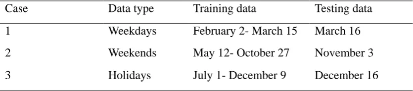
The 24-hour-ahead forecasting performance of the proposed AALA-SVR-RBFNN is verified on a real-word load dataset from Taiwan Power Company (TPC) in 2007. Three different patterns of load data, such as the working days (Monday through Friday), the weekends (Saturday), and holidays (Sunday and national holiday), are utilized to evaluate the effectiveness of the proposed algorithm. Table 1 lists the periods of the training and testing load data on TPC. The forecasting performance is also compared to those of DEKF-RBFNN [19], GRD-DEKF-RBFNN [19], SVR-DEKF-DEKF-RBFNN [19], and ARLA-SVR-DEKF-RBFNN. All our simulations are carried out in Matlab 2013a using a personal computer with Intel i3-6100 and 4G RAM, windows 7 as operating system.
The initial parameters in the simulations must be specified first. For the PSO parameters, the population size is set to be 40 and the maximal iteration number is set to be 200. Meanwhile, the number of generating different optimal sets of (p,pc, pw) is set to 10
) 10
real numbers in the interval [0.1,5]. Furthermore, the value of max is chosen to be 2.0 and
the value of min is chosen to be 0.05.
Table 1. The periods of the training and testing load data on TPC in 2007.
Case Data type Training data Testing data 1 Weekdays February 2- March 15 March 16
2 Weekends May 12- October 27 November 3
3 Holidays July 1- December 9 December 16
In order to evaluate the forecasting performance of the models, two forecast error measures, such as mean absolute percentage error (MAPE), and standard deviation of absolute percentage error (SDAPE), which are utilized for model evaluation, and their definitions are shown as follows:
100 1 1 ) ( ) ( ) (
N k k k k A F A N MAPE (19) 2 1 ) ( ) ( ) ( 100 1
N k k k k MAPE A F A NSDAPE (20)
where N is the number of forecast periods, A(k) is the actual value and F(k) is the forecast value. Moreover, the RMSE in (6) is employed to verify the performance of training RBFNN. Case 1: Load prediction of weekdays
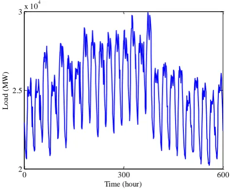
The training hourly actual load data are shown in Table 1 and Figure 3. After 1000 training
epochs, the initial parameters of RBFNN are determined by using SVR. The value of L in (1) is found to be 5 for parameters C1 and 0.05 in SVR. Meantime, the average optimal learning rate set of (p, pc,pw) is determined by PSO, which is found to be
Perform the adaptive annealing learning algorithm (AALA)
Initialize the population of position and velocity particles randomly; j = 0
Construct an initial structure of RBFNN using SVR; K = 0
Determine the local best and global best according to the fitness values of each population
Update the learning rate functions (14) through (16) using PSO method
Output the average optimal value of in (14) through (16)
Perform the adaptive annealing learning algorithm (AALA)
Determine the global best according to the fitness values of each population
Calculate the fitness values for each population using (6)
Calculate the fitness values for each population using (6)
Obtain the proposed AALA-SVR-RBFNN Yes
No M
K Yes
No
max
iter
j
1 j j
1
K
K
) , ,
(p pc pw
Figure 3. The training hourly actual load data in Case 1.
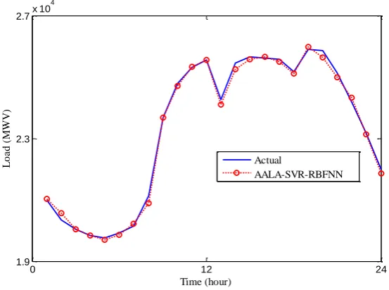
Figure 4. The forecasting results of the proposed AALA-SVR-RBFNN in Case 1.
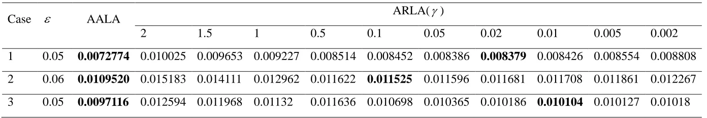
Table 2 lists the comparison results of RMSE in (6) between ARLA and AALA. In Table 2, it can be observed that AALA is superior to ARLA. After training, the proposed approach is evaluated on 24-hour-ahead load forecasting in March 16, 2007. From Figure 4, it can be observed that the predicted values of the proposed AALA-SVR-RBFNN are close to the actual values.
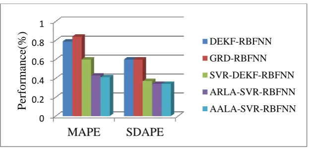
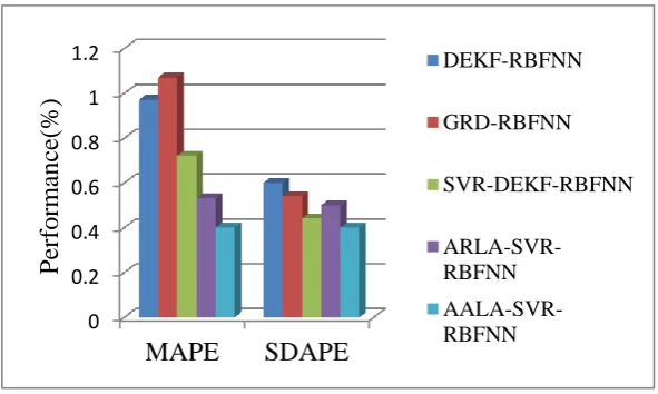
The comparisons of MAPE and SDAPE using the five prediction models are shown in
0 300 600
1.8 2.3 2.8x 10
4
Time (hour)
L
o
a
d
(
M
W
)
0 12 24
1.9 2.3 2.7x 10
4
Time (hour)
L
o
a
d
(
M
WV
)
Actual
Table 3 and Figure 5. From the comparisons, the value of MAPE of the proposed method is the smallest among the prediction approaches and has get the improvements of 48.10%, 51.19%, 31.67% and 4.65%the over DEKF-RBFNN [19], GRD-RBFNN [19], SVR-DEKF-RBFNN [19] and ARLA-SVR-SVR-DEKF-RBFNN, respectively. Moreover, the SDAPE value of the proposed AALA-SVR- RBFNN is 0.34%, less than those obtained by the four methods. Case2: Load prediction of weekends
The training hourly load data are shown in Table 1 and Figure 6. After 1000 training epochs,
the initial parameters of RBFNN are obtained by using SVR. The value of L in (1) is found to be 7 for parameters C 1 and 0.06 in SVR. Meantime, the average optimal learning rate set of (p, pc, pw) is determined by PSO, which is found to be (2.6007,
0.7976, 4.0978).
Figure 5. MAPE(%) and SDAPE(%) results for prediction methods in Case1.
0 0.2 0.4 0.6 0.8 1
MAPE SDAPE
Perform
ance(
%) DEKF-RBFNN
Table 2. Results of RMSE in (6) of the ARLA (0.002 2) and AALA after 1000 training epochs for three cases.
Case AALA ARLA( )
2 1.5 1 0.5 0.1 0.05 0.02 0.01 0.005 0.002
Table 3. MAPE(%) and SDAPE(%) results for prediction methods in Case1.
Method MAPE SDAPE
DEKF-RBFNN [19] 0.79 0.6
GRD-RBFNN [19] 0.84 0.6
SVR-DEKF-RBFNN [19] 0.6 0.37
ARLA-SVR-RBFNN 0.43 0.34
AALA-SVR-RBFNN 0.41 0.34
Figure 6. The training hourly actual load data in Case 2.
Table 2 shows the RSME in (6) ARLA and AALA. As seen from Table 2, the AALA can obtain an encouraging result than ARLA. After training, the proposed approach is evaluated on 24-hour-ahead load forecasting. Figure 7 shows that the predicted values of the proposed method are very close to the actual values.
0 300 600
2 2.5
3x 10
4
Time (hour)
L
o
a
d
(
M
W
Figure 7. The forecasting results of the proposed AALA-SVR-RBFNN) in Case 2.
The comparison results of MAPE andSDAPE using the five prediction models are shown in Table 4 and Figure 8. From the comparisons, the proposed AALA-SVR-RBFNN has the minimum value of MAPE. The proposed approach is 58.76%, 62.63%, 44.33%, and 24.53% better than DEKF-RBFNN [19], GRD-RBFNN [19], SVR-DEKF- RBFNN [19], and ARLA-SVR-RBFNN. Moreover, the value of SDAPE of the proposed algorithm is smaller than those of other four methods.
Figure 8. MAPE(%) and SDAPE(%) results for prediction methods in Case 2.
0 12 24
2 2.3 2.6x 10
4
Time (hour)
L
o
a
d
(
M
WV
)
Actual
AALA-SVR-RBFNN
0 0.2 0.4 0.6 0.8 1 1.2
MAPE SDAPE
Perform
ance(
%)
Table 4. MAPE(%) and SDAPE (%) results for prediction methods in Case 2.
Method MAPE SDAPE
DEKF-RBFNN [19] 0.97 0.6
GRD-RBFNN [19] 1.07 0.54
SVR-DEKF-RBFNN [19] 0.72 0.44
ARLA-SVR-RBFNN 0.53 0.5
AALA-SVR-RBFNN 0.4 0.4
Case3: Load prediction of Holidays
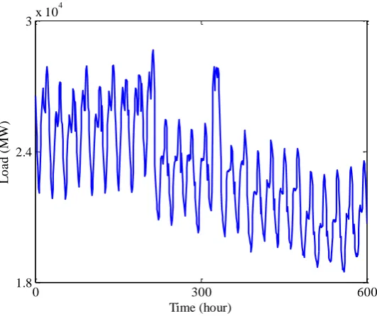
The training hourly load data are shown in Table 1 and Figure 9. After 1000 training epochs, the initial parameters of RBFNN are determined by using SVR. The value of L in (1) is found to be 11 for C1 and 0.05 in SVR. Meanwhile, the average optimal learning rate set of (p, pc, pw) is determined by PSO, which is found to be (1.9640, 0.8327,
4.9085).
Figure 9. The training hourly actual load data in Case 3.
0 300 600
1.8 2.4
3x 10
4
Time (hour)
L
o
a
d
(
M
W
Figure 10. The forecasting results of the proposed AALA-SVR-RBFNN in Case 3.
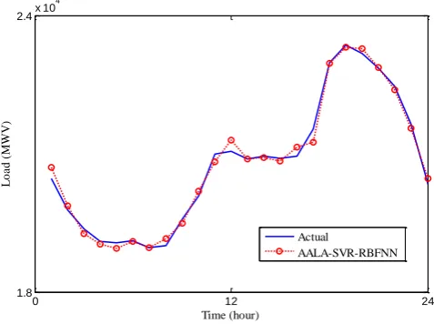
Table 2 illustrates the comparison results of RSME in (6) between ARLA and AALA. As seen from Table 2, the AALA can produce superior results than AALA. After training, the proposed approach is tested on 24-hour-ahead load forecasting. Figure 10 shows that the predicted values of the proposed AALA-SVR-RBFNN are quite close to the actual values.
Figure 11. MAPE(%) and SDAPE(%) results for prediction methods in Case3. Table 5. MAPE(%) and SDAPE(%) results for prediction methods in Case3.
Method MAPE SDAPE
DEKF-RBFNN [19] 0.89 0.52
GRD-RBFNN [19] 1.57 1.04
SVR-DEKF-RBFNN [19] 0.56 0.52
ARLA-SVR-RBFNN 0.62 0.51
AALA-SVR-RBFNN 0.49 0.38
0 12 24
1.8 2.4x 10
4
Time (hour)
L
o
a
d
(
M
WV
)
Actual
AALA-SVR-RBFNN
0 0.5 1 1.5 2
MAPE SDAPE
Perform
ance(
%)
The comparisons of MAPE and SDAPE using the five prediction models are shown in Table 5 and Figure 11. Comparing DEKF-RBFNN [19], GRD-RBFNN [19], SVR-DEKF-RBFNN [19], and ARLA-SVR-SVR-DEKF-RBFNN with the proposed AALA-SVR- SVR-DEKF-RBFNN, the error of MAPE is reduced by44.94%, 68.79%, 12.50%, and 20.97%, respectively. Moreover, the
SDAPE value of the proposed algorithm is 0.38%, smaller than those obtained by using the four approaches. These results verify that the superiority of the proposed AALA-SVR-RBFNN over other prediction methods.
5. Conclusions
In this paper, a reinforcement neural network of AALA-SVR-RBFNN is developed for predicting STLF accurately. An SVR method is first used to find the initial parameters of RBFNN. After initializations, the parameters of RBFNN are adjusted by using AALA to obtain an optimal combination. When performing the AALA, the optimal nonlinear learning rates are simultaneously determined by using PSO. Meantime, the stagnation of training RBFNN can be overcome during the adaptive annealing learning procedure. Once the optimal RBFNN is established, the 24-hour-ahead load forecasting is to be performed. Three different patterns of load are considered. Simulation results indicate that the proposed AALA-SVR-RBFNN can yield excellent forecasting results over DEKF-RBFNN, GRD-RBFNN, SVR-DEKF- GRD-RBFNN, and ARLA-SVR-RBFNN.
Acknowledgment
This work was supported in part by the National Science Council, Taiwan, R.O.C., under grants MOST 105-2221-E-252-002.
References
Short Term Electrical Load Forecasting.” Energies, vol.6, (2013), pp.2130-2148. [2] Hernandez L; Baladrón C; Aguiar J M, et al. “Short-Term Load Forecasting for
Microgrids Based on Artificial Neural Networks.” Energies, vol.6, (2013),
pp.1385-1408.
[3] Amjady N; Keynia F. “A New Neural Network Approach to Short Term Load Forecasting of Electrical Power Systems.” Energies, vol.4, (2011), pp.488-50.
[4] Wang J; Jiang H; Wu Y, et al. “Forecasting solar radiation using an optimized hybrid model by Cuckoo Search algorithm.” Energy, vol.81, (2015), pp.627–644.
[5] Shahidehpour M; Yamin H; Li Z. “Market operations in electric power systems: forecasting, scheduling, and risk management.” John Wiley & Sons, (2002).
[6] Christiaanse W R. “Short term load forecasting using general exponential smoothing.” IEEE Transactions on Power Apparatus and Systems, PAS-90, (1971), pp.900-911. [7] Dudek G. “Pattern-based local linear regression models for short-term load forecasting.”
Electric Power Systems Research, vol.130, (2016), pp.139-147.
[8] Darbellay G A; Slama M. “Forecasting the short-term demand for electricity.” International Journal of Forecasting, vol.16, (2000), pp.71-83.
[9] Zheng T; Girgis A A; Makram E B. “A hybrid wavelet-Kalman filter method for load forecasting.”Electric Power Systems Research, vol.54, (2000), pp.11-17.
[10] Gouthamkumar N; Sharma V; Naresh R. “Non-dominated sorting disruption-based gravitational search algorithm with mutation scheme for multi-objective short-term hydrothermal scheduling.” Electric Power Components and Systems, vol.44, (2016), pp.990-1004.
[11] Mori H; Kobayashi H. “Optimal fuzzy inference for short-term load forecasting.” IEEE Transactions on Power Systems, vol.11, (1996), pp.390-396.
pp.425-433.
[13] Hong W C. “Electric load forecasting by support vector model.” Applied Mathematical Modelling, vol.33, (2009), pp.2444-2454.
[14] Niu M F; Sun S L; Wu J, et al. “An innovative integrated model using the singular spectrum analysis and nonlinear multi-layer perceptron network optimized by hybrid intelligent algorithm for short-term load forecasting.” Applied Mathematical Modelling, vol.40, (2016), pp.4079-4093.
[15] Bashir Z A; El-Hawary M E. “Applying Wavelets to Short-Term Load Forecasting Using PSO-Based Neural Networks.” IEEE Transactions on Power Systems, vol. 24, (2009), pp.20-27.
[16] Panapakidis I P. “Application of hybrid computational intelligence models in short-term bus load forecasting.” Expert Systems with Applications, vol.54, (2016), pp.105-120. [17] Ceperic E; Ceperic V; Baric A. “A strategy for short-term load forecasting by support
vector regression machines.” IEEE Transactions on Power Systems, vol. 28, (2013), pp.4356-4364.
[18] Li S; Wang P; Goel L. “Short-term load forecasting by wavelet transform and evolutionary extreme learning machine,” Electric Power Systems Research, vol. 122, pp. 96-103, 2015.
[19] Ko C N; Lee C M. “Short-term load forecasting using SVR (support vector regression)-based radial basis function neural network with dual extended Kalman filter.” Energy, vol.49 (2013) , pp.413-422.
[20] Lin Z; Zhang D; Gao L, et al. “Using an adaptive self-tuning approach to forecast power loads.” Neurocomputing, vol.71, (2008), pp.559-563.
[22] Attoh-Okine N O. “Analysis of learning rate and momentum term in backpropagation neural network algorithm trained to predict pavement performance.” Advances in Engineering Software, vol. 30, (1999), pp.291-302.
[23] Nied A; Seleme Jr SI; Parma G G, et al. “On-line neural training algorithm with sliding mode control and adaptive learning rate.” Neurocomputing, vol.70, (2007), pp.2687-2691.
[24] Hsieh S T; Sun T Y; Lin C L, et al. “Effective learning rate adjustment of blind source separation based on an improved particle swarm optimizer.” IEEE Transactions on Evolutionary Computation, vol.12, (2008), pp.242-251.
[25] Li Y; Fu Y; Li H, et al. “ The improved training algorithm of back propagation neural network with self-adaptive learning rate.” in Processing of International Conference on Computational Intelligence and Natural Computing (CINC 2009), Wuhan, China, (2009), pp.73-76.
[26] Lin C L; Hsieh S T; Sun T Y. “PSO-based learning rate adjustment for blind source separation.” in Proceedings of the International Symposium on Intelligent Signal Processing and Communication System (ISPACS 2005), Hong Kong, (2005), pp. 181-184.
[27] Song G J; Zhang J L; Sun Z L. “The research of dynamic change learning rate strategy in BP neural network and application in network intrusion detection.” in Proceedings of the 3rd International Conference on Innovative Computing Information and Control (ICICIC 2008), Liaoning China. (2008), pp.513-513.
[28] Fernandez-Navarro F; Hervas-Martinez C; Ruiz R, et al. “Evolutionary generalized radial basis function neural networks for improving prediction accuracy in gene classification using feature selection.” Applied Soft Computing, vol.12, (2010), pp.1787-1800.
algorithm for growing and pruning RBF (GAP-RBF) networks.” IEEE Transactions on Systems, Man, and Cybernetics - Part B: Cybernetics, vol.34, (2004), pp.2284-2292. [30] Kokshenev I; Braga A P. “A multi-objective approach to RBF network learning.”
Neurocomputing, vol.71, (2008), pp.1203-1209.
[31] Kokshenev I; Braga A P. “An efficient multi-objective learning algorithm for RBF neural network.” Neurocomputing, vol.73, (2010), pp.2799-2808.
[32] Kumar R; Ganguli R; Omkar S N. “Rotorcraft parameter estimation using radial basis function neural network.” Applied Mathematics and Computation, vol.216, (2010), pp.584-597.
[33] Zhang M L; Wang Z J. “MIMLRBF: RBF neural networks for instance multi-label learning.” Neurocomputing, vol.72, (2009), pp.3951-3956.
[34] Asirvadam V S; McLoone S F; Irwin G W. “Computationally efficient sequential learning algorithms for direct link resource-allocating networks.” Neurocomputing, vol.69, (2005), pp.142-157.
[35] Huynh H T; Won Y. “Regularized online sequential learning algorithm for single-hidden layer feedforward neural networks.” Pattern Recognition Letters, vol. 32, (2011), pp.1930-1935.
[36] Liang N Y; Huang G B; Saratchandran P, et al. “A fast and accurate online sequential learning algorithm for feedforward networks.” IEEE Transactions on Neural Networks, vol.17, (2006), pp.1411-1423.
[37] Lu Y; Sundararajan N; Saratchandran P. “Performance evaluation of a sequential minimal radial basis function (RBF) neural network learning algorithm.” IEEE Transactions on Neural Networks, vol.9, (1998), pp.308-318.
allocation network classifier.” Neurocomputing, vol.73, (20120), pp. 3012-3019. [40] Suresh S; Savitha R; Sundararajan N. “Sequential learning algorithm for
complex-valued self-regulating resource allocation network-CSRAN,” IEEE Transactions on Neural Networks, vol.22, (2011), pp.1061-1072.
[41] Zhou Z J; Hu C H; Yang J B, at al. “A sequential learning algorithm for online constructing belief-rule-based systems.” Expert Systems with Applications, vol.37, (2010), pp.1790-1799.
[42] Ko C N. “Reinforcement radial basis function neural networks with an adaptive annealing learning algorithm.” Applied Mathematical Modelling, vol.221, (2013), pp.503-513.
[43] Vapnik V. “The nature of statistic learning theory.” New York: Springer-Verlag, (1995). [44] Chuang C C; Jeng J T; Lin P T. “Annealing robust radial basis function networks for
function approximation with outliers,” Neurocomputing, vol.56, (2004), pp. 123-139. [45] Fu Y Y; Wu C J; Jeng J T, et al. “Identification of MIMO systems using radial basis
function networks with hybrid learning algorithm.” Applied Mathematics and Computation, vol.213, (2009), pp.184-196.
[46] Chuang C C; Su S F; Hsiao C C. “The annealing robust backpropagation (BP) learning algorithm.” IEEE Transactions on Neural Networks, vol.11, (2000), pp. 1067-1077. [47] Alrefaei M H; Diabat A H. “A simulated annealing technique for multi-objective
simulation optimization.” Applied Mathematics and Computation, vol. 215, (2009), pp. 3029-3035.
[48] Ingber L. “Very fast simulated re-annealing.” Mathematical and Computer Modelling, vol.12, (1989), pp.967-983.
[50] Shieh H L; Kuo C C; Chiang C M. “Modified particle swarm optimization algorithm with simulated annealing behavior and its numerical verification.” Applied Mathematics and Computation, vol.218, (2011), pp.4365-4383.