Multi-Modal Perception for Selective Rendering
Carlo Harvey, Kurt Debattista, Thomas Bashford-Rogers and Alan Chalmers
WMG, University of Warwick, UK.
Abstract
A major challenge in generating high-fidelity virtual environments (VEs) is to be able to provide realism at in-teractive rates. The high-fidelity simulation of light and sound is still unachievable in real-time as such physical accuracy is very computationally demanding. Only recently has visual perception been used in high-fidelity ren-dering to improve performance by a series of novel exploitations; to render parts of the scene that are not currently being attended to by the viewer at a much lower quality without the difference being perceived. This paper investi-gates the effect spatialised directional sound has on the visual attention of a user towards rendered images. These perceptual artefacts are utilised in selective rendering pipelines via the use of multi-modal maps. The multi-modal maps are tested through psychophysical experiments to examine their applicability to selective rendering algo-rithms, with a series of fixed cost rendering functions, and are found to perform significantly better than only using image saliency maps that are naively applied to multi-modal virtual environments.
Categories and Subject Descriptors (according to ACM CCS): I.3.3 [Computer Graphics]: Picture/Image Generation—Viewing Algorithms I.4.8 [Computer Graphics]: Image Processing and Computer Vision—Scene Analysis - Object Recognition I.4.8 [Computer Graphics]: Image Processing and Computer Vision—Scene Anal-ysis - Tracking
Keywords:Multi-Modal, Cross-Modal, Saliency, Sound, Graphics, Selective Rendering
1. Introduction
A major research challenge of Virtual Environments (VEs) is to accurately simulate a real world environment. This is motivated by the increasing use of VEs in a wide range of applications such as concert hall and architectural de-sign [Dal,Nay93] and immersive video games [MBT∗07,
RLC∗07,GBW∗09]. Multi-modal VEs aim to deliver more sensory information than from a sole domain and yield an increased sense of immersion over single modality environ-ments [DM95]. Furthermore, such multi-modal VEs can aid object recognition and placement; identification and local-isation; and generating conclusions pertaining to the scale and shape of the environment [Bla97].
Limitations of the human sensory system have been used in order to improve the performance of perceptually-based rendering systems. Examples of this used to decrease the auditory [TGD04,MBT∗07] or visual [CCL02,RFWB07,
RBF08] rendering complexity with little or no perceivable quality difference to a user have been implemented and ver-ified. Moreover, it has been shown that it is possible to in-crease the perceptual quality of a stimulus in one
modal-ity by directing gaze due to the introduction of another modality [MDCT05a]. This can be used for improving the perception of a material’s quality [BSVDD10], Level-of-Detail (LOD) selection [GBW∗09] or for increasing the spatial [MDCT05a,HHT∗11] and temporal [MDCT05b,
HHT∗11,HDAC10] quality of visuals by coupling them with corresponding auditory stimuli.
spatial localisation of objects [DS98]. In this paper we pro-pose a general algorithm to concatenate sound saliency with visual saliency in the spatio-visual domain. In particular, this paper considers the effect of directional sound on a user’s visual attention towards rendered images. Based on a sound transport simulation, multi-modal maps are derived. These are used to reduce render times while maintaining perceptual equality. This is validated in a further user study. Specifically we make the following contributions:
• Construction of a sound map which encodes directional sound saliency information. These are produced through a sound simulation based on tracing phonons [BDM∗05].
• Utilising the sound maps to represent saliency of a direc-tional sound signal and using density estimation to con-struct a saliency map for the spatial domain.
• Combination of the traditional visual saliency map with the directional sound saliency map into a multi-modal saliency map. This is used to reduce rendering time in this paper. The technique could be more broadly applied to any audio-visual interface requiring a degrade function, such as compression of video.
• A user study which validates the use of the multi-modal maps to reduce rendering time, but maintaining similar perceptual quality to reference images computed at higher sampling rates.
2. Background and Related Work 2.1. Images
Saliency models have been used previously in computer graphics, and more so in computer vision applications. Yee et al. [Yee00,YPG01] adapted Itti and Koch’s [IKN98] model of visual saliency in order to speed up the render-ing process. For each frame a spatiotemporal error tolerance map [Dal98] was created based on velocity dependant con-trast sensitivity, and a saliency map [IKN98]. The two maps were combined to create a new map, termedaleph map. The aleph map was used to determine where computational re-sources were to be directed in screen space.
Marmitt et al. [MD02] examined how Itti and Koch’s [IKN98] model performed when predicting vi-sually salient features in virtual scenes. The model had been shown to perform accurately on real imagery [PS00], however the analysis showed that the correlation between human saccades and model predicted saccades was quite low. Marmitt et al. [MD02] hypothesised that the lack of correspondence between real and predicted views occurred due to the absence of a memory module in the artificial model. The human brain has temporal memory and remembers what it has seen.
More recent work by Koulieriset al.[KDCM14] showed a method to extend a recent saliency model, incorporating ef-fects such as object context, uniqueness of objects and tem-porality. This allowed an attention based level-of-detail man-ager to constrain material quality in presented images whilst
maintaining frame rate. The benefit of this technique in a proof of concept was to incorporate parallax occlusion map-ping on a mobile device. For a full overview on perception in graphics please see [MMG11].
2.2. Sound
The computational bottlenecks in sound rendering can be grouped into two broad types: the cost of acoustic spatial-isation and the cost per sound source. The processing of complex sound scenes is composed of spatialisation and per source information. This can take advantage of perceptually-based optimisations in order to reduce both the necessary computer resources and the amount of audio data to be stored and processed. The MPEG I Layer 3 (mp3) stan-dard [PS00] is one such example of this which exploits Per-ceptual Audio Coding (PAC), where prior work on auditory masking [Moo97] had been successfully utilised. This is im-plicitly used together with masking to discard information of audio content deemed perceptually irrelevant from the origi-nal sound. The missing audio content is not perceived in the resultant sound.
The auditory saliency map presented by Kayser et al.[KPLL05] has been used to predict the parts of a sound source that will attract human attention, so that more re-sources in the acoustic rendering process could be assigned for their computation.
This method was adapted by Moecket al.[MBT∗07] for acoustic rendering by integrating saliency values over fre-quency subbands. They suggested using auditory saliency as a heuristic for the clustering stage of multiple audio sources. Recent work on the synthesis of sound, showed that com-bining the instantaneous energy of the emitted signal and attenuation is also a good criteria [GLT05,Tsi05].
The presence of many sensory stimuli, including sound, may influence the amount of cognitive resources available to a viewer to perform a visual task, this is termed as themodality appropriateness hypothesis[WW80]. Research has investigated the influence of auditory cues on visual attention and visual cues on audition. Mastoropoulou et al.[MDCT05a,MDCT05b] showed that a selective render-ing technique for Sound Emittrender-ing Objects (SEO) can be used to render animations, and can decrease the rendering time required. Considering the angular sensitivity of the Human Visual System (HVS) and inattentional blindness, the visual region that contained the SEO was rendered in high qual-ity at an appropriate angle, whilst low qualqual-ity visuals were displayed for the rest of the scene and the viewer failed to notice the quality difference.
the perceived temporal smoothness of graphics, while con-gruent audio has no significant effect on the perceived qual-ity threshold. Grelaudet al.[GBW∗09] developed a model to detect when many instances of vibratory and contact syn-thesis were occurring and to fluctuate resources accordingly from the visual domain to the auditory domain dynamically. As a result, visuals were poorer when many objects col-lided and audio was deemed more important. This directly attempted to exploit themodality appropriateness hypothe-sis. However, even though the result showed the technique worked and perception was unaltered, no empirical tech-nique was used and the variability of resources was user de-fined and for a specific task. A generic model for bi-modal scenarios (auditory-visual interaction) has yet to be consid-ered.
3. Modal Map Generation
A novel temporal acoustic algorithm for spatial visual saliency prediction is presented in this section. The algo-rithm is based upon sound-level-detection on the image plane modulated by the auditory salience feature vector of an asynchronous acoustic stimulus. Blended with conventional visual saliency predictors this enables spatial heuristics to guide sample count for rendering to be employed. In Section
4we show that this provides better perceptual responses than previous image synthesis sampling strategies.
3.1. Algorithm: Intensity Map
A two step approach to generate the directional inten-sity of the sound wave on the image plane is used. The first step utilises the algorithm employed by the sonel and phonon mapping techniques for sound rendering [KJM04,
BDM∗05]. This is a particle tracing based method where starting points and directions of paths are generated on the sound source and propagate around the scene. Information at each hit point is stored and used in a second stage to re-construct the sound at the listener position.
Initially, the sound source is approximated by a set of frequencies, and for each sound-carrying particle one fre-quency is sampled. Then the starting point and direction of the sound particle is selected according to the emission dis-tribution of the sound source. This sound particle is then traced into the scene, and at each intersection (including the initial point on the sound source) a set of information is stored. This consists of sound intensity values attributed to each hit point: pressure (P), frequency (F), incoming direction (ωi) and world space position (x0). These points are stored in a KD-Tree for fast searching in the second step. This could also be implemented through a splatting approach, akin to Progressive Photon Mapping [HOJ08]. Whilst splatting is fast, our approach avoids heuristically set-ting a splat radius, which leads to a smooth intensity map regardless of the number of sound particles traced. Informa-tion such as world space posiInforma-tion is used from the KD-Tree later when generating the binaural audio as the sound paths
need to be connected to the Head Related Impulse Response (HRIR) for evaluation. The reflection type at the intersection is then sampled, the intensity of the sound particle is appro-priately modulated, and the tracing continues. This process continues until the tracing process is terminated stochasti-cally via Russian Roulette. This process is shown in Algo-rithm1.
Algorithm 1:Sound Particle Tracing KD-Tree kd
foreach sound particledo
Sample frequencyF
Sample sound source emission
Store sound particle on sound source in kd Generate ray starting at sound source
whilePath is not terminateddo
Store sound particle at intersection in kd Sample surface reflection and generate ray Apply Russian Roulette
end while end for
The second step generates the auditory intensity map through density estimation using the previously stored sound particles. This is a view-dependent map which encodes the intensity of the sound at points visible in the scene in the view direction. A ray is generated for each pixel using jit-tered sampling, and density estimation is performed at each primary hit pointxusing a balloon estimator for a KNN-search. This expands an initial search radius in world space untilNsound particles are located. This process is accel-erated using the KD-Tree which stores the sound particles. Once theN nearest sound particles to the primary ray hit point are found, a density estimate is performed according to the following equation:
So= 1 πr2
N
∑
i=1
P(i)f r(x0(i),ωi(i),ωo,F(i)) (1)
whereSois the pressure at the primary hit pointx,ris the radius from the KNN-search,P(i)is the pressure associated with thei’th nearest sound particle,f r(x0(i),ωi(i),ωo,F(i))
is the frequency dependent surface auditory reflectance func-tion (see Siltanen et al. [SLKS07]) at pointx0parameterised by thei’th incoming sound particle directionωi(i), the di-rection to the listenerωo and frequency Fi. This function encodes how sound of a certain frequencyF reflects off a surface. The valueN is a user defined value (we use 50). This step is shown in Algorithm2.
Algorithm 2:Auditory Intensity Map Generation
foreach pixelpdo
Sample pixel and generate ray Calculate hitpointx
FindNnearest sound particles Calculate pressure atx(Equation1) Store pressure in map atp
end for
Sound Particles Intensity Map
Lounge
Kitchen
Restaurant
Figure 1: Sound Particles Visualisation and Intensity Maps. The Sound Particles are shown as points and are coloured by stored pressure, red to blue, 1 to 0. The sound sources are denoted by an "S" character in the images. The lounge sound is a phone ringing, the kitchen sound a microwave starting up and running and the restaurant sound is a sample of music emanating from the speakers.
3.2. Temporal Map
Hearing is substantially weaker than vision in spatially re-lated tasks. However, the temporal resolution of the Human Auditory System (HAS) is higher than the visual temporal resolution. According to Fujisaki et al. it is 89.3Hz [FN05]. In order to make the auditory intensity map applicable tem-porally to the spatial domain it is necessary to weight the importance of the generated spatial sound intensity map. The work in auditory saliency maps can do this by predicting im-portant regions of the acoustic profile into temporal feature vectors. These feature vectors sit as a weight between us-ing the sound intensity maps and visual saliency maps in a perceptual selective temporal renderer.
In addition, the application of a spline introduces the weight in advance of the predicted onset and thus allows the selective renderer pipeline to not be reactive to attentional
models but to be proactive and sample an area in advance of predicted attention towards that area. More information on this spline can be found in Section4.3.4.
Fusion for audio-visual inputs can be performed at two distinct levels:low-level, at the extracted saliency; or high-level, at the original feature vector level. Given a video stream, audio-visual salience would be construed as a tem-poral sequence of audio-visual saliency values. This would have each value represent a measure of importance of the multi sensory stream at every framem. This may result in some form of fusion of the two features, which may be non-linear, have some form of memory or vary with time. For example, for the purposes of the experiments presented in Section4, this paper proceeds with a linear and memoryless schema for this audio-visual fusion:
S[m] =wA·SA[m] +wV·SV[m] (2)
where the weightswA and wV assigned to the fusion can be perceptually guided based upon a high level load balanc-ing framework. However, in the case of the experiment pre-sented in Section4these are assigned values:wA=FV[m] andwV =1−FV[m]whereFV[m]is the sound saliency fea-ture vector trace for the relevant audio sample corresponding to framem.SAandSV are the selective guidance mechanism for the image plane for the different modalities, audio and vi-sual respectively. This acts as a temporal slider between the standard visual saliency map and theauditory intensity map based upon the salient features of the acoustic information.
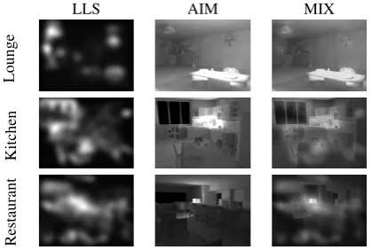
Figure2shows the original visual saliency, the sound in-tensity map, and a weighted combination for frame number m=180, time = 3s. This is shown for the Lounge, Kitchen and Restaurant scenes with the respective value ofFV[m] for the relevant audio on a scene by scene basis guiding the weighting.
LLS AIM MIX
Lounge
Kitchen
Restaurant
4. Psychophysical Experimental Layout and Procedure
The psychophysical experiment outlined in this section in-tends to validate two frequently used selective rendering op-erators against the algorithm reported in Section3.1and also a non-temporal intensity-only version of this.
4.1. Method
Four rendering strategies are used to evaluate the two meth-ods presented in the previous section and compare with more traditional methods:Uniform(Uni), each pixel is sampled uniformly;Visual Saliency(Sal), each pixel is sampled based on the visual attention prediction map;Sound Intensity Map (SoSal), each pixel is weighted based upon the auditory saliency trace and the intensity map from acoustic simula-tion only; and,Temporal Map(Mix), each pixel is sampled by a weighted combination of the visual saliency map and the temporal auditory saliency trace weighted by the direc-tional intensity acoustic simulation.
Pairwise comparisons amongst all the renderings for three scenes were used to judge the proposed methods. Pairwise comparisons were chosen as there were not that many tech-niques to compare against so a comparison of all methods against each other was feasible within a reasonable time. Participants were asked to always choose one of the two pairs (forced choice).
The experiment used 18 image pairs, six comparisons for each of three scenes presented in Section4.3.1. The condi-tions investigate the effect of various maps against one an-other in a pairwise performance test. The rendering strate-gies are governed, not by the algorithm, but by the pixel sampling strategy and the render function cost.
4.2. Participants
A total of 28 participants took part in this experiment, 21 males and 7 females. Participants reported no hearing dif-ficulties and normal or corrected-to-normal vision. The age range of participants was between 21 and 42, with an aver-age aver-age of 27. Each participant was presented with all of the scenes, thus looking at a total oft(t−21)×3= 4(23)×3=18 image pairs.
4.3. Materials
The participant sat on a chair, with the backrest of the chair 115 cm from the display. Binaural headphones were used for audio delivery and the monitor used was a 37" LCD panel display. The resolution of the LCD panel was 1024×768 with a refresh rate of 60 Hz and images displayed corre-sponded to this resolution so no up or down scaling was nec-essary and the images were displayed natively. The 2 chan-nel audio streams encoded the attenuation and delays of the HRIR for every sound contribution path reaching the user in the simulation. The convolved sound was represented as a two channel lossless 24-bit.wavfile.
A significant number of materials and parameters have been used for the user study so they are discussed in detail in the following subsections.
4.3.1. Scenes
Three different scenes of varying complexity were used, each with a static camera. Figure4demonstrates renders (and saliency maps) of the three scenes termed: Lounge, Kitchen and Restaurant. The sound sources used in each of these scenes were congruent to the scene and were represen-tative of an object in the scene. In the Lounge scene there was a phone ringing, in the Kitchen scene the microwave was turned on and, finally, in the Restaurant there was some music playing from the speakers. Each of the sounds was spatialised for that point and the listener was positioned at the same position as the camera.
4.3.1.1. Render Cost Function: In a selective rendering pipeline given a map as a heuristic to weight the sampling strategy; a cost to compute an image in terms of the degree of sampling used can be given as:
V=
w
∑
x=0 h
∑
y=0
smin+ ((smax−smin)·sal(x,y)) (3)
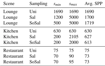
whereV is the number of samples required to compute an image,sminis the minimum number of samples used to cal-culate radiance through a pixel,smaxis the most number of samples used to calculate this,sal(x,y)is the weighting co-efficient for a specific pixel in image space, andxandyare pixel coordinates.
Scene Sampling smin smax Avg. SPP
Lounge Uni 1690 1690 1690
Lounge Sal 1200 5000 1700
Lounge SoSal 500 5000 1719
Kitchen Uni 630 630 630
Kitchen Sal 200 2105 627
Kitchen SoSal 200 2000 613
Restaurant Uni 75 75 75
Restaurant Sal 70 90 73
Restaurant SoSal 70 95 73
Table 1: Render Cost Function Across Scenes. Avg. SPP (Samples per pixel) is the average number of samples used to generate an image, dictating complexity.
To investigate the perceptual difference between two se-lective rendering strategies it is necessary to control this ren-der cost function so that, given a number of samples to gen-erate each image,V, an optimisation process starts to vary sminandsmax such that(S≈V)±f where f is some user defined control of sufficient leeway to compensate for the fact thatsminandsmaxare restricted to integers in the opti-misation process andSis the actual number of samples used in the generation of the image.
shows the varioussmin,smaxfor the various sampling meth-ods used.
The Visual Difference Predictor (VDP) [Dal93] results of comparisons between the three sampling strategies are pre-sented in Table2and shown in Figure3. The VDP results show there are distinct differences between the selectively rendered images for the same computational costs; effec-tively indicating that without sound there are clear differ-ences between the methods.
Scene Uni vs. SoSal Uni vs. Ref SoSal vs. Ref
Lounge 28.8546% 45.8543 % 13.8315%
Restaurant 7.17% 75.6775% 80.0777%
Kitchen 8.4064% 63.4815% 63.0377%
Table 2: Selective Render VDP Analysis at P>75%
SoSal vs. Uni Ref vs. SoSal Ref vs. Uni
Lounge
Kitchen
Restaurant
Figure 3: Selective Render VDP Image Comparisons. From top to bottom by row; Lounge, Kitchen and Restaurant scenes respectively. This probability of detection map dis-plays how likely a difference between two images is notice-able. Red denotes high probability, green - low probability.
4.3.2. Vision
Visual saliency predictor maps are computed using Itti et al’s method [IKN98]. The saliency maps are shown in Figure4. This step used the reference uniform path traced image as the input to the saliency generation. However a GPU snap-shot of the scene could just as easily be used in a real time implementation of this pipeline, as suggested by Longhurst et al. [LDC06] and by Yeeet al.[YPG01].
4.3.3. Audio
The binaural format was chosen to reproduce acoustic spa-tialisation features within the multi-modal VR environment. The pipeline calculates the Room Impulse Response (RIR) in the environment for a particular sound source location and listener position. This RIR encodes how the sound paths travel from the source to the listener in the environment.
Low Level Saliency Path Traced Render
Lounge
Kitchen
Restaurant
Figure 4: Low level Saliency Maps and the Path Traced Ren-ders of the three scenes. The audio reproduced in each room; Lounge - Phone, Kitchen - Microwave, Restaurant - Speaker playing music.
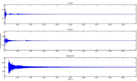
To convert this to binaural, a modelled Head-Related Trans-fer Function (HRTF) was implemented using the structural models of the Aural Time Difference (ITD) and Inter-Aural Level Difference (ILD) equations. This was done per Npaths in the acoustic simulation for each azimuth and ele-vation to the listener position. These delays and attenuations are convolved with the RIR to provide a binaurally encoded impulse response. Figure5shows the RIRs from the scenes used.
Simulations were performed on monaural anechoic sound and using the pipeline described above, rendered to encode spatial features of the presented environments: phones in the lounge, microwave in the kitchen and speaker playing mu-sic in the restaurant. In order to generate the RIRs, accu-rate material absorption coefficients had to be used in the environment to accurately encode the frequency responses of different material absorption rates. Common materialαf values per frequency were used appropriately throughout the scenes on correspondent surfaces, after [Sur12].
4.3.4. Auditory Saliency: Feature Vector Curves:
0 0.01 0.02 0.03 0.04 0.05 0.06 0.07 0.08 0.09 -1
-0.5 0 0.5 1
Lounge
0 0.01 0.02 0.03 0.04 0.05 0.06 0.07 0.08 0.09 -1
-0.5 0 0.5 1
N
o
rma
lize
d
a
mp
lit
u
d
e
Kitchen
0 0.01 0.02 0.03 0.04 0.05 0.06 0.07 0.08 0.09 -1
-0.5 0 0.5 1
Time, s Restaurant
Figure 5: Scene Room Impulse Responses; (top) Lounge, (middle) Kitchen, (bottom) Restaurant. A room impulse response is the response of an environment to an input signal, in this case an approximation to an ideal Dirac Delta function.
of an audio saliency curve is a weighted linear combina-tion of the normalised features. A perceptually motivated ap-proach is a non-linear fusion technique, based on time vary-ing weights. Temporal variation information is extracted by the onset and offset portions, while spectral change is cal-culated from the intermediate sustain periods. Energy mea-surement has previously been used to detect speech event boundaries [KPLL05] and as such is used as an index to an event of a transitional point.
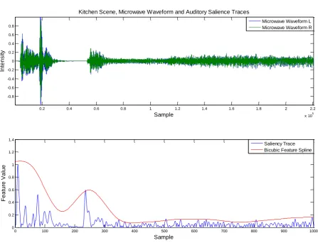
For use in the selective rendering pipeline the values from the saliency trace need to be absolute values and then nor-malised so the trace lies in the rangex∈0,1:x=||xˆ||. Fitting a spline to this in order to smooth map transition states helps to mitigate flickering as weights are altered. Other metrics may be chosen for this process of regularisation, such as a solid blur. Whilst the HVS supports an element of flicker fu-sion at the rate of 26Hz [HS36], temporal discrepancies are still picked up. Due to thetemporal sensitivityof the HAS the important parts of the vector are the most salient, and thus highest values. The saliency trace,x, was processed into ten bins of max values. These values were used as derivatives for a 1-D bicubic spline interpolation. The bicubic interpo-lation problem consists of determining the 1000 coefficients ai jto upsample the vector back to the appropriate size. Fig-ure6shows the original absolute normalised saliency feature vectors (trace), ˆxand the bicubic spline fit version for the
mi-crowave sound in the Kitchen scene. This process is shown for a 1-D spline fitp(x,y)whereai jare constants:
p(x,y) = 1000
∑
i=1 1
∑
j=1
ai jxiyj (4)
4.3.5. Temporal Modal Map
In the absence of animations and just single image exposure it was possible to blend the Sal render and the SoSal render temporally guided by the relevant feature vectors for Mix. A timer kept track of which feature value in the vector was appropriate for the current time. A shader read this from a text file of precomputed feature values and two textures were blended to create the final temporal composite.
4.4. Procedure
0.2 0.4 0.6 0.8 1 1.2 1.4 1.6 1.8 2 2.2
x 105
-0.8 -0.6 -0.4 -0.2 0 0.2 0.4 0.6 0.8
Sample
In
te
n
s
it
y
Kitchen Scene, Microwave Waveform and Auditory Salience Traces
0 100 200 300 400 500 600 700 800 900 1000
0 0.2 0.4 0.6 0.8 1 1.2 1.4
Sample
F
e
a
tu
re
V
a
lu
e
Microwave Waveform L Microwave Waveform R
Saliency Trace Bicubic Feature Spline
Figure 6: Microwave Waveform and Saliency Traces
were briefed prior to the experiment in order to gain a clear understanding of their task.
Each participant was assigned the 18 image sets in ran-dom order and the A or B image was ranran-domised within that image (slide) set. Participants were presented videos in the order A→G→B with a decision slide that waited for an in-put:“which video A or B is closest, in your opinion, to slide G?”, where G is the gold standard reference, enforcing two alternative forced choice assessment. This ordering was cho-sen as opposed to side-by-side because the sound would be mismatched spatially if the participant had to look between screens. A→G→B→G heuristic could have been chosen but repeated exposure to the same material could introduce more bias and was deemed less appropriate. Image videos were presented asynchronously with the relevant modality for a total of five seconds each. Buffer slides, providing a visual cue (displaying A or B) as to the current video to be shown were presented for two seconds before the advent of the re-spective video. The decision slide halted the experiment and waited indefinitely for a response on the pairwise compari-son (input A or B on the keyboard). Spatial sound congruent
to the object in the scene was delivered to the participant for the full duration of the relevant videos.
5. Results & Analysis
This section presents the results of the experiment. The overall similarity results for the 3 scenes are shown in Tables3,4and5. The paired comparison data is provided in Table7and coloured rings highlight that no significant dif-ference resulted in between the selective rendering strategies on a per scene and/or overall basis.
5.1. Statistical Analysis
The null hypothesis is given asH00, that all conditions are equal under testing (H00:πi= 12). The alternative being that not all the conditionsπiare equal.pi jis the number of times that an imageiis preferred to imagejby a participant. The sum of this result per participant, excluding the condition wherei=j, is given asΣ:
Σ=
t(t−1)
∑
i6=j pi j
2
where,t is the number of selective rendering strategies to be considered. Σis the sum of the number of agreements between pairs. Kendall and Babington-Smith [KBS40] pro-posed a coefficient of agreement (also termed concordance) amongst the experiment participants defined as:
u= 2Σ
(s2) (2t)−1 (6)
where, s is the number of participants andu=1 if all s participants made identical choices during the experiment. The less participants agree in their choices, the smalleru be-comes.
Ifuis statistically significant then there are differences be-tween the conditions and the null hypothesis can be rejected. The significance test of summed scores aims to find a value R0such that the probabilityP(R≥R0)≤α, whereαis an ar-bitrary valueα∈[0,1]and is typically assigned 0.05. TheΣ
for each condition presented which have differences of less than±Ris deemed to not be significantly different and the conditions can be perceptually grouped into the same cat-egories. However, the conditions with different perceptual groups are declared to be significantly different whenΣ±R does not fall in range with other values ofΣand the condi-tion is awarded a separate perceptual grouping.
If the score difference for a given scene between two rendering conditions is larger thanR+(the smallest integer greater thanR0), the conclusion is that there is a statistically significant difference between the two conditions presented and this indicates that one is perceptually closer to the ideal reference image than the other. A more complete write up of this statistical process is included as part of the supplemen-tary material for the interested reader.
Preference Tables
Results for the computation are based on preference tables, which can be viewed as matrices in which one method was better than the other. The preference tables for each scene are presented in Tables3,4,5and combined in Table6.
Uni Sal SoSal Mix Score
Uni * 10 8 6 24
Sal 18 * 11 9 38
SoSal 21 17 * 5 43
Mix 21 19 23 * 63
Table 3: Preference matrix for the lounge scene.
Uni Sal SoSal Mix Score
Uni * 13 5 7 25
Sal 15 * 13 4 32
SoSal 23 16 * 9 48
Mix 21 23 19 * 63
Table 4: Preference matrix for the kitchen scene.
Uni Sal SoSal Mix Score
Uni * 10 10 5 25
Sal 18 * 8 5 31
SoSal 18 20 * 8 46
Mix 23 23 20 * 66
Table 5: Preference matrix for the restaurant scene.
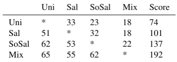
Uni Sal SoSal Mix Score
Uni * 33 23 18 74
Sal 51 * 32 18 101
SoSal 62 53 * 22 137
Mix 65 55 62 * 192
Table 6: Preference matrix for all the scenes combined.
5.2. Results
The results are shown in Table7. In all scenes where there was ambiguity in the grouping, more than one technique was grouped together. The Mix operator came top of every pref-erence table, had fewer discrepancies and was perceptually distinguishable statistically in two cases of testing whilst be-ing in the top group of the third case. It is also first in the overall and statistically significantly better than the other methods.
The coefficient of consistency in this experiment was
ζaverage≈0.75 and as such the participant’s consistency was deemed to be good and can all be included in the paired comparison study. The results provided anR+ (the smallest integer greater than R0) of 19. χ2d f=3,p<0.05 = 7.82,χ2d f=3,p<0.01=11.35,χ
2
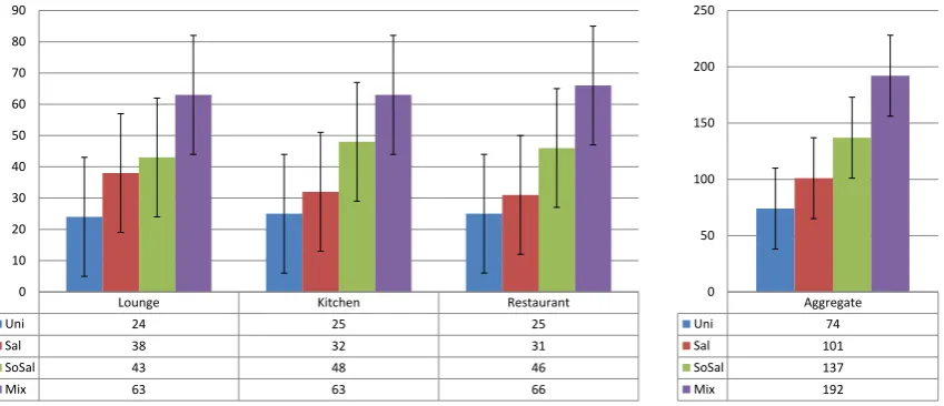
d f=3,p<0.001=16.27. This is shown against cumulative votes for each scene and aggre-gated in Figure 7. In addition the average coefficients of agreement and consistency are presented. As can be seen the results were perceptually distinguishable to a degree in all scenes. In all cases the null hypothesis is rejected and the multiple comparison range test can be used to find any pairwise difference scores equal to or greater thanR+to be significant.
Lounge Kitchen Restaurant
Uni 24 25 25
Sal 38 32 31
SoSal 43 48 46
Mix 63 63 66
0 10 20 30 40 50 60 70 80 90
Cu
m
u
lativ
e
Vo
te
s
Aggregate Uni 74 Sal 101 SoSal 137 Mix 192
0 50 100 150 200 250
Figure 7: Method Preference; Error bars indicate the rangeR+.
uaverage ζaverage χ2 P, df=3 Rank 1 Rank 2 Rank 3 Rank 4
Lounge 0.1658 0.7143 32.86 <0.05 Mix SoSal Sal Uni
Kitchen 0.1825 0.7571 35.57 <0.05 Mix SoSal Sal Uni
Restaurant 0.1975 0.7571 38.00 <0.05 Mix SoSal Sal Uni
All 0.1819 0.7428 35.47 <0.05 Mix SoSal Sal Uni
Table 7: Overall similarity study conclusion for the various scenes presented with spatialised acoustic stimuli and visual con-gruency’s.
significance level reported inP. As such, any declaration of grouping is stringently correct. In this case, whilst no clear cut group exists for every set, the fact that under the same render costs different sampling strategies report a perceptual difference is an important result. What is also interesting is that theauditory intensity mappresented in this paper also performs well, in the mid-range grouping with the Sal set. This is likely a result of the spatially encoded directional fea-tures of the audio. The answer may lie in temporal sensitivity of the HAS. However, this would require further investiga-tion.
6. Discussion
The performance expected from the auditory attention mod-els is limited by the features used in the modmod-els: intensity, frequency contrast, temporal contrast and cochlear response. Conventional auditory saliency models fail to perform tasks that require features which are not considered. For example, the model used in this paper uses monaural signals, and spa-tial cues are not considered. As a result, while the model is successful for tasks which are represented by at least one of the features of the model, it fails at the tasks which require
spatial cues, such as localisation and sound source separa-tion. This is accounted for by synergy between the presented auditory intensity map and auditory saliency feature vec-tors. The intensity map encodes features of saliency, locali-sation and separation in the visual domain that are not con-sidered by the auditory saliency model alone. A combination of the feature vectors, intensity map and visual saliency map formed the temporal hybrid auditory-visual domain model. As this model proposed in this paper is a bottom up model, assuming no task driven intervention, this means that the method should be effective regardless the sensory content, however further work would have to investigate the impact of tasks on this scenario.
7. Conclusions and Future Work
vi-sual saliency and auditory saliency in a selective rendering pipeline to temporally and dynamically load balance com-putation. The algorithm is psychophysically evaluated on a number of scenes, and across a number of render cost func-tions to evaluate its performance. It is shown to perform sig-nificantly better than simple image saliency or acoustic in-tensity maps when they are used as a rendering strategy and is generic in its formation and application. In visual-auditory VR environments the presented algorithm accounts for vi-sually important information when the auditory information presented is not deemed to be important and vice versa.
Future work will investigate the variability of the weight-ing function used across the different maps, especially in-vestigating the effect varying frequencies have upon sound and directional attentional capture. This type of map can-not, currently, be used for realtime processing in virtual en-vironments. The aim of the approach was to generate the auditory intensity map as a bi-product of the acoustic simu-lation step such that when hardware is more able to simulate closer to realtime the technique is more feasible. The type of simulation may be changed in the future to account for wave based effects of more recent sound simulation mod-els. Phonon tracing was deemed appropriate for the inherent practicality of the sound cache schema, but especially low frequency diffraction effects need to be better accounted for. The scene types could be more varied in order to draw more general conclusions, however in terms of the technique pre-sented, outdoor type scenes should be invariant to the results. It would be a logical progression to look into dynamic scenes with moving camera sequences and varying frequency light-ing. Sound could be tested presented spatially, decoding am-bisonics to 5.1 instead of binaural. Indeed even stereoscopic imagery could be an interesting tangent to the research. In evolutionary terms, certain sounds are more salient, and in fact, the pinna has the effect of amplifying these mid band frequencies down the auditory canal. In addition it is nec-essary to study the effect multiple sound sources have on visual attention. A first hypothesis would be the more salient source in the temporal domain would dominate spatially in the visual domain. A similar avenue of research is to study the intensity of the sound sources, specifically at which deci-bel level does the effect on visual attention come into play. Whilst the human ear can detect sound, the threshold of au-dibility remains true, but the effect to which salience takes precedence may not necessarily be linear in scale.
8. Acknowledgements
The authors would like to acknowledge EPSRC CASE stu-dentship award number 07001392 without which this work would not have been possible. Also, ARUP for keen indus-trial support and in particular Steve Walker. Finally, the au-thors would like to acknowledge Elmedin Selmanovic for his valuable input to this work.
References
[BDM∗05] BERTRAMM., DEINESE., MOHRINGJ., JEGOROVS
J., HAGENH.: Phonon tracing for auralization and visualization of sound.In Proceedings of IEEE Visualization(2005), 151–158. 2,3
[Bla97] BLAUERTJ.: Spatial Hearing : The Psychophysics of Human Sound Localization. M.I.T. Press, Cambridge, MA, 1997. 1
[BSVDD10] BONNEEL N., SUIED C., VIAUD-DELMON I.,
DRETTAKIS G.: Bimodal perception of audio-visual material
properties for virtual environments. ACM Trans. Appl. Percept. 7, 1 (2010), 1–16.1
[CCL02] CATERK., CHALMERSA., LEDDAP.: Selective qual-ity rendering by exploiting human inattentional blindness: look-ing but not seelook-ing. InVRST ’02(New York, NY, USA, 2002), ACM, pp. 17–24.1
[CDS∗09] COATH M., DENHAM S., SMITH L., HONING H., HAZANA., HOLONOWICZP., PURWINSH.: An auditory model for the detection of perceptual onsets and beat tracking in singing. Connection Science 21, 2 (2009), 193–205.6
[Coa05] COATHM.: A Computational Model of Auditory Fea-ture Extraction and Sound Classification. PhD thesis, Centre for Theoretical and Computational Neuroscience, University of Ply-mouth, 2005.6
[Dal] DALENBÄCKB.-I.: CATT-Acoustic, Gothenburg, Sweden. www.netg.se/catt.1
[Dal93] DALYS.: The visible differences predictor: an algorithm for the assessment of image fidelity. Digital images and human vision(1993), 179–206.6
[Dal98] DALYS.: Engineering observations from spatiovelocity and spatiotemporal visual models.Human Vision and Electronic Imaging III(1998), 180–191.2
[DM95] DURLACHN., MAVORA.:Virtual Reality Scientific and Technological Challenges. Tech. rep., National Research Council Report, National Academy Press, 1995.1
[DS98] DRIVERJ., SPENCEC.: Attention and the crossmodal construction of space. InTrends in Cognitive Sciences(1998), vol. 2, pp. 254–262.2
[FN05] FUJISAKIW., NISHIDAS.: Temporal frequency charac-teristics of synchrony-asynchrony discrimination of audio-visual signals.Exp Brain Res 166, 3-4 (October 2005), 455–464.4
[GBW∗09] GRELAUD D., BONNEEL N., WIMMER M., AS
-SELOTM., DRETTAKISG.: Efficient and practical audio-visual
rendering for games using crossmodal perception. InI3D ’09 (New York, NY, USA, 2009), ACM, pp. 177–182.1,3
[GLT05] GALLOE., LEMAITREG., TSINGOSN.: Prioritising signals for selective real-time audio processing. InProceedings of Intl. Conf. on Auditory Display (ICAD) 2005, Limerick, Ireland (July 2005).2
[HDAC10] HULUSIC V., DEBATTISTA K., AGGARWAL V.,
CHALMERSA.: Maintaining frame rate perception in interactive
environments by exploiting audio-visual cross-modal interaction. The Visual Computer(2010), 1–10.1,2
[HHT∗11] HULUSIC V., HARVEY C., TSINGOS N., DEBAT
-TISTAK., WALKERS., HOWARDD., CHALMERSA.: Acoustic
Rendering and Auditory-Visual Cross-Modal Perception and In-teraction. InEG 2011 - State of the Art Reports(2011), John N., Wyvill B., (Eds.), Eurographics Association, pp. 151–184.1
[HS36] HECHTS., SHLAERS.: Intermittent stimulation by light: The relation between intensity and critical frequency for different parts of the spectrum.Gen. Physiol. 19, 6 (jul 1936), 965–77.7 [HWBR∗10] HARVEY C., WALKER S., BASHFORD-ROGERS
T., DEBATTISTAK., CHALMERSA.: The Effect of Discretised and Fully Converged Spatialised Sound on Directional Attention and Distraction. InTPCG ’10(2010), Collomosse J., Grimstead I., (Eds.), Eurographics Association, pp. 191–198.2
[IKN98] ITTIL., KOCHC., NIEBURE.: A model of saliency-based visual attention for rapid scene analysis, 1998.2,6
[KBS40] KENDALLM., BABINGTON-SMITHB.: On the method of paired comparisons.Biometrika 31(1940), 324–345.9 [KDCM14] KOULIERISG. A., DRETTAKISG., CUNNINGHAM
D., MANIAK.: C-lod: Context-aware material level-of-detail applied to mobile graphics. Computer Graphics Forum 33, 4 (2014), 41–49.2
[KJM04] KAPRALOS B., JENKIN M., MILIOS E.: Acoustic modeling utilizing an acoustic version of phonon mapping. In Proc. of IEEE Workshop on HAVE(2004).3
[KPLL05] KAYSER C., PETKOV C. I., LIPPERT M., LOGO
-THETISN. K.: Mechanisms for allocating auditory attention:
An auditory saliency map. Current Biology 15, 21 (November 2005), 1943–1947.1,2,7
[LDC06] LONGHURSTP., DEBATTISTAK., CHALMERSA.: A gpu based saliency map for high-fidelity selective rendering. In ARFIGRPAH ’06(New York, NY, USA, 2006), ACM, pp. 21–29. 6
[MBT∗07] MOECKT., BONNEELN., TSINGOSN., DRETTAKIS
G., VIAUD-DELMONI., ALLOZAD.: Progressive perceptual audio rendering of complex scenes. InI3D ’07: Proceedings of the 2007 symposium on Interactive 3D graphics and games(New York, NY, USA, 2007), ACM, pp. 189–196.1,2
[MD02] MARMITTG., DUCHOWSKIA.: Modeling visual atten-tion in vr: Measuring the accuracy of predicted scanpaths. In Eurographics(2002), 217–226.1,2
[MDCT05a] MASTOROPOULOU G., DEBATTISTA K.,
CHALMERS A., TROSCIANKO T.: Auditory bias of visual
attention for perceptually-guided selective rendering of anima-tions. InGRAPHITE ’05(New York, NY, USA, 2005), ACM Press, pp. 363–369.1,2
[MDCT05b] MASTOROPOULOU G., DEBATTISTA K.,
CHALMERS A., TROSCIANKO T.: The influence of sound
effects on the perceived smoothness of rendered animations. In APGV ’05(New York, NY, USA, 2005), ACM Press, pp. 9–15. 1,2
[MMG11] MCNAMARAA., MANIAK., GUTIERREZD.: Per-ception in graphics, visualization, virtual environments and ani-mation. InSIGGRAPH Asia 2011 Courses(New York, NY, USA, 2011), SA ’11, ACM, pp. 17:1–17:137.2
[Moo97] MOOREB. C.: An introduction to the psychology of hearing. Academic Press, 4th edition, 1997.2
[Nay93] NAYLORJ.: ODEON - another Hybrid Room Acoustical Model.Applied Acoustics 38, 1 (1993), 131–143.1
[Pet99] PETTERSSONR.: Attention an information design per-spective! International Institute for Information Design (IIID), Vienna, Austria, 1999.1
[PS00] PAINTERE. M., SPANIASA. S.: Perceptual coding of digital audio.Proceedings of the IEEE 88, 4 (april 2000).2 [RBF08] RAMANARAYANANG., BALAK., FERWERDAJ. A.:
Perception of complex aggregates. InSIGGRAPH ’08: ACM SIGGRAPH 2008 papers(New York, NY, USA, 2008), ACM, pp. 1–10.1
[RFWB07] RAMANARAYANANG., FERWERDAJ., WALTERB., BALAK.: Visual equivalence: towards a new standard for image fidelity.ACM Trans. Graph. 26, 3 (2007), 76.1
[RLC∗07] RAGHUVANSHIN., LAUTERBACHC., CHANDAKA.,
MANOCHAD., LINM. C.: Real-time sound synthesis and
prop-agation for games.Commun. ACM 50, 7 (2007), 66–73.1 [SLKS07] SILTANENS., LOKKIT., KIMINKIS., SAVIOJAL.:
The room acoustic rendering equation. J. Acoust. Soc. Am. 122, 3 (Sep 2007), 1624–1632.3
[Sur12] SURFACES A.: Sound absorbtion coefficients. World Wide Web electronic publication, 2012.6
[TGD04] TSINGOSN., GALLOE., DRETTAKISG.: Perceptual audio rendering of complex virtual environments. ACM Trans. Graph. 23, 3 (2004), 249–258.1
[Tsi05] TSINGOSN.: Scalable perceptual mixing and filtering of audio signals using an augmented spectral representation. Proc. of 8th Intl. Conf. on Digital Audio Effects (DAFX’05), Madrid, Spain(Sept. 2005).2
[WW80] WELCH R., WARREND.: Immediate perceptual re-sponse to intersensory discrepancy. InPsychological Bulletin (nov 1980), vol. 88(3), pp. 638–667.2
[Yee00] YEEY. L. H.: Spatiotemporal sensitivity and visual at-tention for efficient rendering of dynamic enivroments. PhD the-sis, Cornell University, Aug 2000.2