Article
Advancing the AirMOSS P-Band Radar Root Zone
Soil Moisture Retrieval Algorithm via Incorporation
of Richards’ Equation
Morteza Sadeghi 1,*, Alireza Tabatabaeenejad 2, Markus Tuller 3, Mahta Moghaddam 2 and Scott B. Jones 1
1 Department of Plants, Soils and Climate, Utah State University, Logan, UT 84322, USA; scott.jones@usu.edu
2 Ming Hsieh Department of Electrical Engineering, University of Southern California, Los Angeles, CA 90089, USA; alirezat@usc.edu (A. T.), mahta@usc.edu (M. M.)
3 Department of Soil, Water and Environmental Science, The University of Arizona, Tucson, AZ 85721, USA; mtuller@cals.arizona.edu
* Correspondence: morteza.sadeghi@usu.edu; Tel.: +1-435-554-5369
Abstract: P-band radar remote sensing applied during the Airborne Microwave Observatory of Subcanopy and Subsurface (AirMOSS) mission has shown great potential for estimation of root zone soil moisture. When retrieving the soil moisture profile (SMP) from P-band radar, a mathematical function describing the vertical moisture distribution is required. Because only a limited number of observations are available, the number of free parameters of the mathematical model must not exceed the number of observed data. For example, a second order polynomial that contains 3 free parameters was presumed based on in-situ SMP data. The polynomial is currently parameterized based on 3 backscatter observations provided by AirMOSS (i.e. one frequency at three polarizations of HH, VV and HV). In this paper, a more realistic, physically-based SMP model containing 3 free parameters is derived based on a solution to Richards’ equation for unsaturated flow in soils. Evaluation of the new SMP model based on both numerical simulations and measured data revealed that it exhibits greater flexibility for fitting measured and simulated SMPs than the currently applied polynomial. It is also demonstrated that the new SMP model can be reduced to a second order polynomial at the expense of fitting accuracy.
Keywords: AirMOSS; radar backscatter; P-band remote sensing; root zone; soil moisture profile; Richards’ equation
1. Introduction
Soil moisture is a key state variable controlling all major processes and feedback loops within the climate system. Soil moisture impacts the water and energy cycles and the exchange of trace gases, including carbon dioxide, between land and atmosphere [1]. A number of high-profile review articles published in recent years [1–5] highlight the crucial importance of spatial and temporal soil moisture information at various scales for virtually all hydrologic, atmospheric, and ecological processes.
Remote sensing (RS) has demonstrated great potential for large-scale monitoring of soil moisture utilizing various frequency bands of the electromagnetic spectrum such as shortwave infrared [6,7], thermal infrared [8–10], or microwave radiation [11,12]. Microwave RS techniques have shown greater promise for global monitoring of soil moisture variations [13], because in contrast to thermal and optical RS, they are not impacted by clouds and solar radiation and there is significant penetration into the soil and overlying vegetation at lower microwave frequencies [11].
Subsurface” (AirMOSS) mission provides an unprecedented sensing depth of about 50 cm to directly retrieve root zone soil moisture under vegetation canopies [14].
When retrieving the soil moisture profile (SMP) from P-band radar, a mathematical function describing the continuous SMP is required. Because inevitably only a limited number of observations are available, the number of free parameters of the mathematical model must not exceed the number of observed data to ensure unambiguous retrievals. For example, in the current AirMOSS P-band radar root zone soil moisture retrieval algorithm a second order polynomial (hereinafter referred to as polynomial) with 3 free parameters is presumed and parameterized based on 3 backscatter observations provided by AirMOSS (i.e. one frequency at three polarizations of HH, VV and HV) [14]. To improve AirMOSS SMP retrieval, the objective of this study was to derive a more realistic and physically-based SMP model via solving Richards’ equation (RE) for unsaturated flow in soils [15].
Due to the highly nonlinear nature of flow processes in unsaturated soils, analytical solutions to RE are commonly restricted to simple cases such as a linearized form of RE [16–18] or steady-state Darcy flow [19–22]. However, these simplified cases rarely meet realistic soil and environmental conditions, where after wetting events (i.e., precipitation or irrigation) the most common flow scenario encompasses concurrent drying due to evaporation of water from the soil surface and gravity-driven movement of water to greater depths within the soil profile.
Existing analytical solutions to RE for the abovementioned process are restricted to simplified cases. For example, solutions introduced by Gardner [23], Novak [24], and Suleiman and Ritchie [25] were obtained by reducing the RE to a diffusion-type partial differential equation neglecting gravity-driven flow. Analytical solutions of Warrick [16] and Teng et al. [26] were obtained by linearization of the RE based on assuming an exponential saturation-pressure head and linear saturation-hydraulic conductivity relationships, which is rarely met under natural conditions.
Warrick et al. [27] based on the analysis of Broadbridge and White [28] introduced to our best knowledge the only analytical solution to the nonlinear RE for the case of evaporation and concurrent drainage. However, this solution (Eq. 26 in [27]) is not applicable for AirMOSS SMP retrieval because it consists of more than 3 free parameters (considering time as a constant in the solution to fit snapshot observations at any given time).
In the following, a simple closed-form analytical solution to the nonlinear RE containing 3 free parameters is introduced. The solution is presented in a general form, not limited to specified initial and boundary conditions. The free model parameters are obtained via nonlinear regression analysis of measured data. As a result, the solution can be fitted to SMP data observed for either evaporation/drainage or infiltration. Theoretical aspects for derivation of the new solution and its validation based on measured and numerically simulated data are presented.
2. Mathematical Derivations
2.1. Richards’ Equation
Richards’ equation (RE) [15] combines the Buckingham-Darcy law [29], q = –K(∂h/∂z – 1), and the continuity principle, ∂θ/∂t = –∂q/∂z (conservation of mass):
h
K
K
t
z
z
θ
∂
∂
∂
=
−
∂
∂
∂
(1)where q is the water flux density, θ is the soil water content, h is the pressure head, K is the unsaturated hydraulic conductivity, t is time, and z is soil depth assumed positive downward from the soil surface.
In an unsaturated soil, h and K are functions of θ which are assumed to be invariant for a given soil, but may distinctly deviate for different soils. Various mathematical relationships exist for the soil hydraulic h(θ) and K(θ) functions [e.g. 30–32] that are commonly parameterized via nonlinear regression analysis of measured h-θ and K-θ data for a soil of interest.
To obtain an analytical solution for Eq. (1), the following soil hydraulic functions are assumed [33,34]:
(
)
exp
/
(
)
r s r
h Ph
cMθ θ
= +
θ θ
−
−
(2) P r s s rK K
θ θ
θ θ
−
=
−
(3)where θs and θr are the saturated and residual volumetric water contents, respectively, Ks is the
saturated hydraulic conductivity, P is an empirical parameter related to soil pore size distribution, and hcM is the effective capillary drive introduced by Morel-Seytoux and Khanji [35]. Assuming P = 1,
the RE is reduced to a linearized form for which analytical solutions to various flow processes exist [16-18]. However, the assumption P = 1 is rarely met in reality; most soils exhibit a P significantly larger than 1 [33]. Thus, P is treated as a soil parameter in the following derivations, where the resulting nonlinear RE is solved analytically. Note that the soil hydraulic parameters θs, θr, P, Ks, and
hcM are constant for a given soil and do not change with time. Therefore, they should be discerned
from the so-called “free parameters”, which vary temporally to fit the SMP at any given time. For convenience, variables are reduced to the following dimensionless forms:
*
/
cM
h
=
h h
(4)(
) (
)
*
/
r s r
θ
= −
θ θ
θ θ
−
(5)*
/
s
K
=
K K
(6)*
/
cM
z
=
z h
(7)(
)
*
/
s cM s r
t
=
K t
h
θ θ
−
(8)Substituting Eqs. (4) to (8) into Eq. (1) yields a scaled form of the RE:
* *
* *
* * *
h
K
K
t
z
z
θ
∂
=
∂
∂
−
∂
∂
∂
(9)with the following scaled soil hydraulic functions:
(
)
*
exp
h P
*/
θ
=
(10)* *P
K
=
θ
(11)Combining Eqs. (9), (10), and (11) yields the scaled RE rearranged based on K*:
(1 1/ )
2
* 2 * *
*
* * *
P
K
K
K
PK
t
z
z
−
∂
=
∂
−
∂
∂
∂
∂
(12)Assuming P >> 1 (i.e. 1 – 1/P ≈ 1) as is the case in many natural soils (see Table 1 in [33] as well as Table 1 in this paper), Eq. (12) can be approximated as:
2
* 2 * *
*
* * *
K
K
K
PK
t
z
z
∂
=
∂
−
∂
∂
∂
∂
(13)To solve Eq. (13), separation of variables is applied:
( ) ( ) ( )
* *
,
* * *K z t
=
F z G t
(14)Combining Eqs. (13) and (14) yields:
2
2
2 * * *
1
constant
dG
d F
dF
PG dt
=
dz
−
dz
= =
μ
(15)2
2
*
*
0
d F
dF
dz
dz
−
− =
μ
(16)2
*
0
dG
PG
dt
−
μ
=
(17)Solutions to Eqs. (16) and (17) are:
* *
1
exp( )
2F
= −
μ
z
+
a
z
+
a
(18)* 3
1
G
Pt
a
μ
=
−
+
(19)where a1, a2, and a3 are the integral constants. Combining Eqs. (14), (18) and (19), and denoting the constants b1, b2, and b3, a simple closed-form solution is obtained:
* *
* * * 1 2
* 3
exp( )
exp
P
z
b
z
b
K
h
Pt
b
θ
+
+
=
=
=
+
(20)Because AirMOSS observations are temporally not continuous but rather provide snapshots at specific times, time needs to be considered as a constant. This consideration together with the assumption that θr is negligibly small allows transformation of Eq. (20) to the final SMP solution:
(
)
1/1 2
exp
/
3P cM
c z c
z h
c
θ
=
+
+
(21) where c1, c2, and c3 are the combined constants or the final free parameters of the RE-based SMP model.
It should be noted that because of the exponential/power nature of Eq. (21), the derived SMP model is highly sensitive to variations of free model parameters (i.e., small changes in c1, c2, and c3 lead to a significant change of the SMP shape). This means that direct derivation of c1, c2, and c3 through inversion is not as straightforward as proposed in [14], for example, to find the optimum polynomial parameters. However, this problem can be resolved in the inversion algorithm by finding the optimum values of soil moisture at three arbitrary depths, θ1(z1), θ2(z2), and θ3(z3), instead of optimizing c1, c2, and c3. Then the model parameters can be calculated directly as:
(
)
(
)
3 1 2 1
1
3 1 2 1
P P
A
P Pc
z
z
A z
z
θ
−
θ
−
θ
−
θ
=
− −
−
(22)
(
)
(
2 1)
1 2(
1)
2
2 1
exp
/
exp
/
P P
cM cM
c z
z
c
z h
z h
θ
−
θ
−
−
=
−
(23)(
)
3 1 1 1 2
exp
1/
P
cM
c
=
θ
−
c z c
−
z h
(24)where:
(
)
(
)
(
)
(
)
3 1
2 1
exp
/
exp
/
exp
/
exp
/
cM cM
cM cM
z h
z h
A
z h
z h
−
=
−
(25)2.3. Second Order Polynomial Approximation
At the expense of fitting flexibility, Eq. (21) can be simplified with the assumption that P = 1:
(
)
1 2
exp /
cM 3c z c
z h
c
θ
=
+
+
(26)A Taylor series expansion yields:
2 3
1
1
exp
1
...
2!
3!
cM cM cM cM
z
z
z
z
h
h
h
h
= +
+
+
+
For hcM larger than the maximum depth of interest (i.e. z/hcM < 1), all the terms with orders higher than
2 can be neglected. Hence Eq. (26) can be reduced to the polynomial presumed in [14]:
2
2
1 2 3
1
1
2
cM cM
z
z
c z c
c
az
bz c
h
h
θ
=
+
+
+
+ =
+ +
(28)
Equation (28) implicates that the second order polynomial introduced in [14] based on empirical findings can be approximated based on the physics of unsaturated flow in soils. The accuracy of this approximation is dependent on the SMP shape, which is discussed in the following section.
3. Validation of the proposed SMP model 3.1. Numerical Data
To explore the flexibility of Eq. (21) to match realistic SMPs, the original RE was solved numerically with the HYDRUS-1D simulation model [36]. To account for the soil moisture vaporization plane recession during the second stage of the drying process [37], vapor flow coupled with the RE was also considered in the numerical simulations.
The most common unsaturated flow scenario in nature, evaporation of water from the soil surface, was simulated concurrently with downward water redistribution along the soil profile after a wetting event (rainfall/irrigation). Therefore, free drainage at the bottom boundary (z = 50 cm in the presented simulations) and atmospheric conditions at the top boundary with a potential evaporation rate of 0.5 cm day-1 and atmospheric pressure head of −100 m were assumed. To simulate the drying process after a wetting event, the initial soil profile was assumed to be saturated from z = 0 to 30 cm and air-dry from z = 30 to 50 cm. Hydraulic properties of three vastly different soil textures including sand, loam and clay were used to parameterize the HYDRUS simulations. The van Genuchten (VG) [30] soil hydraulic functions were applied with HYDRUS default soil hydraulic parameters listed in Table 1:
[1 (
) ]
n m eS
= +
α
h
− (29)(
)
20.5
1 1
1/m ms e e
K
=
K S
− −
S
(30)where α, n, and m are VG model parameters assuming m = 1 − 1/n.
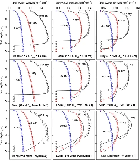
Figure 1 (top row) depicts the HYDRUS simulation results for each of the three textures at three different drying times as well as the best fits of Eq. (21). To find the optimum values of P and hcM for
each soil (presented in each plot), first an initial guess was made. Then three arbitrary data points,
θ1(z1), θ2(z2), and θ3(z3), from the Hydrus simulations were used to calculate c1, c2, and c3 with Eqs. (22) to (25). Finally, P and hcM were optimized to best fit the simulation results.
Figure 1 (top row) illustrates how well the new SMP solution, Eq. (21), fits numerical data. It is apparent that all assumptions that were required to derive the analytical SMP solution (e.g. soil hydraulic functions of Eq. (2) and (3)) are highly suitable when Eq. (21) is employed as a fitting curve rather than a predictive tool (e.g., common RE solutions to simulate SMP at different times along a specific initial/boundary value problem).
Soil water content (cm3 cm-3)
0.0 0.1 0.2 0.3
Soi
l de
pth (cm)
0
10
20
30
40
50
Sand (P = 4.5, hcM = 4.2 cm) 0.01 day
0.1 day 1 day
So
il depth (
cm)
0
10
20
30
40
50
0.01 day
0.1 day
1 day
Soi
l d
epth
(c
m)
0
10
20
30
40
50
0.01 day
0.1 day 1 day
Soil water content (cm3 cm-3)
0.1 0.2 0.3 0.4 0.1 day
1 day
30 day
Soil water content (cm3 cm-3)
0.25 0.30 0.35 0.40
1 day
30 day
365 day
0.1 day
1 day 30 day
1 day
30 day
365 day
Loam (P = 6.6, hcM = 87.0 cm) Clay (P = 15.9, hcM = 350.0 cm)
Sand (P and hcM from Table 1)
Sand (2nd order Polynomial)
Loam (P and hcM from Table 1) Clay (P and hcM from Table 1)
1 day 30 day
365 day
Clay (2nd order Polynomial) 0.1 day
1 day
30 day
Loam (2nd order Polynomial)
Figure 1. The best fit of Eq. (21) (solid lines) to HYDRUS-1D simulation results (circles) for simultaneous evaporation and drainage in three different soils. The soil parameters, P and hcM, were treated as fitting parameters (top row), taken from Table 1 (middle row), or were considered as P = 1 and hcM >> 50 cm leading to the second order polynomial (bottom row). Data below the wetting front were not considered for nonlinear regression analysis.
The SMP model, Eq. (21), includes 2 soil parameters and 3 free parameters. Therefore, for application in the AirMOSS algorithm that only allows 3 free parameters, the soil parameters should be known. Determination of the soil hydraulic parameters (P and hcM) requires measurement of the
(
)
1(
1/)
0.5 2 ln 0.5
ln 1
1 0.5
m mP
=
+
−
− −
(31)( )
1(
)
1/exp 1/
1
ncM
h
=
α
P
−
m
−
(32) Equations (31) and (32) were derived from equivalence of Eq. (2) and (3) with Eqs. (29) and (30) such that they yield the same θ* at h = P × hcM and the same K at θ* = 0.5. These equations are introduced
here because average VG parameters for various textures are well documented in the literature [40] (Table 1) and they can be approximated with pedotransfer functions from easy-to-measure textural properties (sand, silt and clay percentages) [41]. The calculated parameters P and hcM based on Eqs.
(31) and (32) with VG parameters provided in [40] for the 12 USDA soil textural classes are listed in Table 1.
Fitting of Eq. (21) with values from Table 1 is also depicted in Fig. 1 (middle row). It is evident that these values generally lead to a reasonable fit of Eq. (21) to numerical data. Nonetheless, the parameters for the clay soil seem to be much higher than the best fitting parameters presented earlier. This is due to the fact that Eqs. (2) and (3) substantially deviate from the VG functions for clayey soils. Hence, for the two last soils of Table 1 (silty clay and clay) we recommend P = 15.9 and hcM = 350 cm
rather than values listed in Table 1.
Table 1. Average van Genuchten model parameters for the 12 USDA soil textural classes [40] as well as parameters for Eqs. (2) and (3) calculated with Eqs. (31) and (32).
Soil texture θr θs α
(cm–1) n
Ks
(cm/day) P
hcM
(cm)
Sand 0.045 0.43 0.145 2.68 712.80 4.83 2.38
Loamy sand 0.057 0.41 0.124 2.28 350.20 5.52 2.94 Sandy loam 0.065 0.41 0.075 1.89 106.10 6.73 5.70
Loam 0.078 0.43 0.036 1.56 24.96 8.89 17.90
Silt 0.034 0.46 0.016 1.37 6.00 11.60 78.94
Silt loam 0.067 0.45 0.020 1.41 10.80 10.84 51.64 Sandy clay loam 0.100 0.39 0.059 1.48 31.44 9.79 13.46 Clay loam 0.095 0.41 0.019 1.31 6.24 13.05 100.39 Silty clay loam 0.089 0.43 0.010 1.23 1.68 16.00 481.18 Sandy clay 0.100 0.38 0.027 1.23 2.88 16.00 178.22 Silty clay 0.070 0.36 0.005 1.09 0.48 31.92 4.19E5
Clay 0.068 0.38 0.008 1.09 4.80 31.92 2.62E5
Figure 1 (bottom row) also depicts the fitted polynomial, Eq. (28), to the numerical data. It is apparent that the polynomial does not capture numerical data at earlier stages of evaporation well, but performs reasonably well at later times when the SMP becomes drier. A main reason for losing accuracy of Eq. (21) when reduced to the polynomial is that parameters of P = 1 and hcM > 50 cm are
assumed in this case. Based on values shown in Table 1, it is unlikely to find a natural soil which meets this condition, since P = 1 corresponds to an extremely coarse-textured soil and large hcM
corresponds to a fine-textured soil. This mismatch highlights the advantage of using the general model, Eq. (21), rather than its reduced form, Eq. (28), in the AirMOSS algorithm.
shown in Fig. 1 (top row). Equation (21) would certainly better match numerical data if P and hcM
were adjusted. However, P and hcM were assumed constant as they should be for any given soil,
regardless of the flow process. The discrepancies are due to the simplifying assumptions for derivation of Eq. (21).
Soil water content (cm3 cm-3)
0.1 0.2 0.3 0.4
S
o
il de
p
th (cm
)
0
5
10
15
20
25
1 hour 2 hour
5 hour
Loam (P = 6.6, hcM = 87.0 cm)
Figure 2. The best fit of Eq. (21) (lines) to HYDRUS-1D simulation results (circles) for a constant-flux (= 1 cm h-1) infiltration process into a loam soil with parameters given in Table 1.
3.2. Measured Data
We also tested the fitting accuracy of the proposed SMP model to real measurements from the Soil Climate Analysis Network (SCAN) [42]. As a first test case, SCAN site number 2078 in Madison, Alabama, which was also used in Mishra et al. [43] was considered. Mishra et al. [43] found the SCAN data to provide ideal test cases for evaluating fitting capabilities of their proposed SMP model. They indicated that two general shapes of soil moisture profiles are commonly observed in course of the drying process: (i) the “dynamic case”, which is analogues to earlier times of drying shown in Fig. 1; and (ii) the “dry case”, which is similar to the late drying times in Fig. 1.
Figure 3 compares the fitting capabilities of Eq. (21) (new solution) and Eq. (28) (polynomial) to measured soil moisture data exhibiting the dynamic case. Since the soil texture of the SCAN site is predominantly clay, P = 15.9 and hcM = 350 cm were used for Eq. (21). For both Eqs. (21) and (28) it
was assumed that below the dynamic zone the water content is uniform and equal to that of the wetting front. It is well documented that at later evaporation stages, a dry zone develops close to the soil surface and the so-called drying front (or vaporization plane) recedes below the surface. In this case, the Buckingham-Darcy law is not applicable for modeling soil water content above the drying front without accounting for the vapor flow contribution, because the pressure head gradient approaches infinity at the drying front [44]. Therefore, it was assumed for Eq. (21) that soil water content above the drying front (i.e. where Eq. (21) intersects θ = 0) is zero.
Soil water content (cm3 cm-3)
0.1 0.2 0.3 0.4
Soil d
epth
(c
m
)
0
20
40
60
80
100
Soil water content (cm3 cm-3)
0.1 0.2 0.3 0.4 0
20
40
60
80
100
Eq. (21), P = 15.9 Eq. (21), P = 11 Polynomial Measured
JD = 31 JD = 40
FC
PW
P FC
PW
P
Figure 3. The best fit of Eqs. (21) (new solution) and Eq. (28) (second order polynomial) to measured soil moisture data from SCAN site number 2078 (Madison, Alabama) at Julian days (JD) 31 and 40, 2013. The clay soil parameters, P = 15.9 (or 11 for a comparison) and hcM = 350 cm, were used for fitting Eq. (21).
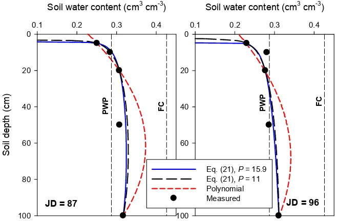
The comparisons for the dry case are shown in Fig. 4. It is evident that the polynomial when compared with the RE solution overpredicts water content at most depths, especially within the dry zone near the soil surface. Equation (21) predicts formation of a dry layer down to about 3-4 cm. This prediction is plausible, because the water content of the entire profile is close to the permanent wilting point (PWP) (i.e., water content at h = −15 m).
Soil water content (cm3 cm-3)
0.1 0.2 0.3 0.4
Soil d
epth
(c
m
)
0
20
40
60
80
100
Soil water content (cm3 cm-3)
0.1 0.2 0.3 0.4 0
20
40
60
80
100
Eq. (21), P = 15.9 Eq. (21), P = 11 Polynomial Measured
JD = 87 JD = 96
FC
PW
P FC
PW
P
Figure 4. The best fit of Eqs. (21) (new solution) and Eq. (28) (second order polynomial) to measured soil moisture data from SCAN site number 2078 (Madison, Alabama) at Julian days (JD) 87 and 96, 2012. The clay soil parameters, P = 15.9 and P = 11 (for comparison) and hcM = 350 cm, were used for fitting Eq. (21).
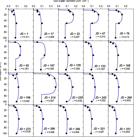
the sites studied for AirMOSS evaluation in Tabatabaeenejad et al. [14]. To evaluate to what extent Eq. (21) can capture SMP seasonal dynamics, biweekly data over one year were used for this analysis. The soil profile at this site is not uniform, consisting of various textures (loam, loamy sand, sandy loam) down to a depth of 1 m. Nonetheless, we evaluated Eq. (21) assuming a uniform profile by applying the loam soil parameters, P = 6.6 and hcM = 87 cm.
Results of this test are presented in Fig. 6, verifying that Eq. (21) is able to adequately capture seasonal SMP dynamics, even with roughly approximated soil parameters for the heterogeneous soil profile. The estimated profiles could certainly be different from reality due to the lack of observations at the surface (z = 0) or missing information about the exact location of the wetting front. Nonetheless, the estimated dynamics are consistent with common observations (e.g. Fig. 1) showing a similar pattern for damping the wetted zone formed after a wetting event (e.g. at JD of 32 and 214) over time.
0.0 0.1 0.2
Soi
l d
epth (
cm)
0
20
40
60
80
100
0.0 0.1 0.2
Soil water content (cm3 cm-3)
0.0 0.1 0.2 0.0 0.1 0.2 0.0 0.1 0.2
0
20
40
60
80
100 0
20
40
60
80
100 0
20
40
60
80
100
JD = 1 JD = 17 JD = 32 JD = 47 JD = 76
JD = 92 JD = 107 JD = 129 JD = 153 JD = 168
JD = 198 JD = 214 JD = 229 JD = 245 JD = 260
JD = 275 JD = 290 JD = 306 JD = 321 JD = 351
ε = 0.011 ε = 0.008 ε = 0.007 ε = 0.010 ε = 0.012
ε = 0.001 ε = 0.000 ε = 0.005 ε = 0.007 ε = 0.008
ε = 0.020 ε = 0.007 ε = 0.009 ε = 0.002 ε = 0.006
ε = 0.005 ε = 0.006 ε = 0.006 ε = 0.007 ε = 0.008
4. Inversion Considerations
In the current AirMOSS retrieval algorithm, the SMP is retrieved from estimation of the free parameters a, b and c in Eq. (28). A “simulated annealing” algorithm based on the work of Corana et al. [45] is used to minimize a cost function that is based on the difference between measured and calculated backscattering coefficients. At each iteration of a, b, and c in the inversion algorithm, soil moisture is calculated at all depths with Eq. (28). Then the dielectric constant at each soil depth is calculated as a function of its moisture content, and finally the backscattering coefficient is calculated for each set of a, b and c coefficients. The optimum parameter set that minimizes the difference between measured and calculated backscattering coefficients is selected to yield the retrieved SMP from Eq. (28). The choice of initial guesses is not of concern as global optimization techniques, such as the simulated annealing algorithm used for AirMOSS retrievals, are insensitive to initial guesses of free model parameters [14].
The P-band retrieval algorithm of AirMOSS currently uses only the HH and VV channels due to calibration inaccuracy of the HV channel. Therefore, the corresponding inverse problem is ill-posed as 3 free parameters are retrieved with only 2 data points. Some regularization is thus necessary to overcome the effect of the ill-posedness. The method applied by Tabatabaeenejad et al. [14] is based on defining upper and lower bounds for each free parameter according to available in-situ soil moisture data at each AirMOSS site. Considering the polynomial assumption, in-situ measured soil moisture profiles at each site are fitted with a quadratic function and the free parameters are observed throughout the year. An upper and lower bound is empirically selected for each flight date based on the behavior of the free parameters within the time period encompassing the flight date. In addition to mathematical inaccuracies in the forward and inverse models, the physics of the problem (i.e., penetration depth of the electromagnetic waves) also imposes a limitation on retrieval accuracy. AirMOSS has assumed a validation depth of up to 50 cm in its retrieval algorithm. This depth makes the soil homogeneity assumption (underlying the new solution) valid should the presented new RE solution be used for similar future retrievals [14].
When employing the new solution, Eq. (21), in the AirMOSS algorithm, θ1, θ2 and θ3 at three fixed depths (z1, z2 and z3)are optimized instead of a, b and c. Therefore, the problem of finding the upper and lower bounds is more straightforward because of the physical meaning of θ1, θ2 and θ3 from which free parameters of Eq. (21) can be directly calculated with Eqs. (22), (23) and (24).
Although initial and boundary conditions were not specified for derivation of the new solution to the RE, it should be noted that Eq. (21) only holds for simple cases such as uniform initial conditions or time-invariant boundary conditions. Any solution for non-uniform initial conditions or transient boundary conditions would include additional free parameters dealing with the mathematical description of the space- or time-varying conditions. To better understand this point, three possible arrangements of θ1, θ2 and θ3 shown in Fig. 6 are discussed below.
Case A is similar to early drying times for which θ2 > θ1 and θ3. Equation (21) is always valid for this case. Case B is similar to later drying times for which θ3 > θ2 > θ1. Equation (21) is valid for this case, unless θ3 is larger than a critical value θc. The critical value can be approximated with Eq. (33)
that ensures validity of Eq. (21) in most cases:
(
)
1/1 2 1
P
P P P
c
A
θ
≈
θ
−
θ θ
−
(33)The constraint of θ3 < θc is necessary for inversion from a mathematical point of view, although the
condition θ3 > θc is rarely observed in natural settings. Therefore, the new solution can be easily
applied to the profiles of cases A and B. These two cases can be merged into a single case when the two constraints of θ1 < θ2 and θ3 < θc are satisfied.
Case C for which θ2 < θ1 and θ3, however, cannot be predicted with Eq. (21), as θ is undefined within part of the profile where c1 z + c2 exp (z/hcM) + c3 is negative. For such case, it is suggested to
release the two constraints for cases A and B and rather assume P = 1 in order to replace Eq. (21) with Eq. (26), which is approximately the same as the polynomial, Eq. (28), as indicated in Fig. 6.
Soil water content (cm3 cm-3)
0.00 0.02 0.04 0.06 0.08
S
oil d
ept
h (cm)
0
10
20
30
40
50
Soil water content (cm3 cm-3)
0.00 0.04 0.08 0.12
Eq. (21) Eq. (26) Eq. (28) Measured
Soil water content (cm3 cm-3)
0.00 0.05 0.10 0.15 0.20 0.25
Undefined
θ1
θ2
θ3
θ1
θ2
θ3
θ1
θ2
θ3
Case A Case B Case C
Fig. 6. Three possible arrangements of θ1, θ2 and θ3 throughout the drying process. Data were extracted from Fig. 13a in Tabatabaeenejad et al. [14]; profile 2 (case A), profile 6 (case B) and profile 4 (case C). Values of P = 6.6 and hcM = 87 cm were assumed.
5. Preliminary Inversion Results
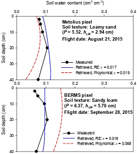
As a preliminary test of the new solution, we present sample inversion results from two AirMOSS flights; one flight over Metolius on August 21, 2015 and a second over BERMS on September 28, 2015. We observed that the behavior of one of the installed probes at each site can be categorized as case A or B for at least a 50-day period encompassing the flight dates. We applied the inverse algorithm for the radar data for these two flights and compared the retrieval errors with those obtained from the current AirMOSS algorithm that is based on the polynomial function assumption (Fig. 7). The Metolius pixel has a loamy sand soil with P = 5.52 and hcM = 2.94 cm, and the BERMS
Soil water content (cm3 cm-3)
0.0 0.1 0.2 0.3 0.4
Soil de
pth (c
m)
0
10
20
30
40
Measured
Retrieved, RE: ε = 0.017 Retrieved, Ploynomial: ε = 0.019
Metolius pixel
Soil texture: Loamy sand (P = 5.52, hcM = 2.94 cm) Flight date: August 21, 2015
0.0 0.1 0.2 0.3 0.4
Soil de
pth (c
m)
0
10
20
30
40
Measured
Retrieved, RE: ε = 0.018 Retrieved, Ploynomial: ε = 0.068
BERMS pixel
Soil texture: Sandy loam (P = 6.37, hcM = 5.70 cm) Flight date: September 28, 2015
Fig. 7. AirMOSS retrieved soil moisture profiles using the new solution (RE) and second order polynomial for two flights over Metolius on August 21, 2015 and over BERMS on September 28, 2015. Inversion accuracy is quantified by the mean absolute error, ε (cm3 cm−3).
It is evident that the retrieval errors have decreased when representing the soil moisture profile with the new RE solution. The computational inversion time also decreased by about 20% for both cases. Unless an extensive error comparison for several AirMOSS sites and several dates is performed, it is not possible to firmly claim that the error reduction (Fig. 7) and computational time savings hold for all cases. However, for these two specific cases, we believe the error reduction can be attributed to two factors. First, the unknowns of the new solution are physical parameters. Therefore, the corresponding lower and upper bounds can be deduced with more confidence from in-situ data when compared to the second order polynomial. Second, as discussed earlier, the SMP function is less sensitive to changes, hence uncertainty, in θ1, θ2 and θ3 than the polynomial is to changes in the coefficients a, b and c, which are in fact a special case of c1, c2 and c3.
We acknowledge that this method has its own limitation when compared to the current AirMOSS method. One limitation is the requirement of a priori information about the SMP shape (i.e., whether it is case C or not). When there is no a priori information about the SMP shape (e.g., in-situ observations), a possible solution to this limitation would be first assuming that the profile shape satisfies cases A or B, thus holding the required constraints (i.e., θ1 < θ2 and θ3 < θc). For the case that
the error between measured and calculated backscattering coefficients cannot be satisfactorily minimized with these constrains, case C can then be assumed (i.e., P = 1).
6. Conclusions
Equation (21), a closed-form analytical solution to Richards’ equation, is proposed as an alternative to the second order polynomial that is currently employed in the Airborne Microwave Observatory of Subcanopy and Subsurface (AirMOSS) root zone soil moisture retrieval algorithm. It has been demonstrated that the second order polynomial is a special case of Eq. (21) limited to P = 1. Evaluation of Eq. (21) based on both numerical simulations and measured data revealed that it exhibits greater flexibility than the currently applied second order polynomial. Therefore, application of Eq. (21) is recommended for more accurate retrieval of root zone moisture profiles from P-band radar remote sensing data. The results presented for two AirMOSS flights in 2015 demonstrate a reduction of the retrieval error with the new method. In conclusion it should be noted that while the retrieval error and computational inversion time have improved for the two presented cases, a more extensive study is required to investigate the applicability, performance, and advantage of this method for AirMOSS root-zone soil moisture retrievals.
Acknowledgments: We acknowledge funding from the National Science Foundation (NSF) grant no. 1521469 awarded to Utah State University and to the University of Arizona. Support of the National Aeronautics and Space Administration (NASA) AirMOSS EVS-1 mission under a contract to the University of Southern California is also gratefully acknowledged. Additional support was provided by the Utah Agricultural Experiment Station, Utah State University, Logan, Utah 84322-4810, approved as UAES journal paper no. 8888.
Author Contributions: M.S. derived the new analytical solution to RE and contributed to writing. S.B.J and M.T. designed test cases, assisted with HYDRUS-1D simulations, and contributed to writing. M.M. and A.T. worked on the adaptation of the AirMOSS inversion algorithm for the new RE solution, tested the modified algorithm for two AirMOSS flights, and contributed to writing.
Conflicts of Interest: The authors declare no conflict of interest.
References
1. Seneviratne, S.I.; Corti, T.; Davin, E.L.; Hirschi, M.; Jaeger, E.B.; Lehner, I.; Orlowsky, B.; Teuling, A.J. Investigating soil moisture-climate interactions in a changing climate: A review. Earth Sci. Rev.2010, 99, 125–161, doi:10.1016/j.earscirev.2010.02.004.
2. Robinson, D.A.; Campbell, C.S.; Hopmans, J.W.; Hornbuckle, B.K.; Jones, S.B.; Knight, R.; Ogden, F.; Selker, J.; Wendroth, O. Soil moisture measurements for ecological and hydrological watershed scale observatories: A review. Vadose Zone J. 2008, 7, 358–389, doi:10.2136/ vzj2007.0143.
3. Vereecken, H.; Huisman, J.A.; Bogena, H.; Vanderborght, J.; Vrugt, J.A.; Hopmans, J.W. On the value of soil moisture measurements in vadose zone hydrology: A review. Water Resour. Res. 2008, 44, W00D06, doi:10.1029/2008WR006829.
4. Ochsner, T.E.; Cosh, M.; Cuenca, R.; Dorigo, W.; Draper, C.; Hagimoto, Y.; et al. State of the art in large-scale soil moisture monitoring. Soil Sci. Soc. Am. J. 2013, 77, 1888–1919, doi:10.2136/sssaj2013.03.0093 5. Bogena, H.R.; Huisman, J.A.; Güntner, A.; Hübner, C.; Kusche, J.; Jonard, F.; Vey, S.; Vereecken, H.
Emerging methods for noninvasive sensing of soil moisture dynamics from field to catchment scale: a review. Advanced Review 2015, 2, 635–647, doi:10.1002/wat2.1097.
6. Whiting, M.L.; Li, L.; Ustin, S.L. Predicting water content using Gaussian model on soil spectra. Remote Sens. Environ. 2004, 89, 535–552, doi:10.1016/j.rse.2003.11.009.
7. Sadeghi, M.; Jones, S.B.; Philpot, W.D. A Linear Physically-Based Model for Remote Sensing of Soil Moisture using Short Wave Infrared Bands. Remote Sens. Environ. 2015, 164, 66–76, doi:10.1016/j.rse.2015.04.007.
8. Verstraeten, W.W.; Veroustraete, F.; van der Sande, C.J.; Grootaers, I.; Feyen, J. Soil moisture retrieval using thermal inertia, determined with visible and thermal spaceborne data, validated for European forests. Remote Sens. Environ. 2006, 101, 299–314, doi:10.1016/j.rse.2005.12.016.
10. Hassan-Esfahani, L.; Torres-Rua, A.; Jensen, A.; McKee, M. Assessment of surface soil moisture using high-resolution multi-spectral imagery and artificial neural networks. Remote Sens. 2015, 7, 2627−2646, doi:10.3390/rs70302627.
11. Njoku, E.G.; Entekhabi, D. Passive microwave remote sensing of soil moisture. J. Hydrol. 1996, 184:101–129. doi:10.1016/0022-1694(95)02970-2.
12. Shi, J.; Jiang, L.; Zhang, L.; Chen, K.S.; Wigneron, J.P.; Chanzy, A.; Jackson, T.J. Physically based estimation of bare-surface soil moisture with the passive radiometers. IEEE Transact. Geosci. Remote Sens. 2006, 44, 3145–3152.
13. Al-Yaari, A.; Wigneron, J.-P.; Ducharne, A.; Kerr, Y.; de Rosnay, P.; de Jeue, R.; Govind, A.; Al Bitar, A.; Albergel, C.; Muñoz-Sabater, J.; Richaume, P.; Mialonc, A. Global-scale evaluation of two satellite-based passive microwave soil moisture datasets (SMOS and AMSR-E) with respect to Land Data Assimilation System estimates. Remote Sens. Environ. 2014, 149, 181–195, doi:10.1016/j.rse.2014.04.006.
14. Tabatabaeenejad, A.; Burgin, M.; Moghaddam, M. P-band radar retrieval of subcanopy and subsurface soil moisture profile as a second order polynomial: First AirMOSS results. IEEE Trans. Geosci. Remote Sens. 2015, 53, 645−658, doi:10.1109/TGRS.2014.2326839.
15. Richards, L.A. Capillary conduction of liquids through porous mediums. J. Appl. Phys. 1931, 1, 318–333. 16. Warrick, A.W. Analytical solutions to the one-dimensional linearized moisture flow equation for arbitrary
input. Soil Sci. 1975, 120, 79–84.
17. Chen J.M.; Tan, Y.C.; Chen, C.H.; Parlange, J.Y. Analytical solutions for linearized Richards equation with arbitrary time-dependent surface fluxes. Water Resour. Res. 2001, 37, 1091–1093, doi: 10.1029/2000WR900406.
18. Tracy F.T. Three-dimensional analytical solutions of Richards’ equation for a box-shaped soil sample with piecewise-constant head boundary conditions on the top. J. Hydrol. 2007, 336, 391–400, doi:10.1016/j.jhydrol.2007.01.011.
19. Warrick, A.W. Additional solutions for steady-state evaporation from a shallow water table. Soil Sci. 1988, 146, 63–66, doi:10.1097/00010694-198808000-00001.
20. Salvucci, G.D. An approximate solution for steady vertical flux of moisture through an unsaturated homogeneous soil. Water Resour. Res. 1993, 29, 3749–3753, doi:10.1029/93WR02068.
21. Sadeghi, M.; Shokri, N.; Jones, S.B. A Novel Analytical Solution to Steady-State Evaporation from Porous Media. Water Resour. Res. 2012, 48, W09516, doi:10.1029/2012WR012060.
22. Hayek, M. An analytical model for steady vertical flux through unsaturated soils with special hydraulic properties. J. Hydrol. 2015, 527, 1153–1160, doi:10.1016/j.jhydrol.2015.06.010
23. Gardner, W.R. Solutions to the flow equation for the drying of soils and other porous media. Soil Sci. Soc. Am. Proc. 1959, 23, 183–187.
24. Novak, M.D. Quasi-analytical solutions of the soil water flow equation for problems of evaporation. Soil Sci. Soc. Am. J. 1988, 52, 916–924, doi:10.2136/sssaj1988.03615995005200040003x.
25. Suleiman, A.A.; Ritchie, J.T. Modeling soil water redistribution during second-stage evaporation. Soil Sci. Soc. Am. J. 2003, 67, 377–386, doi:10.2136/sssaj2003.3770.
26. Teng, J.; Yasufuku, N.; Liu, Q.; Liu, S. Analytical solution for soil water redistribution during evaporation process. Water Sci. Technol. 2013, 68, 2545–2551, doi:10.2166/wst.2013.516.
27. Warrick, A.W.; Lomen, D.O.; Islas, A. An analytical solution to Richards' equation for a draining soil profile. Water Resour. Res. 1990, 26, 253–258, doi:10.1029/WR026i002p00253.
28. Broadbridge, P.; White, I. Constant rate rainfall infiltration: A versatile nonlinear mode1, l, Analytical solution. Water Resour. Res. 1988, 24, 145–154, doi: 10.1029/WR024i001p00145.
29. Buckingham, E. Studies on the movement of soil moisture. Bull. 38, USDA, Bureau of Soils, Washington D.C, 1907.
30. Brooks, R.H., A.T. Corey. Hydraulic properties of porous media. Hydrol. Pap. 3., Colorado State University, Fort Collins, Colorado, 1964.
31. van Genuchten, M.T. A closed-form equation for predicting the hydraulic conductivity of unsaturated soils. Soil Sci. Soc. Am. J. 1980, 44, 892–898.
32. Tuller, M.; Or, D. Hydraulic conductivity of variably saturated porous media: Film and corner flow in angular pore space. Water Resour. Res. 2001, 37, 1257–1276, doi: 10.1029/2000WR900328.
34. Sadeghi, M.; Ghahraman, B.; Ziaei, A.N.; Davary, K.; Reichardt, K. Additional Scaled Solutions to Richards' equation for Infiltration and Drainage. Soil Till. Res. 2012, 119, 60–69, doi:10.1016/j.still.2011.12.004. 35. Morel-Seytoux, H.J.; Khanji, J. Derivation of an equation of infiltration. Water Resour. Res. 1974. 10, 795–800,
doi:10.1029/WR010i004p00795.
36. Simunek, J.; Sejna, M.; Saito, H.; Sakai, M.; van Genuchten, M.Th. The HYDRUS-1D Software Package for Simulating the One-Dimensional Movement of Water, Heat, and Multiple Solutes in Variably-Saturated Media. Department of Environmental Sciences, University of California Riverside, Riverside, California, 2013.
37. Sakai, M.; Jones, S.B.; Tuller, M. Numerical evaluation of subsurface soil water evaporation derived from sensible heat balance. Water Resour. Res 2011, 47, W02547.
38. Hayek, M. Water pulse migration through semi-infinite vertical unsaturated porous column with special relative-permeability functions: Exact solutions. J. Hydrol. 2014, 517, 668−676, doi:10.1016/j.jhydrol.2014.06.001.
39. Hayek, M. Analytical solution to transient Richards’ equation with realistic water profiles for vertical infiltration and parameter estimation. Water Resour. Res. 2016, 52, 4438−4457, doi:10.1002/2015WR018533. 40. Carsel, R.F.; Parrish, R.S. Developing joint probability distributions of soil water retention characteristics.
Water Resour. Res. 1988, 24, 755−769, doi:10.1029/WR024i005p00755.
41. Schaap M.G.; Leij, F.J.; van Genuchten, M.Th. ROSETTA: a computer program for estimating soil hydraulic parameters with hierarchical pedotransfer function. J. Hydrol. 2001, 251, 163–176, doi:10.1016/S0022-1694(01)00466-8.
42. Soil Survey Staff, Natural Resources Conservation Service, United States Department of Agriculture. Web Soil Survey. Available online: http://www.wcc.nrcs.usda.gov/scan/ (accessed 30 August 2016).
43. Mishra, V.; Ellenburg, W.L.; Al-Hamdan, O.Z.; Bruce, J.; Cruise, J.F. Modeling Soil Moisture Profiles in Irrigated Fields by the Principle of Maximum Entropy. Entropy 2015, 17, 4454−4484, doi:10.3390/e17064454. 44. Sadeghi, M.; Tuller, M.; Gohardoust, M.R.; Jones, S.B. Column-Scale Unsaturated Hydraulic Conductivity Estimates in Coarse-Textured Homogeneous and Layered Soils Derived under Steady-State Evaporation from a Water Table. J. Hydrol. 2014, 519, 1238–1248, doi:10.1016/j.jhydrol.2014.09.004.
45. Corana, A.; Marchesi, M.; Martini, C.; Ridella, S. Minimizing multimodal functions of continuous variables with the ‘Simulated Annealing’ algorithm. ACM Trans. Math. Softw. 1987, 13, 262–280.
![Table 1. Average van Genuchten model parameters for the 12 USDA soil textural classes [40] as well as parameters for Eqs](https://thumb-us.123doks.com/thumbv2/123dok_us/1020912.1602115/7.595.117.479.377.570/table-average-genuchten-model-parameters-textural-classes-parameters.webp)