Dynamic Arrival Process for TCP Using a Novel Time-dependant Statistical Calculation Approach

(1)

Dynamic Arrival Process for TCP Using a Novel

Time-dependant Statistical Calculation Approach

Zhenyu Chen

Department of Computer Science Loughborough University Loughborough, Leicestershire

LE11 3TU, United Kingdom [email protected]

Lin Guan

Peter Bull

Abstract—This paper proposes a dynamic arrival process to

represent a typical TCP source in Queueing theory performance modeling. This process utilises a novel time-dependant statistical calculation approach, which modifies and extends the traditional method of modeling and calculating Geo/Geo/1/J (discrete-time M/M/1/J) queues. The main contributions of this paper are: (1) The limitation of traditional method of modeling and calculation is analysed and possibility for extension is discussed; (2) The new calculation approach is demonstrated in detail; (3) The new dynamic arrival process and the related modeling system is illustrated thoroughly; (4) The effectiveness of the proposed random process is evaluated by a set of extensive comparisons between groups of closely matching results of MATLAB nu-merical solutions of a model which employ the new dynamic arrival process, and NS-2 simulations of equivalent scenarios; (5) The limitation of the current work and future extension plan is discussed and summarised.

I. INTRODUCTION

It is common practice to use queueing theory for in-vestigating problems in the performance modeling of com-munication and computer networks. This theory originated in 1917 when Danish engineer A.K. Erlang probabilistically analysed the behaviour of queueing systems, which exhibited certain performance features of telephone exchanges. Since then, researchers around the world have been progressively developing it, particularly over the last twenty years as they targeted much of the application towards digital computer and communication systems performance modeling [1].

Considering a Geo/Geo/1, or discrete-time M/M/1 queue, to be the most basic and fundamental model of this family, there is much research that aims to extend the queueing model [2] [3]. Most of this is focused on replacing the basic arrival and service model with a more complicated and more accurate one [4] [5]. Almost all of the derived models still use a similar method for calculation, which assumes the queueing system is in the equilibrium state and solves the balance equations to acquire the states distribution probability for the queueing system [6] [7]. As it will be analysed in detail in later sections of this paper, requiring balance state is a major limitation for this model, since the practical network system is unlikely to achieve this state. As a result, a new method is proposed which does not require a balance state assumption for the calculation of the states distribution.

The remainder of the paper is organised as follows: Section

II analyses the limitation of using the balance state assumption in the traditional method, explores the possibility of a method without relying on balance state and demonstrates the novel time-dependant statistical calculation method in detail; Section III thoroughly illustrates the features and specifications of the proposed TCP dynamic arrival process; Section IV offers evaluation for the proposed arrival process by comparisons between the results of MATLAB numerical solutions of a model which employ the new dynamic arrival process, and NS-2 simulations of equivalent scenarios; finally, Section V concludes, explains some of the limitations of the current work, and plans for future work.

II. TIME-DEPENDANTSTATISTICALCALCULATION METHOD

For a Geo/Geo/1/J queue, arrivals form an independent Bernoulli process, with an ∈ {0,1}, n= 1,2,3,· · ·, service

rate is geometrically distributed, and there is a limited waiting room of J packets. The queueing discipline is come first-served/first-in first-out [8] [9]. The probability of an arrival in a slot is denoted as αand the probability of a departure in a slot be β.

A. Limitation of the Traditional Method

(2)

time following with a decrease of queue length [12]. With the traditional method, this behavious has to be ignored as this is obviously not a balance state behaviour, which is required for the traditional calculation method.

The discrete-time model does not limit to the balance states, but the calculation mentioned in the previous section does. The balance equations can be rewritten as

Π0=Π0(1−α) + Π1[(1−α)β]

Π1=Π0α+ Π1[αβ+ (1−α)(1−β)]

+ Π2[(1−α)β]

.. .

Πk =Πk−1[α(1−β)] + Πk[αβ+ (1−α)(1−β)]

+ Πk+1[(1−α)β],

k= 2,3,4,· · ·, J−1

(1)

In this form, they can also be interpreted as the probability of the system in a certain state for the next time slot, which is on the left side of each equation, equals to the sum of all probabilities for all possible transitions of the system at the end of the previous time slot which may lead to the system transition into the new state writing on the left side of that equation. For each of these transitions to happen, the system must be in a particular state during the previous time slot, and the probability of which is represented by

Πk, k = 0,1,2,· · ·, J. The product of Πk and the related

transition probability describes the probability of a specific transition happens, which is on the right side of each equation. If the system is in balance state, which is assumed by the traditional calculation, the probability of the system in any state at the next time slot is the same as the probability of the system in that state at the previous time slot; otherwise, if the time-dependent behaviour of the queue is considered, a set of equations with a similar formality can still be constructed.

Based on the selected queueing model, certain states of the system can only be achieved by evolving from a lim-ited number of states from the previous time slot, with a transition probability that is usually calculable. For example, in a Geo/Geo/1/J queue, state 0 can only be achieved by evolving from state 0 or 1 from the previous time slot, with the probability of no departure/arrival and 1 departure 0 arrival respectively. The new set of equations can be written as

Π0(next)=Π0(previous)(1−α)

+ Π1(previous)(1−α)β

Π1(next)=Π0(previous)α+ Π1(previous)[αβ

+(1−α)(1−β)] + Π2(previous)(1−α)β

.. .

Πk(next)=Πk−1(previous)α(1−β) + Πk(previous)[αβ

+(1−α)(1−β)] + Πk+1(previous)(1−α)β,

k= 2,3,4,· · ·, J−1

(2)

Because now there are twice the number of variables, it is not possible to solve this set of equations by simply using the nor-malising equation. This set of equations does, however, provide

a new approach to derive the state probability distribution of the system in the next time slot, given the state distribution of the previous time slot is obtainable. It also means that it is possible to calculate the states distribution recursively as long as a starting time slot with known the states distribution can be found. Because of the fact that it is always possible to start the calculation from the empty queue state (which has a known state distribution as the system is 100% in state 0), it is possible to use this method to calculate the state distribution of the system from any given time after this point.

B. Difference with Similar Existing Research

It is worth mentioning that there is other research of seemingly similar topics such as [13], [14] and [15]. Most of them, however, focus on continuous-time queueing systems rather than discrete-time queueing systems which are studied in this paper, and much of the research also focuses on the mathematical properties of the time-dependent behaviour of the queueing system, such as the convergence rate or transient probabilities, while this paper introduces a relately simple method to calculate the performance of the queueing system before the steady state is reached, which is a tool that is intended to be used in the ongoing research of dynamic network behaviour.

C. Demonstration of the Proposed Method

Use the new method to calculate same Geo/Geo/1/J queue mentioned in the previous section and start the calculation from an empty queue state. Because at most 1 arrival can occur in each time slot, and the queue is empty at the beginning, so it would be relatively straightforward to calculate the state distribution for the few time slots at the beginning since there are fewer possible states at this stage. The notation of Πi(j)

will be used in the following demonstration to represent the probability of the system in state i at time slot j. Let the probability of an arrival in a slot be α and the probability of a departure in a slot beβ. The states distribution for slot 1, observed at the center of that slot, is

Π0(1)= Π0(0)(1−α) = 1−α

Π1(1)= Π0(0)α=α

(3)

the states distribution for time slot 2 is

Π0(2)= Π0(1)(1−α) + Π1(1)(1−α)β

Π1(2)= Π0(1)α+ Π1(1)[αβ+ (1−α)(1−β)]

Π2(2)= Π1(1)α(1−β)

(4)

and it would be similar for the slots afterwards. After the Jth slot, the generic equation can be expressed as:

Π0(i+1)=Π0(i)(1−α) + Π1(i)(1−α)β

Πk(i+1)=Πk−1(i)α(1−β) + Πk(i)[αβ

+(1−α)(1−β)] + Πk+1(i)(1−α)β,

k= 2,3,· · ·, J−1

ΠJ(i+1)=ΠJ−1(i)[α(1−β)] + ΠJ(i)[αβ+ (1−β)],

i > J

(3)

This is a highly formatted set of equations, and should be easily calculable using a programming language.

As all of the other important performance measurements of a queueing network, such as throughput, mean queue length, delay, can be calculated using the state probability distribution, it is reasonable to consider the distribution to be the single most important attribute during the calculation phase. As the process to obtain probability distribution has been illustrated, all the other performance measurements can be calculated using the distribution exactly the same way as demonstrated in the traditional method review section.

III. DYNAMICTCP ARRIVALPROCESS

This section presents a dynamic time-dependant arrival process which behaves like a TCP traffic source, to work as the source model for a time-dependant queueing systems. One of the most important reasons for the difficulty of representing the Internet traffic with a single source model is that that these models are usually based on steady state analysis [16]. As has been discussed before, in a practical network system, steady state is often not an appropriate assumption. This is particularly important if we are using a queueing model to analyse AQM performance, as one of the main purposes of AQM is to manage the burstiness of the traffic, and burstiness usually indicates an unsteady throughput behaviour. However, if the new time-dependant calculation method introduced in the previous section is used, it would not be necessary to represent the Internet traffic with a single complex model any more.

As TCP traffic is the single largest portion of the Internet traffic [17] [18], and the fact that it is the only type of traffic that responds to the congestion feedback from AQM or any droptail gateway, we will construct a dynamic time-dependant model of a single TCP traffic source.

A. Single TCP Traffic Source Model

TCP employs flow control and congestion avoidance fea-tures. It increases the flow control window and congestion window size in order to transmit as fast as possible and keep the bandwidth resource utilisation rate high, while avoiding congestion by decreasing them when a loss event is detected [19]. Under the assumption that the queue and gateway under study is the bottleneck of this connection, then the transmission rate, which is directly affected by the two window sizes, has a direct relationship with the throughput performance of that queue and gateway [20]. The TCP source transmission rate changes over time, and thus can not be easily modelled by a single model. However, if we calculate using the new recursive method, then within each time slot which is usually a relatively small value, it is reasonable to represent the source with a much less complex model. We may even represent the source accurately enough with the basic memory-less Bernoulli process, if the time slot is of a similar size of the time required for transmitting each packet.

In this case, the complicated TCP source dynamic be-haviour can be represented by a simple Bernoulli process in each time slot, with varying parameters, such as, α = 0

when the window is full and the source is waiting for the acknowledgement packets, orα= 0.8when the window is not full and the source is transmitting at best possible local speed.

In fact, modeling in this way is an even better representation of the working process in the physical hardware. A source is either going to transmit at the speed of its local link or not at all, if observed in a small enough time scale.

The principle of the model is to represent the size of transmitting windows (which directly affect the transmission rate) probabilistically, while representing the transmitting rate in different states deterministically. The term deterministically here indicates that for each time slot, the source must be one of the transmitting state, active or inactive, determined by the probabilistically calculated window size, and the transmitting rate in each state can be directly derived from the link specification. The arrival rate in the active transmitting state is associated with the link bandwidth between the source and the bottleneck gateway, while the departure rate is associated with the link bandwidth between the bottleneck gateway and the destination, assuming that the hardware processing speed is always much faster than the link speed, which is usually a valid assumption in modern computer networks. It is a logic choice to make the link bandwidth between the source and the bottleneck gateway greater than the link bandwidth between the bottleneck gateway and the destination, which means the arrival rate in the active transmitting state to be greater than the departure rate, as it would be pointless to study queueing theory for AQM and congestion control if this is not the case as congestion will never occur [21].

Assuming the specification of a typical TCP source to be as follow [19] [22]:

• At the beginning of a connection, the window size is snumber of packets.

• During the slow-start stage, it doubles the window size with every ack received(s→2s→4s→8s).

• After the first loss event, it halves the current window size, and enters the congestion avoidance stage.

• In the congestion avoidance stage, it increases the window size by swith each ack received, and halves with each loss event.

• If the maximal window size smax is reached, the

window size no longer increases, but is halved with any loss event encountered.

(4)

queueing delay at this gateway, and all the other delays, such as propagation delay, processing delay, transmission delay, and queueing delay at other gateways. As we are only focusing on the performance issue of the bottleneck gateway here, all the other delays can be considered out of scope, so it is reasonable to assume them remaining the same value during the whole connection. Representing all of the other delays with d0, then the round-trip time can be represented asD=d1+d0, d1here

is the queueing delay of the first packets in the bottleneck queue in question, which can be derived after we calculate the state probability distribution using the new time-dependant statistical calculation method.

Assuming there is no loss in other places of the connection (we can easily modify it to be a fixed value as well, but for simple initial demonstration of the new TCP model this is not necessary and may cause unwanted complication), acknowledgement packets for the first packets arrives at the source during time slotd1+d0−_αs, at which point the window

size is doubled and the source resumes to active transmitting state. This behaviour during the slow-start stage is relatively straightforward, as the queue starts from an empty state and the window sizes are relatively small at this point. After several cycles, the probability of the full buffer becomes larger than zero, which means that the arriving packets are dropped if the buffer is full at that moment. In the discrete-time queueing model with a buffer size J, the probability that the queue is full isΠJ, so in each active transmitting time slot, the dropping

probability will be αΠJ.

As we are representing the window size probabilistically, in each time slot, there is a possibility of either no drop, in which case the window size remains stable (or increases if an ack is received and smax has not been reached yet), or drop,

in which case the window size decreases. We can represent the window size recursively as

Sizenext=P robabilitydrop×SizeDecreasedV alue

+(1−P robabilitydrop)×SizeIncreaseV alue (6)

With the window size defined, the transmission status of each time slot can be calculated by comparing the sum of un-acknowledged packets and the window size, and thus the model for an entire TCP connection becomes a combination of many stages, each of those is represented by a simple Geo/Geo/1/J queueing model with different parameters (most importantly, α). Transitions between different stages are de-termined by the status of the window size, which is in turn affected by the performance result of the queue, quite similar to the way a TCP source reacts to a loss event in practical systems. In this way, the model is able to capture most aspects of a dynamic TCP source behaviour, while still being simple enough for calculation and analysis with the queueing model proposed in section 2 of this paper.

IV. EVALUATION OFPROPOSEDMODEL

In order to validate this new dynamic arrival process and interactive source-router model, while further demonstrate it as a case study along the way, a MATLAB numerical solution is performed based on the equations deduced above. This result is then compared to a NS-2 [23] simulation with similar system parameters.

A. MATLAB Numerical Solution

A set of MATLAB functions has been written, partially based on the Geo/Geo/1/J recursive calculation functions used in the previous chapter, as the time-dependant Geo/Geo/1/J queue calculation is a fundamental component of this model. As we are using this model to represent a measurable duration of TCP connection activity instead of a unspecified duration as in the conventional steady state analysis, size of a time slot now has a specific value, which in turn affects the entire calculation process. The size of the time slot must be selected carefully, as a bigger value can make the calculation significantly less complex, while a smaller value can provide extra accuracy. As we are using a simple Bernoulli process to model the arrival process, the time slot value must be sufficiently small so that the dynamic TCP traffic source can be accurately modelled by Bernoulli process inside each time slot. A reasonable choice would be making both α and β a value smaller than 1, preferably numerically close to 0.5, which usually keeps both computational complication and modeling accuracy within an acceptable level. In addition, with this specification, the maximal arriving packets and maximal departing packets in every time slot is both limited to one, and thus would become extremly similar to the basic Geo/Geo/1/J queue.

As the arrival rate α varies almost constantly, it would be more logical to define the size of the time slot based on the processing speed and bandwidth of the link leaving the gateway while preventing the calculated arrival rate during active transmission stage from exceeding 1. In practice, we can assign an appropriate value toβ first based on the relative bandwidth value of incoming and exiting links, then elapsed time represented by each time slot can be calculated by

T imeP erSlot= β×P acketSize

ExitingBandwidth (7)

As the gateways which our model represents are most likely to be routers in practical systems which is a network layer device, IP packet size should be used in this equation. For simplicity reason, IP packet size is fixed to the maximal value that can be inserted in a single Ethernet frame in a regular ethernet network.

The MATLAB programme used in this experiment calcu-lates the delay, throughput, mean queue length, as well as other desired relevant information of a TCP connection, by taking the parameters such as entering link bandwidth, exiting link bandwidth, queueing buffer size, scheduling discipline, sum of all other delay in the connection, duration of the experi-ments. These parameters are then converted to the equivalent parameters in the modified queueing modeling, specified as follow

• Select appropriate values for α and β based on the relative value of entering and exiting link bandwidth so both of them are between 0 and 1. For example, if the entering link bandwidth is 20 Mbps and exiting link bandwidth 10 Mbps, then 0.8 and 0.4 would be a reasonable choice forαandβ respectively.

• Determine the time represented by each discrete time slot by using the equation 7.

(5)

0 2000 4000 6000 8000 10000 12000 14000 0

2 4 6 8 10 12 14 16 18 20

time slot

mean queue length(packet)

Fig. 1. Mean Queue Length MATLAB

0 2000 4000 6000 8000 10000 12000 14000 0

50 100 150 200 250

time slot

average delay(ms)

Fig. 2. Average Delay MATLAB

0 2000 4000 6000 8000 10000 12000 14000 0.5

0.55 0.6 0.65 0.7 0.75 0.8 0.85 0.9 0.95 1

time slot

normalized throughput(Mbps)

Fig. 3. Normalised Throughput MATLAB

This is used to determine if the experiment has reached the end.

• Calculate other factors for delay of the connection in unit of time slot by OtherDelayInSlots =

OtherDelay

T imeP erSlot. This is combined with the queueing

delay calculated for each packet and used to determine how long an acknowledgement packet can return to the TCP source after the packet has been sent.

After the parameter conversion, the programme starts to calcu-late the connection and the queueing behaviour of the gateway slot by slot.Because of the delays from the queue D, and other factors represented as OtherDelayInSlots, a packet transmitted during time slot 1 receives the acknowledgement for it at1 +D+OtherDelayInSlotstime slot, assuming it is not dropped. When an acknowledgement packets arrives, pack-ets from which the acknowledgement packpack-ets were originated from will be considered successfully transmitted and received, so that they will be removed from the transmitting window and additional un-acknowledged packet can be allowed to transmit.

In this particular experiment, parameters used by the pro-gramme are 2Mbps for the entering link bandwidth, 1Mbps exiting link bandwidth, 200ms delay from all other factors, and the experiment duration is 60 seconds. The queueing discipline is first in first out and there are no other queueing management schemes other than the basic drop-tail queue with a maximal buffer size of 20 IP packets. The maximal window size for TCP source is 65535 bytes, and the packet size is 1500 bytes. The initial transmission window size is 3000 byte (2 packets). Some of the parameter values, especially the packet size and window size, are selected so that they are easily comparable with a similarly configured NS-2 simulation.

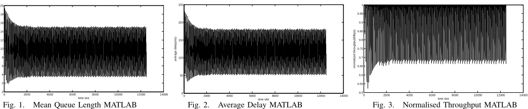
First the mean queue length is calculated and presented in figure 1.

The mean queue length in this figure is calculated by

P20

i=0iΠi in every slot. As we can observe in the figure, the

mean queue length of the model starts at zero, which represents the empty queue that the connection started with, then the mean queue length increases rapidly, which corresponds to the slow-start stage when the transmitting window size increases exponentially. If magnification is large enough, it can be observed that the mean queue length peaks at about the 50th time slot, when it almost reaches the maximal buffer size 20, before starting to decrease. This represents that it is most likely that the connection will transform into congestion avoidance at this time. In congestion avoidance stage, the TCP source increases and decreases the window size as it is receiving or missing acknowledgement for the packets that has been transmitted. As a result, the mean queue length also fluctuates

but ultimately within a relatively steady range. The average queue length of the entire duration of this experiment is 9.8147.

After the mean queue length of this experiment is calcu-lated from state distribution of the queue, the queueing delay is calculted and presented in figure 2.

In queueing theory performance modeling, delay or wait time of a customer in a queue is calculated with Little’s Result/Law using the mean queue length. As a result, these two are directly linked, so the result of the delay shares most of the features of the mean queue length process. Although delay is like second-hand data in this sense, it is much easier to be experienced and measured in a practical system, and it is also much easier to compare the value of delay calculated here with the delay value from NS-2 simulation later. The average delay for the connection is 121.1070ms.

Finally, throughput of this connection is calculated and presented in figure 3.

The throughput is another performance measurement that can be easily experienced and measured in a practical system, and it is relatively easy to be compared with simulation result as well. In queueing theory performance modeling, throughput is calculated by(1−Π0)β.(1−Π0)represents the probability

that the system is not empty, and in other words, the rate that the service is utilised. In these experiments, as a 100% utilised gateway represents a throughput of 1Mbps, the actually throughput of the connection can be calculated by(1−Π0)×

1M bps. The average throughput for the entire experiment is 0.9569Mbps.

It can be observed that this system represented by our model has a relatively high throughput, achieving at more than 96% of the maximal value, at the cost of a moderately high delay.

B. NS-2 Simulation Comparison

In this particular scenario, the topology of NS-2 simulation scenario is presented in figure 4.

(6)

0 10 20 30 40 50 60 0

2 4 6 8 10 12 14 16 18 20

experiment time(s)

queue length(packet)

Fig. 5. Instantaneous Queue Length NS-2

0 10 20 30 40 50 60 0

50 100 150 200 250

experiment time(s)

delay(ms)

Fig. 6. Instantaneous Delay NS-2

0 10 20 30 40 50 60 0

0.2 0.4 0.6 0.8 1.0 1.2

experiment time(s)

throughput(MB/s)

Fig. 7. Instantaneous Throughput NS-2

Fig. 4. NS-2 Topology

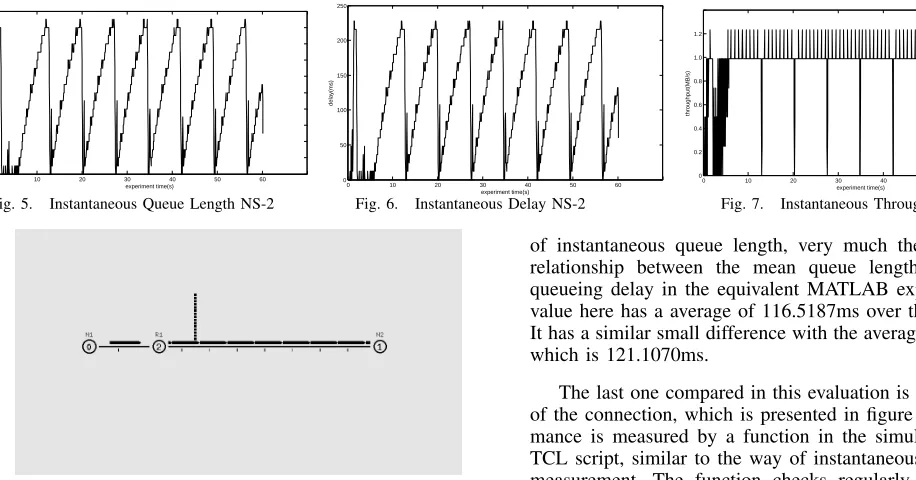
assumption in the MATLAB experiment. The queue in R1 utilises the drop-tail scheme, and the buffer size is 20 packets. All data packets in the simulation are 1500 bytes in size. The connection simulation runs for 60 seconds, and the queue length, queueing delay, throughput is captured through NS-2 build-in script functions.

The instantaneous queue length presented in figure 5 is captured through the queue monitor function in the NS-2 scenario TCL script. It checks the number of packets inside the queue of R1 frequently (in this case, every 0.05 second) and record the data into a file on the hard drive. It can be concluded that the TCP source behaved the way we expected. Because of the 20 packets maximal buffer size and the 1500 byte packet size, they represent 30000 byte in buffer which is smaller than the maximal window size of N1 - 65535 byte. As a result, the maximal window size will never be reached, and the connection will never reach a steady state. This figure may seem to look quite different than the MATLAB figure. The reason for this is because the queue length measured here is instantaneous queue length, and the one calculated in previous section is mean queue length, which can be considered as an average value of different instances of connection, or the performance of a connection duration a certain time period. The average queue length of this NS-2 experiment over 60 seconds is 9.7099 which is very close to MATLAB average of 9.8147.

The instantaneous delay of this TCP connection simulation is presented in figure 6. This value is captured by using the awk script to analyse the simulation trace file which contains every single event in the simulation. The script will locate the time stamps of every packet arriving at node R1, comparing them with the time stamps of they leaving node R1. Considering that the link speed is relatively low and the processing and transmitting delay is negligible, this time difference will be the instantaneous queueing delay at node R1 for each packet. Overall, the instantaneous delay share most of the property

of instantaneous queue length, very much the same as the relationship between the mean queue length and average queueing delay in the equivalent MATLAB experiment. This value here has a average of 116.5187ms over the 60 seconds. It has a similar small difference with the average in MATLAB which is 121.1070ms.

The last one compared in this evaluation is the throughput of the connection, which is presented in figure 7 This perfor-mance is measured by a function in the simulation scenario TCL script, similar to the way of instantaneous queue length measurement. The function checks regularly (in this case, every 0.05 second) how many packets have passed through the queue in question. Multiplied by the size of each packet, then the result is the throughput of the queue, and thus, the throughput of this connection. It is worth mentioning that while it may seem erroneous that some data point is above 1.2Mbps as the link capacity is only 1Mbps, this is because the way this value is calculated. Packets on both edges of the 0.05 time slot may be considered inside the slot while they are only partially inside, and the majority of them actually located in other time slot. This will cause certain slot to be considered with higher number of packets passing through, which causes the spike point in the figure. The average throughput value of the entire simulation of 60 seconds is 0.941Mbps, very similar to that of MATLAB calculation which has an average of 0.9569Mbps.

Generally speaking, this instance of NS-2 simulation has a very close performance measurements to the MATLAB calcu-lation of the model with equivalent parameters. The differences experienced here are considered to be the difference of a single instance over a statistical result which would hopefully be aleviated by performing more instances of simulation and calculation, and difference between TCP technical details of the TCP agent used in the NS-2 simulation and in the model, which would hopefully be aleviated as more accurate model being introduced in future research.

C. Evaluation with Different Parameters

(7)

10 20 30 40 0

5 10 15 20 25 30

buffer size

MATLAB NS−2

Fig. 8. Mean Queue Length and Buffer Size

10 20 30 40

50 100 150 200 250 300 350

buffer size

average delay(ms)

MATLAB NS−2

Fig. 9. Average Delay and Buffer Size

10 20 30 40

0.7 0.8 0.9 1 1.1

buffer size

average throughput(Mbps)

MATLAB NS−2

Fig. 10. Average Throughput and Buffer Size

1.5 2 2.5 3

9.4 9.5 9.6 9.7 9.8 9.9 10 10.1 10.2 10.3

arrival rate (Mbps)

MATLAB NS−2

Fig. 11. Mean Queue Length and Arrival Rate

1.5 2 2.5 3

114 116 118 120 122 124 126

arrival rate(Mbps)

average delay(ms)

MATLAB NS−2

Fig. 12. Average Delay and Arrival Rate

1.5 2 2.5 3

0.935 0.94 0.945 0.95 0.955 0.96 0.965 0.97 0.975 0.98

arrival rate(Mbps)

MATLAB NS−2

Fig. 13. Average Throughput and Arrival Rate

0.5 1 1.5

9.4 9.45 9.5 9.55 9.6 9.65 9.7 9.75 9.8 9.85

service rate(Mbps)

average queue length(packet)

MATLAB NS−2

Fig. 14. Mean Queue Length and Service Rate

0.5 1 1.5

115 116 117 118 119 120 121 122

service rate(Mbps)

average delay(ms)

MATLAB NS−2

Fig. 15. Average Delay and Service Rate

0.5 1 1.5

0.935 0.94 0.945 0.95 0.955 0.96 0.965 0.97 0.975 0.98

service rate(Mbps)

MATLAB NS−2

Fig. 16. Average Throughput and Service Rate

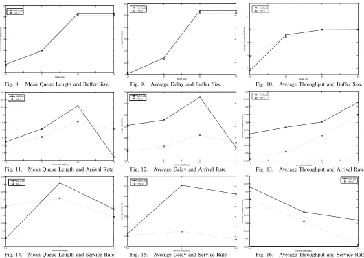
1) buffer size: In this group, the buffer size of the queue is changed between 10, 20, 30, 40, while all other parameters remain the same as in the previous 2 sections. The results are presented in figures 8, 9 and 10. When the buffer size varies, queue length is the first to be affected. It would be intuitive that when the maximal buffer size decreases, so will the average queue length, as the dropping event will happen much sooner for TCP source. Lower queue length means smaller queueing delay, but the queue are now more likely to be empty, so the service utilization will also decrease, and this is directly linked to the throughput, which will also decrease in this case. This can be observed from the first data sets of figures 8, 9 and 10.

When the buffer size increases, however, a similar conclu-sion may not be draw directly in reverse. In this case, because the maximal window size of the TCP source is 65535 byte, and the size of each packet is 1500 byte, which means there can be no more than 43 (65535₁₅₀₀ = 43.679) packets on the wire and buffer altogether even when the maximal window size reached. The result is when the buffer size is 30, the queue length will reach a stable value at 26. As there is no loss at all, the entire connection will be a steady flow of 1Mbps for about 59s of the simulation. It can be observed that the performance with buffer size 40 is almost exactly the same as buffer size 30.

Overall, the results from simulation and calculation match very well in all scenarios. The difference is slightly larger with the 10 buffer size set, as with the very small buffer size, the

difference between statistic calculation from queueing theory and deterministic simulation result become greater. It would be expected that if the buffer size is set to 2 (which is not very reasonable but still possible) this difference will become even greater. Difference is much smaller with 30 and 40 buffer size, as both of them reach a steady connection with very little dynamic behaviour.

2) arrival rate: In this group, the arrival rate (entering link bandwidth) is changed between 1.5Mbps, 2Mbps, 2.5Mbps, 3Mbps, while the buffer size and all other parameters remain as in the original experiment. The results are presented in figures 11, 12 and 13. The difference between all 4 data sets are not significant. Because the arrival rate is large enough relative to the service rate, and the queue length increases steadily at a moderate speed. The maximal buffer size is the same for all of these scenarios, which means their queue length are just different sets of linear increase from 0 to 20 then back to 0 at a slightly differed rate.

(8)

previous 2.5Mbps one, despite a considerably larger arrival rate. Overall, the 2 groups of data match quite well with each other, with it better on the lower arrival rate end. This is also because with the smaller difference between arrival rate and service rate, the queue length/window size will change slower, and thus the dynamic behaviour will be less significant.

3) departure rate: In this final group of experiments, the service rate (exiting link bandwidth) is changed between 0.5Mbps, 1Mbps, 1.5Mbps while all the other parameters remain the same as the previous sections, and the results are presented in figures 14 15 16. This group is essentially the same as the previous group with arrival rate, as in this type of queue only the relative value of arrival rate and service rate affects the performance of the queue. For example, two Geo/Geo/1/20 queues withα= 0.4, β= 0.2andα= 0.8, β= 0.4 has the same performance, as they can be potentially the model of exact same systems, but with different sizes of time slot. As a result, the increase of service rate shows the same result as an increase in arrival rate in reverse. The simulation and calculation results in this group match well with each other as well, so they further validate the proposed model and method.

V. CONCLUSIONS, LIMITATIONS ANDFUTUREWORK

In this paper, a new model with a traffic source mim-icking the AIMD behaviour of a TCP source is designed and demonstrated in detail. This model is able to represent the dynamic behaviour of a TCP source interacting with a bottleneck gateway, without using a single complicated source model. A mathematical interactive system between traffic source, gateway queue, and traffic destination (which responds to the incoming packets with acknowledgement) is developed, and is evaluated by performing MATLAB numerical solutions and comparing with an NS-2 simulation with equivalent pa-rameters.

This model system utilised a novel time-dependant queue-ing model calculation method for Geo/Geo/1/J queue, and is able to model a TCP connection behaviour in real time. In comparison, the traditional method ignore all stages of a flow where arrival rate is larger than the service rate, which is more than likely to happen in a practical network system. It waits for the system to reach the balance state if possible and performs any analysis based on that.

The model system has been evaluated quite extensively, with positive results. However, there are opportunities for future extensions and evaluations. For the major step of the ongoing extension, multiple TCP traffic sources will be con-sidered so that the model may better analyse practical network system. AQM schemes will also be included, and with the special calculation method introduced in this paper, in addition to the promising experiment results with the current drop-tail queueing system, useful studies, such as AQM dropping func-tion comparison, parameter optimisafunc-tion, can be performed.

REFERENCES

[1] L. Kleinrock,Queueing systems. Wiley-Interscience, 1975. [2] S. Stidham, “Analysis, design, and control of queueing systems,”

Operations Research, pp. 197–216, 2002.

[3] J. Artalejo and O. Hernndez-Lerma, “Performance analysis and optimal control of the geo/geo/c queue,” Performance Evaluation, pp. 15–39, 2003.

[4] Y. Xiong and Z. Bu, “Density evolution method for discrete feedback fractal m/m/1 traffic models,” in 2005 International Conference on Communications, Circuits and Systems, May 2005.

[5] S. W. Fuhrmann and R. B. Cooper, “Stochastic decompositions in the m/g/1 queue with generalized vacations,”Operations Research, pp. 1117–1129, 1985.

[6] J. hong Li and N. shuo Tian, “Analysis of the discrete time geo/geo/1 queue with single working vacation,”Quality Technology and Quanti-tative Management, pp. 77–89, 2008.

[7] I. Atencia and P. Moreno, “The discrete-time geo/geo/1 queue with negative customers and disasters,”Computers and Operations Research, pp. 1537–1548, 2004.

[8] D. G. Kendall, “Stochastic processes occurring in the theory of queues and their analysis by the method of the imbedded markov chain,”Annals of Mathematical Statistics, pp. 338–354, 1953.

[9] M. E. Woodward,Communication and computer networks: modelling with discrete-time queues. London Pentech, 1993.

[10] M. Hassan and R. Jain,High Performance TCP/IP Networking. Pear-son Education, 2004.

[11] L. Olawoyin, N. Faruk, and L. Akanbi, “Queue management in network performance analysis,” International Journal of Science and Technol-ogy, Dec. 2011.

[12] T. Szigeti and C. Hattingh,End-to-End QoS Network Design: Quality of Service in LANs, WANs, and VPNs. Cisco Press, Nov. 2004. [13] B. L. Granovsky and A. Zeifman, “Nonstationary queues: Estimation

of the rate of convergence,”Queueing Systems, pp. 363–388, 2004. [14] P. Leguesdron, J. Pellaumail, G. Rubino, and B. Sericola, “Transient

analysis of the m/m/1 queue,” Advances in Applied Probability, pp. 702–713, 1993.

[15] D. Worthington and A. Wall, “Using the discrete time modelling ap-proach to evaluate the time-dependent behaviour of queueing systems,” Journal of the Operational Research Society, pp. 777–788, 1999. [16] A. M. Mohammed and A. F. Agamy, “A survey on the common network

traffic sources models,” International Journal of Computer Networks (IJCN), pp. 103–115, 2011.

[17] D. Lee, B. E. Carpenter, and N. Brownlee, “Observations of udp to tcp ratio and port numbers,” inFifth International Conference on Internet Monitoring and Protection (ICIMP 2010), Barcelona, May 2010. [18] M. Hilbert and P. Lopez, “The worlds technological capacity to store,

communicate, and compute information,”Science, p. 60C65, Jun. 2011. [19] “Rfc: 793, transmission control protocol,”

http://www.ietf.org/rfc/rfc793.txt, September 1981.

[20] D. Bansal, H. Balakrishnan, S. Floyd, and S. Shenker, “Dynamic behav-ior of slowly-responsive congestion control algorithm,” inSIGCOMM, 2001.

[21] D. Katabi, M. Handley, and C. Rohrs, “Congestion control for high bandwidth-delay product networks,” inSIGCOMM, 2002, pp. 89–102. [22] “Rfc: 2581, tcp congestion control,” http://www.ietf.org/rfc/rfc2581.txt,

April 1999.

[23] “The network simulator - ns-2,” http://www.isi.edu/nsnam/ns/. [24] “Rfc: 6582, the newreno modification to tcp’s fast recovery algorithm,”