Energy Efficient Multi-Path Routing Algorithm Using Gray
System Theory for Improvement of Routing and Network
Stability in Internet of Things
Rogayye khaleghnasab1 . Karamolah Bagherifard1 . Samad Nejatian1 . Bahman Ravaei2
Abstract Internet of things (IoT) is a network of smart things. This indicates the ability of these physical things to transfer information with other physical things. The characteristics of these networks, such as topology dynamicity and energy constraint, challenges the routing problem in these networks. Previous routing methods could not achieve the required performance in this type of network. Therefore, developers of this network designed and developed specific methods in order to satisfy the requirements of these networks. One of the routing methods is utilization of multi-path protocols which send data to its destination using routes with separate links. One of such protocols is AOMDV routing protocol. In this paper, this method is improved using gray system theory which chooses the best paths used for separate routes to send packets. To do this, AOMDV packet format is altered and some fields are added to it so that energy criteria, link expiration time, and signal to noise ratio can also be considered while selecting the best route. The proposed method named RMPGST-IoT is introduced which chooses the routes with highest rank for concurrent transmission of data, using a specific routine based on the gray system theory. In order to evaluate and report the results, the proposed RMPGST-IoT method is compared to the ERGID and ADRM-IoT approaches with regard to throughput, packet receiving rate, packet loss rate, average remaining energy, and network lifetime. The results demonstrate the superior performance of the proposed RMPGST-IoT compared to the ERGID and ADRM-IoT approaches.
Keywords Internet of Things . Multi-Path Routing . Gray System Theory . Network Stability . RMPGST-IoT
1
Introduction
Recently, the demands of Internet of Things (IoT) keep growing. In the beginning, wireless sensor network (WSN) enables ubiquitous sensing technologies. As the WSN technology evolves, the proliferation and application of these sensing devices create the Internet of Things (IoT) [1, 2]. IoT is
Rogayye khaleghnasab [email protected]
Bahman Ravaei [email protected]
1 Department of Computer Engineering, Yasooj Branch, Islamic Azad University, Yasooj, Iran.
4 Department of Computer Engineering and Information Technology, Amirkabir University of Technology, Tehran, Iran
the next revolution, where the interconnection among smart objects creates an intelligent environment. It is estimated and expected to reach 24 billion IoT devices by 2020. As more and more IoT devices are connected and communicated, IoT applications generate tremendous IoT traffic. Since IoT traffic is for the communication between objects, the transmission reliability is critical, especially in a relatively unstable WSN, compared with wired network. We employ 500 sensor nodes distributed uniformly over the area of 3000∗3000m as seen in Fig. 1. A routing protocol decides how to send packets to other nodes. Routing protocols have two major divisions including Reactive and Proactive routing protocols. Routes are providing by the reactive protocols when it is needed. When it is necessary, control messages are transmitted by the path of data transfer, using these types of protocols. But, the needed time to find the route is increases. In addition, control messages are periodically exchanged by the proactive routing protocols immediately after start in order to search and propagate the routes. Local control messages together with messages across the entire network are sent by nodes to receive local nearby information and to share the structural information in all nodes of the network. In this research, we propose Multi-path routing protocol (IoT). The developed RMPGST-IoT protocol includes three key sections: a novel approach of distributed cluster discovery which can automatically establish local nodes, an innovative set of algorithms to adjust clusters and their head alternations based on the centralized position and isotropic energy propagation in all the sensing nodes, and a brilliant mechanism to reduce energy loss in long distance telecommunication.
Fig. 1 The devices deployed in IoT [3].
The paper presented here is organized as the following. Section 2 introduces some background terms regarding multi-path routing. In Sect. 3 brings the proposed RMPGST-IoT schema. Moreover, parameters utilised for performance evaluation are investigated and simulation results are discussed in Section 4. Finally, in Section 5, the paper is concluded.
2
Background terms
This section provides an introduction to the central concepts of this paper: multi-path routing, and detection schemes to provide protection for the IoT.
2.1Multi-path routing
paths will not affect the other ones. For transmitting a data packet between a source and a destination, it is possible to use any path of a multipath. Therefore, to get the most out of the data flow, and maximize share of the network bandwidth, the streams of data packets between a source and a destination can be divided between the paths [4].
2.2Detection schemes
In recent years, there have been many suggested researches on real-time routing protocols. And the central focus of them is divided into two main problems about multi-path routing protocols. The first one is the protocol requirement to guarantee the reliability of real-time packets in order to decrease the number of blank regions created by loss and delay. The other one is the protocol requirement to stabilize the energy loss of the network and avoid early expiration of some nodes.
MLB Method: In the IoT, large data transfers using wireless sensor networks has caused many problems. However, AODV routing stack in ZigBee protocol has no load balancing mechanism to handle corrupted traffic. Therefore, we develop multi-path load balancing (MLB) to replace AODV routing protocol in ZigBee. MLB is proposed for collaboration with ZigBee wireless network in the large scale. In this scenario, ZigBee is used as communication media in wireless sensor networks. In order to create a reliable ZigBee stack, ZigBee network layer is placed in MLB. MLB provides alternative routing service for ZigBee network without altering the existing stack in ZigBee. When a ZigBee router transmits the IoT data forward, MLB guides the ZigBee network layer in selecting the next hop with minimum load towards the IoT gate [3].
AOMDV Technique by means of SDN: In a research published by Kharkongo et al. in 2016, an AOMDV based routing protocol was suggested in which the power loss of heterogeneous devices has considered. Furthermore, An SDN controller is offered in the network which archives in an integrated style and creates a secure network by performing as an administrator that rejects access to selfish nodes in the network. The hypothesis of this study includes:
• The SDN controller is registered with devices
• There are different energy amounts for Heterogeneous devices • The overall network traffic is monitored by a centralized controller The stages of the suggested algorithm are listed below:
• Stage 1: The controller is registered with the nodes. The controller allocates an exclusive ID to every node in the network.
• Stage 2: The network is monitored by the controller.
• Stage 3: The source node discovers the information affecting the neighbour node. • Stage 4: Remained energy of the neighbourhood node is calculated.
• Stage 5: Based on the node energy, the source node transmits the packet. If the energy value is under the threshold value, the packet is sent. Else, other neighbour node is chosen.
• Stage 6: The controller will stop the selfish node by preventing it to add the network again. This study compares the AOMDV routing with SDN controller to other AODV routing protocols, DSR and DSDV. Achieved results with altered parameters determine that the suggested routing protocol has better performance than traditional routing protocols regarding to efficiency, packet delivery rate, and average end to end delay. Consequently, total performance of the network enhances using the suggested routing method [5].
criterion, takes into consideration the resource consumption of each node. Trust criterion increases the network lifetime. Topology criterion is aware of the node positions and enhances loading. Chanel health criterion, due to inappropriate channel conditions, protects the network against harmful attacks. Reputation criterion evaluates each of the participants of specific network operations for identification of specialized attacks. On the other hand, trust criterion, general adaptation, evaluates the fulfilment against hybrid attacks. SCOTRES has two types: one is embedded systems, and the other is real systems. The evaluations represented in this paper demonstrated that this system has the highest protection rate, while maintaining the performance for setting up real applications [6].
ERGID Method: A routing protocol called Emergency Response IoT based on Global Information Decision (ERGID) was suggested in the study of Qui et al. in 2016 to increase the reliability of data transmission performance and efficiency of the emergence response to IoT. Especially, in this study a mechanism called delay iterative method (DIM) which is founded on delay approximation was designed to answer the problem of disregarding valid routes. Additionally, a transfer plan called “Remaining Energy Probability Choice” (REPC) was recommended for balancing the network load together with focusing on the remained energy of the node. Consequences and examination of the simulation indicates that ERGID have better performance with respect to EA-SPEED and SPEED approaches regarding end to end delay, packet dissipation rate, and energy loss. Also, in this study some applied examinations were performed using STM32W108 sensing nodes. It was detected that ERGID can increase the network ability for real-time response [7].
AOMDV-IOT Technique: In this study, the suggested technique called AOMDV-IOT is introduced. It is a routing technique and up to the destination, it can perform as the router. The recommended method is not offered just for the node. The enhancements are mostly appropriate in IoT which is a unique technique for it. The principle object in this technique is detecting and generating effective connections between the nodes and the internet using the AOMDV routing protocol in the IoT. The internet connection table (ICT) is added in the suggested routing protocol to every node. Every node has two tables in this method including: routing table and ICT. ICT consists of four units: terminal node number, terminal node IP address, lifecycle, and hop value. Even though ICT uses extra memory, instead it can store connection counts and consequently decreases transmission delay. Comparison of AOMDV, simulating outcomes show that AOMDV-IOT has improved efficiency with respect to end to end delay, packet loss, and frequency in IoT. In this research, the multi-objective ad-hoc generated distance vector for the internet of things has been enhanced in such an approach that it can dynamically choose the direct internet transmission route by regular update of internet link table. Simulating effects show that while the AOMDV-IOT routing protocol rises the two routing packets, average end to end delay of the route falls [8].
to calculate the centralized location. Simulation results show that EECRP performs better that LEACH, LEACH-C, and GEEC. When the BS is in the network, EECRP can send a significant amount of data with very low energy loss. Therefore, network lifetime is longer for EECRP than it is for LEACH [9].
AOMDV method: A self-correcting path detection and information transferring route is suggested by AlZubi et al. for enabled applications in the Internet of Things (IoT). This routing procedure achieves at device level for self- restore and establishing its communication routes in a large-scale network. The routing practice is naturally opportunistic, need local device information instead of universal update. This opportunistic routing (OR) is built on best-fit traversing (BFT) algorithm to enhance the device availability in a precise way. The best-fit algorithm determines perfect neighbours for restarting interrupted communications in elongated mode [10].
Adaptive Distributed Routing Method: FANET networks are a key part of the IoT and can offer messaging facilities for various devices in the IoT and cyber-permitted applications. But, moving unmanned aerial vehicles (UAV) in FANETs creates random network link and increases complexity of routing algorithms for these applications, particularly in real-time routing. In this research, an effective opportunistic distributed routing technique is suggested to explain the above mentioned problem. For data transfer in this process, only the colleague nodes and local information are used by the transmitter. They maximize network use and preserve the end to end delay less than a stated threshold in order to care for variations of network and channel by designing and solving an optimization problem. Besides, they guess one stage delay for every communication of the transmitter node and use double parsing to alter the integrated problem into a distributed one. By this method, the transmitter nodes are only permitted to contact with local information and approximate delay in packet routs. Simulation outcomes indicate that the introduced routing technique enhances the network performance regarding its energy efficiency, quantity, and end to end delay [11].
REL Method: In the next work, Machado et al. proposed an energy and link quality-based routing protocol (REL) for IoT applications. In order to improve reliability and energy efficiency, REF selects an estimator mechanism based on the end to end link and the remaining energy. Furthermore, REL proposes an event-based mechanism to maintain load balance and prevent premature energy loss in nodes and the network. REF provides an end to end route selection plan based on cross-layer information with minimum overhead. In order to achieve energy efficiency, the nodes send their remaining energy to the neighbouring nodes. In this paper, route selection process is carried out using end to end link quality evaluation and optimal energy information. A new method is used for link quality estimation. REL utilizes the wireless link quality and the remaining energy while routing in order to increase system reliability and support QoS for IoT applications. REL uses a reactive pattern for discovering routes. This results in reduced signalling overhead and improved scaling capability. Route discovery process consists of diffusing RREQ and RREP messages. In large scale networks with high node density, results suggest that in REL, lifetime was improved up to %26.6, latency up to %17.9, and packet delivery up to %12 when compared to AODV and LABILE [12].
the routes. Moreover, NLEE algorithm guarantees better utilization of the energy available in the nodes. It also regularizes routing delay while discovering the shortest path in the network [13-18].
Table 1, summarizes the investigated efforts to design multi-path routing for IoT.
Table 1 Summary of the multi-path routing schema for IoT literature.
References Operation Advantages Disadvantages
MLB [3] Layer design and balancing load in order to create load balance and eliminate bottlenecks
Load balancing, decreased packet loss, and increased connections
Paying no attention to the remaining energy and lifetime of the node
[5] Routing in the internet of things based on the AOMDV protocol
Detecting malicious nodes and packet transfer based on the energy and improved network efficiency
Not taking into account other criteria such as distance etc. along the way of the packet SCOTRES
[6]
Secure routing with emphasis on energy consumption of the devices and decreasing it
Increased network lifetime while using trust criterion in order to prevent hybrid attacks
-
ERGID [7] Routing based on decisions made with general information
Improved data transfer performance and emergency response
The need to estimate delay in order to improve delay and network lifetime
AOMDV-IOT [8]
Discovering and establishing efficient link between nodes and the internet based on the AOMDV protocol
Decreased latency and decreased packet loss rate
More overhead because of storing two tables in each node and two extra routing packets
EECRP [9] Clustering algorithm while taking into account the energy criterion while routing and selecting the cluster heads
Distributed clustering and uniform load distribution among all of the sensor nodes
Not taking into account criteria other than energy while routing
ADRM-IoT [11]
Reducing the complexity of routing algorithms using distributed adaptive routing
Improved energy efficiency, throughput, and end to end latency
The need to carry out exact calculations to calculate delay
REL [12] Routing protocol based on link quality and energy
Improved reliability and energy efficiency
-
NLEE [13] Efficient energy protocol for improving energy efficiency in the internet of things
Improved latency – decreased power consumption
Overhead caused by counting the number of sent and control packets, hop count and remaining energy
3
The proposed RMPGST-IoT schema
In the following section, we design a RMPGST-IoT schema by employing the Gray System Theory algorithm. The proposed system consists of six steps, such as the assumptions applied in the proposed approach is discussed in Sect, 3.1. Adding new parameters to AOMDV is discussed in Sect, 3.2. Designing the routing packets in RMPGST-IoT is discussed in Sect. 3.3, Gray System Theory Steps is discussed in Sect. 3.4, Using gray theory in routingis discussed in Sect. 3.5, and the algorithm for the proposed RMPGST-IoT method is discussed in Sect. 3.6.
3.1The assumptions applied in the proposed RMPGST-IoT The assumptions Considered in the proposed approach include:
• Things existing in the network are not static; they should work independently.
• Each thing has limited energy and the initial energy of each thing is 𝐸𝑃𝑁where 𝐸𝑃𝑁 > 0. • Things gather data with a constant rate from the environment.
• Energy reduction and software issues can make a thing faulty.
3.2Adding new parameters to AOMDV
Because most of the devices are wireless, link stability fluctuation caused by movement or transfer medium characteristics in the internet of things affects the network performance. Efficiency of a dynamic routing protocol can be rated based on its ability to handle link unreliability and its computational and reconfiguration/rerouting overhead. Link stability as the basis of routing can lead to a protocol that has the following capabilities:
Movement Flexibility: Selected links are durable for longer periods of time against lost connections
in moving nodes.
Efficient Energy: Fewer disconnected links because of reduced rerouting, resulting in low connection
and computational overhead.
Stability: In order to reduce the overhead of the routing tables, more effective routes are stored longer.
We evaluate the link stability in our work with the energy, step count, signal to noise ratio, and route expiration time parameters corresponding to each route.
Signal to noise ratio is presented as SINR. The higher the SINRvalue is, the higher are the chances of
continuous connection and link for longer periods of time. The higher the remaining energy in a node, the higher are its chances of staying alive for longer periods of time and therefore the larger its transmission range. The higher the link expiration time (LET) and the lower the number of hops, the higher are the chances of the packets being delivered quickly and soundly.
Healthy node: the routes selected to transmit data must not be faulty.
In our proposed method, we estimate the link stability with the following factors: energy, hop count, Signal-to-Interference-Plus-Noise Ratio (SINR), and expiration time of each route. We also evaluate the healthy nodes with the following parameters: the message exchange rate in the transmitter circuit of the node and the fault of the node’s sensor circuit. However, it should be noted that a thing with very little energy or low signal-to-noise strength is faulty as well. The higher the SINR, the higher the probability of having more durable connections and links, and the lower the noise of sent data. In fact, the device transmitting data with high noise is not healthy and such data isn’t feed practically. On the other hand, the more the remaining energy of the thing, the higher the probability of its longer lifetime and the higher its transfer area. The next parameter is Link Expiration Time (LET) so that the longer LET leads to more durable link and the connection isn’t failed during data transferring. Also, the less the hop count parameter, the quicker the data transfer and the higher the probability of having a healthy package in the destination. In addition, when the message exchange rate in the transmitter circuit of the thing is high, it shows that this node is healthy and can communicate with objects around it and don’t eliminates data. The last parameter is the sensor circuit status that is calculated based on the measurement difference between a node and its neighbor node— the less the parameter, the better and healthier the node.
Signal to Noise Ratio: Noise ratio is defined as the ratio of the received signal (S) to a combination of noise strength (N) and interference (I). Definition of SINR is presented in Equation (1):
S SINR
N I
= +
(1)
SINRis estimated using the average reception during inactivity period. SINRis used to determine the quality of network links or connections.
Remaining Energy (Re): One of the most important elements while choosing a route is the remaining
lower their consumed energy, the more appropriate that route is to be selected. Remaining energy is calculated using Equation (2).
( ( ) ( ))
N N N
ER = EP t −ECo t (2)
In Eq. (2):
( ) ( ) ( ) : : N N N
ER t Remaining energy of the node
EP t Primary energy of the node
ECo t Consumed energy of the node
Hop Count (Hop): The Hop count parameter is the number of Hops between the origin node and the
destination node. The lower the Hop count of a route, the better that route is because less energy needs to be used in order to transmit the packet.
Link Expiration Time (LET): It is the amount of time for which the links stays stable. The longer
this time period is, the more stable the link between the nodes will be. This parameter depends on the movement speed of the nodes. The faster the nodes move, the more unstable the route between them will be and the sooner it will be destroyed. Link expiration time is calculated using Equation (3) based on the transmitted packets between the nodes.
In Eq. (3):
* cos * cos , ,
,
*sin *sin
i i j j
i j
i j
i i j j
a v v
b x x
d Y Y
C v v
= − = − = − = −
The nodes are aware of their location using GPS. In the above equation there are two nodes i and j
which are at (x yi, i) and (xj, yj) respectively. Their speeds are vi, vj and their movement angles are
i
and j. In the following section, details for each step are presented.
Message Exchange Rate (MER): in the transmitter circuit of the thing: the MER of a thing shows
that whether the thing is healthy or not. Also, the higher MER shows that the thing exchange message with its neighbors properly. The efficiency of the transmitter circuit of the thing 𝑃 is calculated as follows.
𝑃 = 𝑁
𝑇𝑡𝑖𝑚𝑒
(4)
Where 𝑁 is the number of received confirmation messages and 𝑇𝑡𝑖𝑚𝑒 indicates the time consumed in the network. The origin decides about the MER of a thing dependent on the volume of the test messages sent by the origin in that period. If the MER is low, the node is faulty otherwise, it is healthy.
Sensor Circuit Status (SCS): the SCS of a thing is detected by the thing itself. The thing 𝐼 calculates
the measurement difference between the 𝑘 (𝑘 = 1 … 𝑛) neighbor nodes. If measurement difference is less than the threshold (Δ𝑑𝑖𝑗 < 𝜃) then, Δ𝑑𝑖𝑗 = 0. The value of 𝜃 is dependent on the node density and can be different according to the application. In some cases, a high threshold may be needed to
2 2 2 2
2 2
( ) ( ) * ( )
( , ) ab cd a c R ad bc
LET i j
analyze the fault of the sensor circuit. The average difference of information 𝜃𝑖 is calculated as follows.
1 ... ... ...
i ij in
i
d d d
K
= + + + + +
(5)
If the value of the measurement difference is high, the node is faulty. When the measurement difference between a node and its neighbors is lower in a route, this route is better. The related steps are expressed in the following.
3.3Designing the routing packets in RMPGST-IoT
In the proposed method, all of the devices need to be equipped with GPS and have maximum initial energy. AOMDV routing packet format is expanded so that it can be used for RMPGST-IoT routing. This is achieved by adding new fields to AOMDV routing packets. RMPGST-IoT routing protocol, just like the base AOMDV protocol, has four packet formats. However, in the proposed RMPGST-IoT method, these formats are altered and required fields are added to these packets. Details of these packets are presented below.
HELLO Packet: This packet is used to discover neighboring devices in regular intervals. Adjacent
nodes exchange their location obtained through GPS and remaining energy information using HELLO packets. After exchanging the HELLO packet, each node updates its routing table and the remaining energy of neighboring nodes and also calculates SINRrate based on the received signal from the neighbor and link expiration time (LET) with the neighboring node based on its own location and the neighbor’s location and also writes them into its table.New format of theHELLOpacket is shown in Figure 2.
Fig. 2 New format of the HELLO packet.
RREQ Packet: The second packet is the route request (RREQ) packet. Each time a node tries to
communicate with other nodes in the network, route discovery process needs to be carried out. Therefore, the node broadcasts theRREQpacket publicly to find an appropriate route to its destination
RREQpackets consist of anIDto identify each packet, the destination IP address, sequence number, and network time stamp. Destination sequence number indicates the freshness of a route. We add the remaining node energy, SINRvalue, and the calculated LETwith the last hop based on theHELLO
message fields to theRREQpacket. Each node has calculated these parameters based on the Eq. (1) through Eq. (3) upon receiving theHELLOmessage and saved them in its table. Now, once theRREQ
message is received, each node on this route adds these information and transfers to the next node along the route to the destination.New format of theRREQpacket is shown in Figure 3.
Fig. 3 New format of theRREQpacket.
RREP Packet: The third packet is the route reply packet. After receiving the broadcastedRREQ
packets, many routes are discovered from the origin to the destination. Normally,RREPpacket
Unused Reserved
Packet type
Origin sequence number Origin IP address
Node energy Time stamp (origin time)
Node speed
Node location
Hop count Reserved
Packet type
Destination IP address RREQ public broadcast ID
Origin IP address Destination sequence number
Node remaining energy hop count
Accumulated route Time stamp
LET
consists of an ID to identify unique packets, origin IP address, sequence number, and accumulated routes. In the proposed method, we get the destination of everyRREQpacket from different routes and calculate the total number of hops, total remaining energy in each route, and totalSINRandLETin the links of each route and add them to the RREPpacket. Then, this packet is sent to the origin of that route. Therefore, we add the new total remaining energy of the route nodes, hop count, and total SINR
andLETfields to theRREPpacket.New format of theRREPpacket is shown in Figure 4.
Fig. 4 New format of theRREPpacket.
RERR Packet: Whenever a node discovers an error, it broadcasts a route error (RERR) packet with
the destination sequence number and infinite hop count. The origin node or any other node along the route can rebuild the route by sending a RREQpacket. If the origin node or any other node receives the RRERpacket, it needs to re-execute the route discovery process.
Test Packet:after detecting nodes, the origin sends a test message through all routes in the format
shown in figure 5 to take the responses of all the nodes in the routes. In this way, we can calculate two mentioned parameters namely MER and SCS.New format of theTestpacket is shown in Figure 5.
Fig. 5 New format of theTestpacket.
3.4Gray System Theory Steps
When units are evaluated using different parameters, some important parameters might be neglected. This happens specially when performance parameters have several values. Also, if the objectives and instructions of these parameters are different, results of analyzing them will be misleading. Therefore, performance evaluation parameters must be converted to a comparable sequence and therefore normalization is required. This is the gray relation creating step. In order to evaluate several devices, if m is the number of devices and n is the number of parameters, then the device number i will be described as Yi =
(
yi1,yi2,...,yij,...,yin)
where Yiis the value of parameter jfor devicei.i
Y can be converted to a comparable sequenceXi =
(
x xi1, i2,...,xij,...,xin)
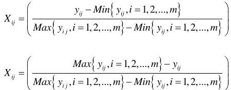
using Equation (6 ) and Equation(7). In other words, these parameters can be normalized using the presented equations.
, 1, 2,...,
, 1, 2,...,
, 1, 2,...,
ij ij
ij
i j ij
y Min y i m
X
Max y i m Min y i m
− = = = − = (6)
, 1, 2,...,
, 1, 2,..., , 1, 2,...,
ij ij
ij
i j ij
Max y i m y
X
Max y i m Min y i m
= − = = − = (7)
In Equation (6) and Equation (7), i and jare defined as follows:
1, 2,3,..., , 1, 2,3,...,
i n j m (8)
Hop count Reserved
Packet type
Destination IP address IDRREP
Origin IP address Origin sequence number
Time stamp Accumulated route
Total hop count along the route Total remaining energy of the nodes
along the route
Total LET along the route Total SINR along the route
Hop count Reserved
Packet type
IP address of Middle node Broadcasting ID the Test packet
Equation (6) is used for positive parameters. In this equation, the biggerXijis, the better the obtained results will be. In the proposed scheme, this equation is used for the remaining energy, link expiration time, and noise rate parameters. Equation (7) is used for negative parameters. In this equation, the smallerXijis, the better the results will be. This equation is used for the HOP count parameter. After creating the gray relations using the above equations, all of the performance values, just like normalized values, will be between zero and one. The closerXijis to one, the parameter will be more desirable. Therefore, the comparative series consisting of all ones will be the best choice. The target series is a series where all of the performance values are equal to one. Equation (9) illustrates the target series (X0) where all of its parameters are equal to one.
(
)
(
)
0 i1, i2,..., ji,..., in 1,1,...,1,...,1
X = x x x x = (9)
After this step, the main goal is finding a unit which is as close to this target series as possible. In order to find such a unit, gray coefficients must be calculated first. Steps to calculating this parameter are presented in the following section.
3.4.1 Gray Relation Coefficient
In the next step, gray relation value needs to be measured. This value is the gray relation rank. Calculating the gray relation rank requires the gray relation coefficient to be calculated first. Gray relation coefficient is used to determine the proximity ofXjiwithX0j. Equation (10) is used to calculate the gray coefficient.
(
)
min max0
max
,
j ij
ij
x x
+
=
+
(10)
In this equation,
(
x0j,xij)
is the gray coefficient and its value is betweenxji andxoj. In Equation (10), values of ij, min, andmaxare defined as Equation (11).
min
max
, 1, 2,..., ; 1, 2,...,
, 1, 2,..., ; 1, 2,...,
ij
ij
Min i m j n
Max i m j n
= = =
= = =
(11)
In these equations,ijis used to measure the difference betweenxijandxoj, while minis the minimum value among all of the parameters andmaxis the maximum value among all of the parameters. 𝜀 in Equation (10) is the detection coefficient which is a number in the
0, 1 interval. In most of the studies, 𝜀 is set to 0.5. After calculating the gray relation coefficient, gray relation rank is calculated for the aforementioned items. In the following section, how to calculate this rank is presented.3.4.2 Calculating the Gray Rank
Gray coefficient of two parameters is between zero and one in such a way that if this coefficient is one, it means that those two parameters are equivalent. On the other hand, if the coefficient is zero, those two parameters are independent. After calculating the gray coefficient, gray rank can be calculated using Equation (12) and use the resulting value in making various decisions.
(
0, i)
j*(
0j, ij)
In this equation, T X( 0,Xi)represents the gray relation betweenX0 andXi which demonstrates the
correlation between the reference sequence and the compared sequence.Wjis the weight or importance coefficient which is a parameter determined according to the problem structure. In our method, due to its higher importance, we have set the weight for the energy parameter higher than other parameters in the simulations. Equation (13) always holds for all theWj
1 1
n j j
W =
=
(13)In other words, according to the above equation, summation of all the weight values will be equal to one. Gray rank presents the similarity between the compared sequence and the reference sequence. The reference sequence for each evaluated unit represents the best possible performance which can be achieved using the compared sequence. This way, after the rank of every route has been determined according to their remaining energy, hop count, noise rate, and link expiration time parameters, the best route to the destination which has the best devices will be selected. This sequence is repeated until the decision-making process is completed. Because the final values are unities numbers between zero and one, overall rank of the route can be calculated according to the average gray rank of the mentioned parameters.
3.5Using Gray Theory in Routing
As mentioned in the previous sections, in this this research the quality of service, remaining energy level, noise rate (SINR), link expiration time, and hop count parameters are used to select the best route for efficient diffusion of information in the internet of things. Studies show that information diffusion using an efficient algorithm can significantly improve the performance of the internet of things. In this paper, several routes get selected for multi-path diffusion of information by checking the quality of service parameters of the devices (nodes). In other words, quality of service parameters of each node is used to select the best route for information diffusion. In related works, one or two quality of service parameters were used for information diffusion in the internet of things. The advantage of the proposed approach is the combination of different Quality of Service (QoS) parameters to select appropriate and faulty-node-free routes to disseminate data. Using several parameters to solve in deterministic optimization problems can lead to optimal or near-optimal solutions. However, it should be noted that using too many parameters can significantly increase the computational complexity and therefore decrease the network performance. The proposed RMPGST-IoT routing method for the internet of things consists of four steps. Neighbor discovery step, route discovery step, data transfer step, and detecting the health information of nodes. We will describe each step in the following sections.
3.5.1 Neighbor Discovery Step
3.5.2 Route Discovery Step
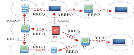
When the origin node decides to send a packet to the destination, it floods the network withRREQ packets to discover the suitable routes.RREQpacket includes the IP address of the origin and destination, sequence number, hop count, remaining energy in the node,LET,SINR, accumulated route, and time stamp. IP address of the origin and the destination are used to identify unique nodes in the network. The destination sequence number is used to show the suitable routes to the destination. Each node after receiving theRREQpacket, retrieves its neighbor information and inserts it into its routing table. Then inserts the new information along with its own information into theRREQpacket and sends it to the next node. Figure 6 demonstrates the flooding ofRREQpackets in the network in order to find routes leading to the destination.
Fig. 6 Flooding RREQ packets.
The destination node received multipleRREQpackets using different routes. Also, theRREPpacket includes the node ID to identify unique packets, destination IP address, sequence number, lifespan in the network, and accumulated routes. The accumulated routes are a list of separate routes from origin to destination. Moreover, three new fields, namely the totalLETof each route, totalSINR, and remaining energy of each route calculated by the destination node using theRREQpackets are added to theRREPpacket. After adding these fields, the destination node sends theRREPpacket using all of the routes and stores this information in its routing table. The origin node, upon receiving theRREPpackets from destination, stores the origin of these multiple routes in its routing table.
3.5.3 The step of discovering healthy information nodes
According to the Test messages sent by the origin node in that period, the origin node determines the MER of the node based on the equation 4. if the MER is low, the node is faulty, otherwise, it is healthy.
3.5.4 Data Transmission Step
After discovering several routes, the origin node calculates the total value of each parameter for all of the routes and saves them in a table. Table 2 is used to demonstrate the quality of service parameters for the nodes.
Table 2 Parameters of Quality of Service for each of the routes.
Parameters/Routes Total hop Count Total Time to Expiration of the Link Between the Nodes
Total Remaining Energy
TotalSINR
1 hop1 LET1 ERn1 SINR1
2
2 hop
LET2 ERn2 SINR2
n
n
hop
LETn ERnn SINRn
Now with the total value of the quality of service parameters for each of the routes to the destination known, gray relation theory is used to solve the problem. Since the abovementioned parameters have different units and therefore cannot be compared directly, a normalization method needs to be used to normalize the values and make them comparable. The normalization methods used in the gray theory are presented in Equation (4) and Equation (5). These equations have several applications. Equation (4) is used to normalize positive parameters while Equation (5) is used for normalization of negative parameters. In this research, three of the parameters are positive parameters which include the remaining energy, noise rate, and link expiration time. However, the hop count parameter is a negative one. In other words, the lower this parameter is, the better and therefore more desirable the final result will be. Therefore, Equation (4) is used to normalize the three positive parameters while Equation (5) is used to normalize the negative parameter. The values yielded after normalization using Equation (4) and Equation (5) for all of the parameters of the routes will be a scalar between zero and one. Value equal to one is the optimal condition and zero is the worst case. Therefore, one is considered as the reference series. As mentioned before, the reference series is presented as
(
)
(
)
0 i1, i2,..., ji,..., in 1,1,...,1,...,1
X = x x x x = where all of the normalized parameters are equal to one. After the most similar series to the reference series is determined for all of the nodes, the main goal is finding a route which is as close to the reference series as possible. Gray coefficient is used to find such a route. How to calculate the gray coefficient is presented in Equation (8). After determining the gray coefficient for all of the routes and their parameters, gray rank is used for ranking all of the routes based on the aforementioned quality of service parameters. How to calculate the gray rank using the parameters for the routes is presented in Equation (10) and Equation (11). The values resulted from this equation is a 1×n column matrix where n is the total number of available routes to the destination. This matrix consists of a decreasingly suitable sequence routes (based on the quality of service parameters) for information diffusion. The routes for multi-path routing of data are selected from the indices of the matrix with the highest gray rank values. These routes are saved in the table. This is repeated until the destination is changed or the route is eliminated.
values for each of the mentioned parameters are updated for every node and the above steps are repeated for the next information diffusion round.
Selecting the routs with proper QoS parameters i.e. high LET, SINR, energy, MSR, and SCS and less hop count to the destination improves the efficiency of the network and reduces its delay. However, in the proposed approach, we detect the faulty nodes in the routes and remove them from the network in addition to selecting the most appropriate routes for sending data. This is done in a separate phase by the origin and using fuzzy logic and previous information acquisition. Although the six considered parameters in the route selection step lead to selecting the best routes with the highest ranks by the origin, if there is a node with a faulty node among the selected routes, it will be removed from the route table.
3.5.5 Discovery of a faulty node employing fuzzy logic
In the proposed approach, we consider the four following parameters to detect the faulty nodes—SCS fault, MER fault, Battery level/remaining energy fault, and SINR value. These parameters are among the important criteria to detect the healthy and faulty nodes in the Internet of Things (IoT) network. The values of all the four parameters were calculated by the origin in the previous steps based on the control messages and Test message. In the following, we show how to use these parameters.
SCS fault: we declared that each node compares its measurement data with the measurement data of
its neighboring nodes using a test package. If the measurement difference of data doesn’t exceed the threshold, that node is considered a healthy node, otherwise, it is detected as a faulty node. In this way, if the value of the measurement difference linguistic variable is low, the sensor circuit of the node isn’t faulty. However, if the value is an average value, it is possible that a sensor circuit fault occurs after a time period.
MER fault: The origin decides about the MER fault of a node based on the rate of the Test messages
sent by the origin in that period. If the MER is low, the transmitter circuit of a node is faulty, otherwise, it is healthy.
Battery level/remaining energy fault: if the value of the remaining energy linguistic variable is low,
the battery fault occurs. if the battery level is intermediate, it will finish after a while and a battery fault can occur. Finally, if the battery level is high, the status of the battery is good.
SINR fault: SINR value is represented by fuzzy logic variables. If the value of the linguistic variable
id low, a noise fault occurs. if the value if intermediate, it shows that a noise fault will soon occur. Finally, if the SINR value is high, the status of the node is good and this node sends data properly.
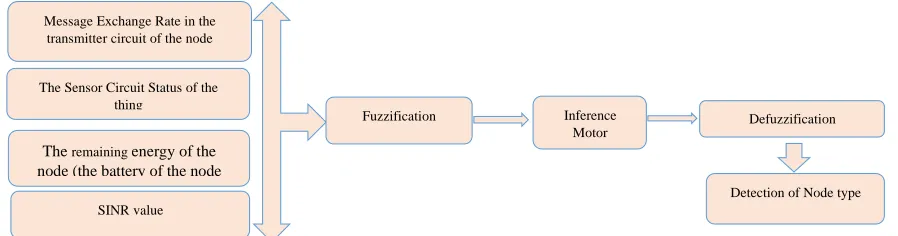
The hardware requirements of the things are evaluated by the fuzzy logic rules explained in the following. Figure 7 shows the fuzzy logic system with four input variables namely MER, SCS, Battery level fault, and noise fault.
Fig. 7 Fuzzy logic structure to detect the faulty nodes in the network Message Exchange Rate in the
transmitter circuit of the node
The remaining energy of the node (the battery of the node
SINR value
Fuzzification Inference Motor
Defuzzification The Sensor Circuit Status of the
thing
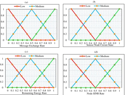
Three main processes in fuzzy logic are fuzzification, fuzzy inference, and defuzzification. In this section, the fuzzification phase is performed in the fuzzy logic system in which the numerical values are transformed into fuzzy values using fuzzy membership functions. As explained earlier, the inputs of fuzzy logic include MER fault in the transmitter circuit of the node, SCS fault, the remaining energy of the node, and the fault of existing noise in the sent message (SINR value). The linguistic set for the membership function of the fuzzy logic input parameters includes three defined values of low, intermediate, and high. The membership functions of MER fault in the transmitter circuit of the node, SCS fault, the remaining energy of the node, and SINR value are shown in the Figure 8.
Fig. 8 Fuzzy member function. (a) Message Exchange Rate in Circuit of Sender Node, (b) Sensor Node Circuit State, (c) Remaining Energy Rate, and (d) SINR.
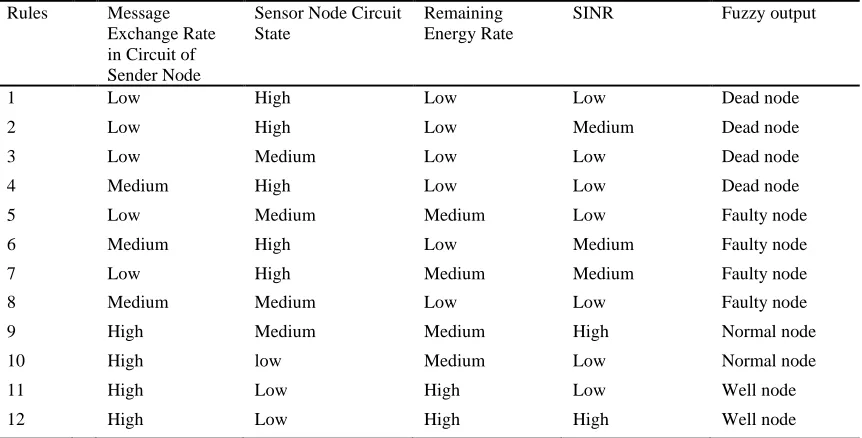
After determining the fuzzy logic input parameters, we performed the fuzzy inference phase and developed a rule set using expert knowledge. The fuzzy-rules-based knowledge is designed to integrate the input and output variables; this is done based on the criteria expressed by the origin. Since we have four criteria that each has three levels (low, intermediate, and high), we will have 64 (43) fuzzy rules in the knowledge base to design the fuzzy inference by the decision-making system. The fuzzy rules have been written based on the If-Then law. Every fuzzy rule includes an “If” term and a “Then” term. The “If” condition is made using predictions and a logical relationship is used to connect an input to the result. The “Then” term determines the degree of membership function and productivity. Some of these rules are presented in Table 3.
0 0.2 0.4 0.6 0.8 1
0 0.1 0.2 0.3 0.4 0.5 0.6 0.7 0.8 0.9 1 Message Exchange Rate
Low Medium
0 0.2 0.4 0.6 0.8 1
0 0.1 0.2 0.3 0.4 0.5 0.6 0.7 0.8 0.9 1 Sensor Node Circuit State
Low Medium
0 0.2 0.4 0.6 0.8 1
0 0.1 0.2 0.3 0.4 0.5 0.6 0.7 0.8 0.9 1 Remaining Energy Rate
Low Medium
0 0.2 0.4 0.6 0.8 1
0 0.1 0.2 0.3 0.4 0.5 0.6 0.7 0.8 0.9 1 Node SINR Rate
Low Medium
(a) (b
Table 3 Some of the fuzzy logic rules of the proposed RMPGST-IoT.
Rules Message Exchange Rate in Circuit of Sender Node
Sensor Node Circuit State
Remaining Energy Rate
SINR Fuzzy output
1 Low High Low Low Dead node
2 Low High Low Medium Dead node
3 Low Medium Low Low Dead node
4 Medium High Low Low Dead node
5 Low Medium Medium Low Faulty node
6 Medium High Low Medium Faulty node
7 Low High Medium Medium Faulty node
8 Medium Medium Low Low Faulty node
9 High Medium Medium High Normal node
10 High low Medium Low Normal node
11 High Low High Low Well node
12 High Low High High Well node
According to figure 9, the linguistic variables are organized in four ranges namely dead node, faulty node, normal node, and good node to determine whether a node is faulty or normal. A dead node is a node with an empty battery or a node which hasn’t responded to messages at all. A faulty node is a node which has low energy, responded to very few messages, have a significantly high measurement difference or a very weak signal. A normal node has an intermediate value of each criterion. Finally, a good node is a healthy node which has the maximum energy and responded to all messages with low noise, and low measurement difference.
Fig. 9 Fuzzy member function for fuzzy cost.
In the last phase, the results obtained in the two previous phases by the fuzzy system should be de-fuzzified in the defuzzification phase to make them understandable for the computer. In our proposed approach, we use the Centroid of Area (CoA) defuzzification method to defuzzify by equation (14) because the CoA defuzzification method has been widely used to defuzzify the Mamdani method.
( )
( )
A z
A z
x zdz
z dz
=
(14)
and faulty nodes in the network, the origin records the ID of these nodes and checks the routes selected in the previous step; in the case that a route contains such node, it will remove that node from the table. Then, it will disseminate the ID of the dead node to be eliminated from routing. After each round of data dissemination in the network, the values of the expressed parameters are updated for every node and the above-mentioned steps are repeated for the next round of the data dissemination. The data transfer process, route determination process, and faulty and dead node detection process in the proposed approach RMPGST-IoT are shown in the figures 10 and 11.
3.6The Algorithm for the Proposed RMPGST-IoT Method
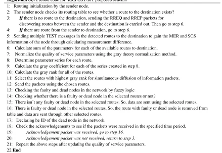
The overall steps of the algorithm for the proposed method based on the gray system theory for multi-path diffusion of information in the internet of things networks is as presented in figure 10. The proposed algorithm is repeated for each round of information diffusion after updating the quality of service parameters.
Fig. 10 Pseudo code of the proposed RMPGST-IoT method.
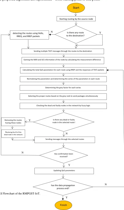
In the proposed RMPGST-IoT method, the traffic is distributed uniformly among the selected routes. This method guarantees that the energy of the nodes along the routes are used uniformly because the sender node will always select the routes with highest gray rank to ensure route reliability with regard to energy, link expiration time, MER, SCS, and also noise rate. In other words, the probability of the links being broken is reduced and therefore it is used more often than other routes. The proposed method also prevents the nodes from dying prematurely and the network being destroyed. The flowchart for the proposed RMPGST-IoT method is presented in figure 11. All of the steps to the proposed algorithm, from start to finish, can be found in this flowchart.The proposed approach avoids network collapse by detecting faulty and dead nodes and preventing using the routes having these
Algorithm (4): Pseudo code for RMPGST-IoT proposed schema 1: Routing initialization by the sender node.
2: The sender node checks its routing table to see whether a route to the destination exists? 3: If there is no route to the destination, sending the RREQ and RREP packets for
discovering routes between the sender and the destination is carried out. Then go to step 6. 4: If there are route from the sender to destination, go to step 6.
5: Sending multiple TEST messages in the detected routes to the destination to gain the MER and SCS information of the node through calculating measurement difference.
6: Calculate sum of the parameters for each of the available routes to destination.
7: Normalize the quality of service parameters using the gray theory normalization method. 8: Determine parameter series for each route.
9: Calculate the gray coefficient for each of the series created in step 8. 10: Calculate the gray rank for all of the routes.
11: Select the routes with highest gray rank for simultaneous diffusion of information packets. 12: Send the packets using the chosen routes.
13: Checking the faulty and dead nodes in the network by fuzzy logic
14: Checking whether there is a faulty or dead node in the selected routes or not?
15: There isn’t any faulty or dead node in the selected routes. So, data are sent using the selected routes. 16: There is faulty or dead node in the selected routes. So, the route with faulty or dead node is removed from table and data are sent through other selected routes.
17: Declaring he ID of the dead node in the network.
18: Check the acknowledgements to see if the packets were received in the specified time period. 19: Acknowledgement packet was received, go to step 16.
nodes. The flowchart of the proposed approach RMPGST-IoT is shown in figure 11 in which all steps of the proposed algorithm are represented—from starting point to end point.
Fig. 11 Flowchart of the RMPGST-IoT.
N
Y Y N
N Y
N Y
Is there any dead or faulty node in the selected route?
Updating QoS parameters
Start
Starting routing by the source node
Is there any route to the destination?
Sending multiple TEST messages through the routes to the destination
Calculating the total QoS parameters for each route using RREP and the responses of TEST packets
Selecting the proper routes based on the grey rank to send packages simultaneously
Sending messages through the selected routes
Has confirmation been received?
Finish detecting the routes using Hello,
RREQ, and RREP packets
Normalizing the parameters and determining the series of the parameters in each route
Determining the grey factor for each series
has the data propagation process end?
Gaining the MER and SCS information of the node by calculating the measurement difference
Checking the dead and faulty nodes in the network by fuzzy logic
Removing the routes having these nodes
4
Evaluating the Performance
In the following section, the performance of our proposed RMPGST-IoT approach is evaluated to multi-path routing problem.
5.1Performance metrics
In this section, the effectiveness and performance of our proposed RMPGST-IoT approach is thoroughly evaluated with comprehensive simulations. The results are compared with ERGID and
ADRM-IoT approaches proposed in [7] and [11], respectively. The throughput, packet receiving rate, packet loss rate, average remaining energy, and network lifetime are evaluated. Notations utilised here are listed in Table 4.
5.1.1 Average Throughput
Average throughput is the division of the sum of packets sizes received at the destination sensor node, to the difference of simulation stop and start time [19]. Eq. (15) obtains the average throughput for N experiments, and is calculated in Kilobits per second.
1 * 1 8 _ * * 1000 N i s i p T X P AT
N S S
= = −
(15)5.1.2 Packet Receiving Rate
PRRis the division of the total data packets received at the destination thing, to the total number of data packets transmitted by the source thing, described in percentage [20-24]. The averagePRR
obtained for N experiments is demonstrated by Eq. (16).
1 1 1 * *100 N i i N i i X PRR N Y = = =
(16)5.1.3 Packet Loss rate
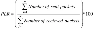
PLR occurs when one or more packets of data traveling across a computer network fail to reach their destination.PLRis typically caused by network congestion. Packet loss is measured as a
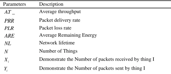
Table 4 Abbreviated notations Parameters Description _
AT Average throughput
PRR Packet delivery rate
PLR Packet loss rate
ARE Average Remaining Energy
NL Network lifetime
N Number of Things
i
X Demonstrate the Number of packets received by thing I
i
percentage of packets lost with respect to packets sent. The lower value of the packet loss means the better performance of the protocol. The PLRis calculated in Equation (17) follows:
1 1 *100 N j N j
Number of sent packets PLR
Number of recieved packets
= = =
(17)5.1.4 Average Remaining Energy
As demonstrated in Eq. (15), unconsumed energy in the node in an arbitrary time instance is the excessive energy maintained in the node following a concluded communication with the receiver. Examples of remaining energies are the energy for transmission, energy for reception, wasted energy in the system (Esys), fading effects, etc. The parameters exploited for theAREare listed in Table 4.
Table 4 Parameters used for average residual energy
Parameters Description
0
di Reference distance larger than the Fraunhofer-distance
di The distance on which the packet is transmitted
Lb demonstrates the number of bits per packet (BPP)
2
di Refers to the power loss of free space channel model
4
di Power loss of multi-path fading channel model
elec
E Amount of energy getting dissipated during transmission or reception
lbfsi Transmission efficiency
lbmpi Condition of the channel
residual initial X X sys
Energy =Energy − ET +ER +E Where (18)
2 0 4 0(1 , ) ,
,
X elec fs
elec mpi
ET b di lbE lb di di di
lbE lb di di di
= +
= +
(19)
Energy consumed during packet transmission ETX(1 ,b di)and packet reception (ERX ) are calculated using Eq. (18), and Eq. (19), respectively.
.
X elec
ER =lbE (20)
Simulated parameter is set as: 2
4 100 / , 20 / / ,
0.0015 / /
elec
fsi
mpi
E nJ bit
pJ bit m
pJ bit m = = =
Ifdidi0, multipath fading effect occurs, and energy is wasted during transmission. However, since the fading scheme is out of the scope of this paper, the distance is considered to be lesser than the Fraunhofers distance. Moreover, the information for channel state is not considered, while transmission efficiency is considered to be 1.
5.1.5 Network Lifetime
communication with the receiver is the life time aggregate for all the mentioned nodes at any time instance. If the network is clustered, the network lifetime is the total lifetime for all things [25-32]. Eq. (21) demonstrated the calculation of the NLvalue.
1 m
i i
NL Things
=
=
Where Thingsiis the lifetime of 𝑖 th things. (21)5.2Simulation setup and comparing algorithms
The difficulties in implementation and debugging IoTs in real networks, raises the necessity to consider simulations as a fundamental design tool. The main advantage of simulation is simplifying analysis and protocol verification, mainly in large-scale systems. In this section, the performance of our proposed approach is evaluated using NS-3 as the simulation tool, and the results are discussed further. It is worth mentioning that all RMPGST-IoT, ERGID and ADRM-IoT parameters and settings are considered to be equal.
5.3Simulation results and Analysis
In this section, we analyze the performance of RMPGST-IoT under the two scenarios (described in Table 5). There are 500 IoT things uniformly deployed in the network area initially. Some important parameters are listed in Table 5.
Table 5 Setting of simulation parameters. Parameters Value
Coverage area (m x m) 3000 x 3000
Simulation tool NS-3
MAC layer protocol IEEE 802.11
Transport UDP/IPv6
Communication range of each node 300 m
Channel bandwidth 3 Mbps
Traffic type, rate CBR, 10 packets/sec
Mobility model Random way point
RX and TX ratio 90%
Number of things, and Packet size 500, 256 Kbps Number of connections, and Pause time 50, 100 sec Maximum mobility (varying) 5 m/sec - 25 m/sec
Simulation time (in Sec) 500-2000
Table 6-10compares the performance of RMPGST-IoT with that of ERGID and ADRM-IoT in terms of throughput, packet receiving rate, end to end delay, average residual energy, and network lifetime.
Table 6 AT_ (in Kbps) of various frameworks with varying degree of rate of transmission (kb/s).
Rate of Transmission (kb/s) Average throughput (Kbps)
ADRM−IoT ERGID RMPGST−IoT
10 610 1060 1440
15 730 1207 1600
20 1108 1480 2005
25 1380 1670 2440
30 1604 1790 2700
35 1803 1900 3000
Table 7 PRR (in %) of various frameworks with varying degree of rate of transmission (kb/s).
Rate of Transmission (kb/s) PRR (%)
ADRM−IoT ERGID RMPGST−IoT
10 68.23 77.4 84.4
15 70.13 80.1 86.4
20 74.2 82.9 89.6
25 75.4 86.3 90.1
30 78.3 87.4 92.4
35 81.1 89.3 95.3
40 83.9 91.7 97.4
Table 9 ARE (in Joule) of various frameworks with varying degree of rate of transmission (kb/s).
Rate of Transmission (kb/s) ARE (Joule)
ADRM−IoT ERGID RMPGST−IoT
10 720 850 1004
15 710 812 940
20 640 800 840
25 601 750 810
30 580 743 804
35 532 731 790
40 491 690 770
Table 10 NL (in Sec) of various frameworks with varying degree of rate of transmission (kb/s).
Rate of Transmission (kb/s) NL (Sec)
ADRM−IoT ERGID RMPGST−IoT
10 490 680 900
15 401 610 790
20 335 550 730
25 306 495 697
30 295 415 660
35 250 330 615
40 220 318 604
Average throughput: Figure 12 shows the comparison of the RMPGST-IoT proposed scheme, ERGID and ADRM-IoT models in term of AT_. (a) Number of Things, (b) Simulation time, (c) Speeds, and (d) Number of CBR sources respectively. As shown in the diagrams, the proposed method outperforms the ERGID and ADRM-IoT methods with regard to throughput as well. On the basis of the results of Figure 12, theAT_of RMPGST-IoT is 2630 Kbps, ERGID is 2135 Kbps, and ADRM-IoT is 1340 Kbps. This is due to the fact that RMPGST-IoT selects routes on the basis of gray system theory information, with end-to-end link quality estimation (QoS-aware), unlike ERGID and ADRM-IoT models that only chooses paths based on Global Information Decision (GID).
Table 8 PLR (in %) of various frameworks with varying degree of rate of transmission (kb/s).
Rate of Transmission (kb/s) PLR (%)
ADRM−IoT ERGID RMPGST−IoT
10 31.3 22.1 14.3
15 29.3 20.3 13.2
20 23.5 17.3 10.2
25 22.4 13.2 9.3
30 18.5 12.1 8.1
35 16.3 10.3 4.3
Fig. 12 Comparison of the RMPGST-IoT proposed scheme, ERGID and ADRM-IoT approaches in term of Throughput. (a) Number of Things, (b) Simulation times, (c) Speeds, and (d) Number of CBR sources.
Figure 13 shows the relationship PRR and (a) Number of Things, (b) Simulation time, (c) Speeds, and (d) Number of CBR sources respectively. As seen in figure 13, the proposed method in this paper (RMPGST-IoT) has better PRR than ERGID and ADRM-IoT. This is because in the proposed method, packet routing is done through the routes with high remaining energy, link expiration time, and signal to noise ratio. Also, there are two reasons for achieving high PRR, stabled routes sustaining over a long period of time are identified in the route discovery plane and the replication is curtailed in the successive plane.This ensures improved message transfer in a unique manner over the same link, increasing the PRR. It exhibits a high-level of performance with a high PRR (more than 95.34%) as compared to ERGID and ADRM-IoT approaches.
Fig. 13 Comparison of the RMPGST-IoT proposed scheme, ERGID and ADRM-IoT approaches in term of PRR. (a) Number of Things, (b) Simulation time, (c) Speeds, and (d) Number of CBR sources.
(a) (b)
(d) (c)
Fig. 14 shows the average packet loss ratio (PLR) against (a) Number of Things, (b) Simulation time, (c) Speeds, and (d) Number of CBR sources for all the simulated approaches. When the 54, 67, 22 node come to failure, the PLR of the RMPGST-IoT protocol is 13.5%, which is better than the ERGID and ADRM-IoT. The reason behind the better performance of RMPGST-IoT is, it because it reacts more precisely to congestion than other protocols.
‘
Fig. 14 Comparison of the RMPGST-IoT proposed scheme, ERGID and ADRM-IoT approaches in term of PLR. (a) Number of Things, (b) Simulation time, (c) Speeds, and (d) Number of CBR sources.
Figure 15 shows the comparison of the RMPGST-IoT proposed scheme, ERGID and ADRM-IoT models in term of ARE. (a) Number of Things, (b) Simulation time, (c) Speeds, and (d) Number of CBR sources respectively. This criterion presents theAREin the nodes after routing has been carried out and is calculated using equation 13 which is calculated by subtracting the consumed energy from the initial energy. As seen in figure 15, theAREin the nodes is calculated at 100 and 1000 seconds in every simulation. The simulation results present that theAREin the nodes for the proposed RMPGST-IoT is higher than the ERGID and ADRM-RMPGST-IoT methods. This is because in the proposed method, routing is carried out using routes which consist of nodes which are better than the nodes in other routes with respect to hop count, noise rate,ARE, and link expiration time criteria. Therefore, taking into account the hop count criterion leads to lower energy consumption, while selecting the route which consists of nodes with higher energy levels controls the network energy and increases the ARE . Therefore, the RMPGST-IoT performs better in this regard as well. TheAREin RMPGST-IoT, ERGID and ADRM-IoT algorithms is reduced by 700, 600 and 470%, respectively, while the number of things is increased by 940, 690 and 550%, respectively.
(d) (c)
Fig. 15 Comparison of the RMPGST-IoT proposed scheme, ERGID
![Fig. 1 The devices deployed in IoT [3].](https://thumb-us.123doks.com/thumbv2/123dok_us/1016505.1601608/2.612.307.540.326.459/fig-devices-deployed-iot.webp)