NIR model development and robustness in prediction of melon fruit total soluble solids
8
0
0
Full text
(2) 2. Australian Journal of Agricultural Research. (no s.d. reported) with “no bias errors”, whereas Colour Vision Systems claim a RMSEP of <1%. The Sumitomo product appears to be no longer commercially offered. The demise of this product may reflect the high price of the equipment (approx. $AUD 1 000 000 for a single-lane pack line incorporating the NIR sensor) or equipment instability problems (laser output instability, temperature control). The above manuscripts (and commercial product literature) focus on reporting calibration model statistics or a prediction of a subset of the population from which the calibration population is drawn. Model performance in validation of new populations, not included in the calibration population, is a harsher exercise. Equipment manufacturers appear to rely on frequent recalibration to address this issue, with the exception of the Sumitomo laser unit, which was marketed on the basis of calibration model stability. Model updating is practiced in a wide range of NIR application areas, generally involving selection of representative samples of the new population for addition to the calibration population (e.g. Peiris et al. 1998; McGlone et al. 2003). For further review, see Guthrie et al. (2005a). In a previous exercise with mandarins (Guthrie et al. 2005b), it was demonstrated that model updating following addition to the calibration population of a relatively small number of samples (<20), chosen by any procedure (e.g. random) from the validation population, was a successful strategy. Model robustness across populations of fruit has been noted to be sensitive to changes in growing conditions and variety (McGlone and Kawano 1998; Peiris et al. 1998). In Guthrie et al. (2005b), model performance for prediction of intact mandarin TSS was shown to be more sensitive to year than to time within a growing season or growing location. In melon, Ito et al. (1999) noted that individual varietal calibration models are successful when predicting Brix on the same variety within the same season. He reported on the use of a calibration model developed in 1 season to predict a single lot from the subsequent season. The only published work on TSS model robustness in intact melons across multiple populations, varieties, and seasons is that of Guthrie et al. (1998). In this work, stepwise multiple linear regression (MLR) models were developed using 3–5 wavelengths, rather than modified partial least squares (MPLS) regression of the full spectrum, from reflectance spectra. Model performance was reasonable across some, but not all, varieties, and model performance markedly deteriorated across populations of the same varieties harvested at different times within a season. The reflectance technique is likely to optically sample the fruit to a depth of approximately 5 mm only (e.g. Lammertyn et al. 2000). The low coefficient of determination for the calibration population (Rc 2 ), coefficient of determination of the validation population (Rv 2 ), and higher RMSEP obtained for particular varieties (e.g. Eastern Star and El Dorado) were attributed to the nature of the skin (irregular and thicker epidermal layers) of these varieties. Further, as there. J. A. Guthrie et al.. is a poor correlation between skin and inner mesocarp TSS, Guthrie et al. (1998) suggested that the correlation of mesocarp TSS with spectral data may represent a secondary correlation with another constituent of the skin and green flesh layers. A breakdown in this secondary correlation could be responsible for the lack of model robustness. Sugiyama (1999) reported that absorbance at 676 nm was closely correlated with TSS, and used this character in imaging of TSS distributed across the cut melon surface. Absorbance at 676 nm presumably acts as an index of chlorophyll content, with TSS related to chlorophyll content indirectly, through fruit maturity. However, these models predicted poorly across different varieties, and subsequent work focussed on the use of spectroscopically justified wavelengths involving the use of the second derivative at 880 and 910 nm (Tsuta et al. 2002). In this manuscript we further examine the issue of rockmelon TSS model robustness, and the use of model updating procedures using small numbers of samples from the new population. Thus this work extends the consideration of Guthrie et al. (1998), using the partial transmittance instrumentation characterised in Walsh et al. (2000), and the model updating procedure described for mandarins in Guthrie et al. (2005b). Materials and methods Plant material Rockmelon fruit (Cucumis melo L.) varieties Eastern Star, Hammersley, Doubloon, Highline, Malibu, Mission, El Dorado, Colusa, Sterling, and Hotshot were obtained after commercial harvest from growers in 4 growing districts [Bundaberg (24.9◦ S, 152.3◦ E), Chinchilla (26.5◦ S, 150.4◦ E), Gumlu (19.9◦ S, 147.7◦ E), and Kununurra (15.5◦ S, 128.4◦ E)]. In all, 22 populations of various varieties of rockmelons (each of approx. 100 fruits) obtained over different seasons and growing districts, were used for spectral acquisition and then assessed for TSS. A spectrum was collected per fruit from the equatorial region (defined relative to the stem–calyx axis) and the area scanned was then excised from the fruit (60-mm-diam. core to a depth of 20 mm), skin removed, crushed to extract the juice, and the TSS assessed using digital refractometry (Bellingham and Stanley RMF 320). All populations were alphabetically named within each year. Five rockmelon fruits (variety Doubloon) were assessed for TSS distribution within the mesocarp. Twelve slices, each of approximately 1-cm thickness, were taken from the distal (calyx) end through to the proximal (stem) end of each fruit. Twelve TSS measurements per slice (6 from the outer and 6 from the inner mesocarp) were made, with sampling at and between each of the 3 vascular tissue areas. Outer mesocarp was defined as 0–20 mm in depth and inner mesocarp as from 20 mm to the seed cavity. Data were normalised to the TSS concentration at slice 6 (equatorial) of the inner mesocarp. The penetration of near infrared radiation through an intact fruit was visualised by illuminating 1 side of the fruit equator with a 100-Watt halogen lamp and monitoring 180◦ to this point with a Zeiss MMS1 spectrometer. The fibre optic bundle of the MMS1 was moved over a grid pattern, detecting light at the wavelength of maximum detected intensity (820 nm) from a 1-cm2 area of the fruit flesh surface as the fruit was consecutively cut away in 1-cm thicknesses from the opposite end to the light source (in the plane perpendicular to the lamp–fruit axis). The results of the light penetration were plotted in a volumetric-data visualisation software package (Slicer Dicer ver. 3.0)..
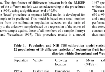
(3) NIR prediction of melon total soluble solids. Australian Journal of Agricultural Research. Spectral acquisition Spectra were collected over the wavelength range 306–1130 nm using a NIR-enhanced Zeiss MMS1 spectrometer (photo-diode array, comprising 256 silicon detectors with a resolution of approx. 3.3 nm) and 4 tungsten halogen lamps of 50 Watt each, in a partial transmission optical configuration as described in Walsh et al. (2000) (45◦ angle between illumination source and detector, relative to the fruit centre, with the detector probe in contact with the fruit surface). White (Teflon tile) and dark reference measurements were taken at the start of each experimental run. Spectra were averaged over 4 scans at an integration time of 200 ms per scan. Chemometrics The software package WINISI (ver. 1.04a) (ISI International, USA) was used for all chemometric analysis. WINISI uses a modified partial least squares regression (MPLS) procedure in which the reference data and the spectral data at all wavelengths are scaled to give a standard deviation of 1.0 before calculation of each subsequent MPLS factor (Shenk and Westerhaus 1991). Calibrations were developed using MPLS in both ‘global’ and ‘local’ WINISI procedures (based on the combined year 1998 and year 1999 populations). In the ‘global’ procedure a single MPLS calibration model is developed using all samples in the calibration population (excluding ‘outliers’). The ‘global’ WINISI models were optimised in terms of wavelength interval, derivative condition, and scatter correction technique. The significance of differences between both the RMSEP and bias of the different models was tested according to the procedures of Fearn (1996), using a significance level of 95%. In the ‘local’ procedure, a separate MPLS model is developed for every sample to be predicted. This model is based on a small number of spectra from the calibration population selected on the basis of similarity to the unknown sample (based on a regression of the scores of the unknown sample against those of all members of a sample library) (Shenk and Westerhaus 1997). This procedure results in a model. ‘over-fitted’ in the sense that the model is fit only for use in prediction of 1 unknown sample. The number of samples used (20–100, steps of 20), the number of MPLS factors used (5–25, steps of 5), and the number of MPLS factors removed (1–5, step of 1) (125 combinations) were optimised on the basis of lowest RMSEP(C) for validation across the 5 populations from the year 2000 (as used in Table 1) (data not shown). The WINISI software forced the removal of at least 1 MPLS factor, on the basis that the first MPLS factor is indicative of the scattering of light in the sample due to particle size and not the attribute of interest. Calibration performance for both ‘local’ and ‘global’ MPLS procedures was assessed in terms of Rv 2 , RMSEP, standard deviation ratio (SDR = s.d./RMSECV or RMSEP), slope, and bias of the validation populations as per Guthrie et al. (2005a). The SDR statistic facilitates comparison of different populations with differing s.d.s. The best data pre-treatment (second derivative with gap size of 4 data points either side and no scatter correction, data not shown) was used in all subsequent model development. The RMSECV, RMSEP, and bias values were tested for significance (P = 0.05) using the procedure of Fearn (1996). In a separate exercise, the effect of spectral window on partial least squares (PLS) calibration model performance for TSS was optimised in terms of root mean squared error of calibration (RMSEC) using a moving PLS interval algorithm, developed in Matlab (ver. 7.0) – PLS toolbox (ver. 3.5 by Eigenvector) (Guthrie et al. 2005a). The combined populations of years 1 and 2 (17 populations comprising 1467 spectra) were used, with second-derivative (WINISI gap size 4 without scatter correction) absorbance data interpolated to 3-nm steps. The start and end wavelengths of the spectral window were varied from 650 to 950 nm, and 750 to 1050 nm, respectively, in increments of 3 nm, and a map produced that involved 20 200 separate PLS models. Model performance is reported in terms of RMSEC rather than RMSECV in this exercise. In these iterations the number of PLS factors was kept constant to allow a direct comparison of the different spectral windows, thus making the use of RMSECV obsolete.. Table 1. Population and NIR TSS calibration model statistics using MPLS ‘global’ procedure for 22 populations of 10 different varieties of rockmelon fruit harvested over 3 years and from 4 growing districts within Queensland and Western Australia Population. Variety. Growing location. 1998a 1998b 1999a 1999b 1999c 1999d 1999e 1999f 1999g 1999h 1999i 1999j 1999k 1999l 1999m 1999n 1999o 2000a 2000b 2000c 2000d 2000e. Eastern star Hammersley Eastern star Eastern star Eastern star Eastern star Eastern star Hammersley Doubloon Doubloon Doubloon Doubloon Highline Malibu Mission El dorado El dorado Colusa Sterling Hotshot Hotshot Hotshot. Bundaberg Chinchilla Gumlu Gumlu Gumlu Gumlu Gumlu Gumlu Chinchilla Chinchilla Chinchilla Chinchilla Chinchilla Chinchilla Gumlu Gumlu Gumlu Kununurra Kununurra Gumlu Kununurra Kununurra. 3. n. Mean (%TSS). s.d.. # MPLS factors. Rc 2. RMSECV (% TSS). SDR. 75 80 71 80 90 78 100 80 85 86 99 99 90 92 105 130 100 100 96 80 100 99. 8.0 7.5 9.0 9.4 8.9 9.7 9.3 7.6 8.6 8.3 7.6 8.5 8.8 7.5 9.9 11.8 9.4 9.3 9.3 8.3 10.3 9.5. 1.42 1.16 1.10 0.93 1.03 0.95 1.91 1.12 1.37 1.25 0.93 1.03 1.10 1.01 1.10 1.66 1.70 1.80 0.88 1.32 1.00 0.95. 7 8 6 8 8 6 9 7 6 7 13 8 7 8 7 7 7 9 6 4 8 7. 0.84 0.67 0.72 0.66 0.83 0.69 0.85 0.67 0.63 0.76 0.78 0.56 0.78 0.74 0.74 0.89 0.80 0.91 0.65 0.82 0.74 0.66. 0.76 0.92 0.81 0.84 0.63 0.67 1.1 0.91 1.23 0.73 0.70 0.96 0.65 0.67 0.71 0.66 0.95 0.68 0.69 0.68 0.67 0.71. 1.9 1.3 1.4 1.1 1.6 1.4 1.8 1.2 1.1 1.7 1.3 1.1 1.7 1.5 1.5 2.5 1.8 2.7 1.3 1.9 1.5 1.3.
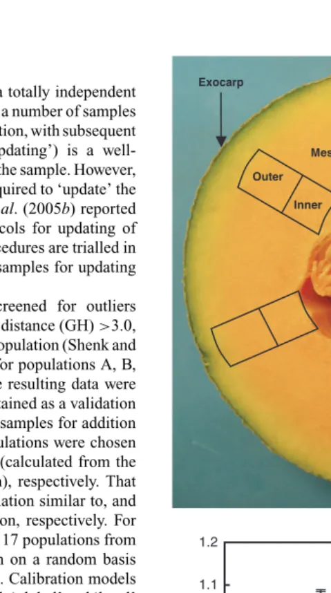
(4) 4. Australian Journal of Agricultural Research. J. A. Guthrie et al.. Model updating. Results and discussion Attribute distribution and light penetration In the inner mesocarp, TSS content was highest around the equator of the fruit and lessened towards both ends, but more so towards the proximal end. However, in the outer mesocarp there was little difference along the length of the fruit. Within the fruit, TSS content increased from the skin to the seed cavity and was highest around the vascular bundles near the seed cavity (Fig. 1a, b). There was no significant variation in TSS around the equator of the fruit, with reference to the part of the fruit in contact with the ground or with reference to the position of vasculature. The difference in TSS levels between various parts of an individual fruit’s flesh was as great as 6–7% TSS and averaged approximately 4% TSS overall. These observations reinforce the need to take both spectroscopic and reference values from the same area on the fruit. Ito et al. (1999) chose to base spectroscopic assessment of melons on the calyx end because ‘the flesh in the calyx end of melon fruit is thinner than that in other parts’. Certainly the chlorophyll-containing mesocarp layer is thinner in this region, and the mesocarp layer is thinner overall. However, the variation between the inner and outer mesocarp is similar to that in other regions of the fruit (Fig. 1b). As melon fruit is not perfectly spherical, but has a slightly proximal to distal elongation, fruit is mechanically orientated on conveyor systems to lie with the fruit long axis parallel to the direction of movement. Thus, 1 side of the fruit equator. Exocarp. (a). Mesocarp Outer Vascular tissue Inner. 1.2. (b) 1.1. % of maximum TSS value. The use of a model to predict attribute levels of a totally independent population is often compromised. The inclusion of a number of samples from the new population into the calibration population, with subsequent redevelopment of the MPLS model (‘model updating’) is a wellaccepted procedure to encompass new variation in the sample. However, there is no rule defining the number of samples required to ‘update’ the model. Guthrie and Walsh (2001) and Guthrie et al. (2005b) reported on the use of a range of sample selection protocols for updating of mandarin TSS models, and the recommended procedures are trialled in the current study. In those studies, the use of 20 samples for updating was recommended. Each validation population was initially screened for outliers (defined as samples with a weighted Mahalanobis distance (GH) >3.0, using the scores and loadings from the validation population (Shenk and Westerhaus 1991). These outliers were removed for populations A, B, and C (6, 5, and 7 outliers, respectively), and the resulting data were divided randomly into 2 sets. One set (2/3) was retained as a validation population and the other set used for selection of samples for addition to the calibration population. Two validation populations were chosen that exhibited a low and high average GH value (calculated from the scores and loadings of the calibration population), respectively. That is, these 2 populations will represent a new population similar to, and markedly different from, the calibration population, respectively. For addition to the calibration population (comprising 17 populations from years 1999 and 1998), new samples were chosen on a random basis from the subset of the validation population (1/3). Calibration models were then developed using MPLS regression in both ‘global’ and ‘local’ WINISI procedures.. 1.0 0.9 0.8 0.7 0.6 0.5 0. 1. 2. 3. 4. 5. 6. 7. 8. 9. 10. 11. 12. Fruit slices. Fig. 1. Spatial distribution of the attribute of total soluble solids (TSS) in rockmelon fruit (variety Doubloon): (a) image of fruit indicating location of sampling; (b) TSS distribution. Fruit was cut transversely into 12 slices. Each slice was assessed for % TSS in the inner (open symbols) and outer mesocarp (solid symbols), adjacent (triangle) and between (circle) vascular tissue (12 locations per slice). Data points represent the average of 30 values (6 positions per fruit, 5 fruits), normalised to the TSS concentration at slice 6 (equatorial) of the inner mesocarp. Slices are numbered from proximal to distal end of the fruit.. is presented uppermost, and as such represents a large target area for a NIR spectrometer suspended above a grading line. To facilitate in-line fruit grading, we chose to assess fruit in an equatorial position on the fruit. Light penetrated further through the centre of the fruit (i.e. through the seed cavity) than through the mesocarp layers (Fig. 2). Light penetrated through the bulk of the fruit, propagating through the mesocarp layers, but was strongly.
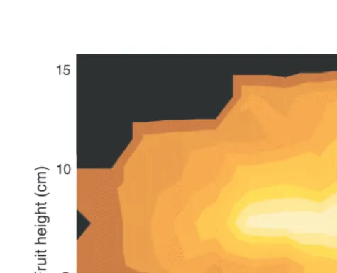
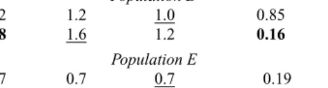
(5) NIR prediction of melon total soluble solids. Australian Journal of Agricultural Research. 1.5. 1050. 15. 1.4. Fruit height (cm). 10. A. 5. 27–30 24–27 21–24 18–21 15–18 12–15 9–12 6–9 3–6 0–3. Wavelength end (nm). 1000 33–36 30–33. 5. 1.3 950 1.2 900. 1.1 1.0. 850. 0.9 800 0.8 700. 0 0. 5. 10. 750. Fig. 2. Light penetration through a rockmelon fruit. Light (100-Watt tungsten-halogen lamp) illuminated position A on the equator of the fruit. Fruit was sliced longitudinally in a perpendicular plane to the lamp–fruit axis and light emergent from the cut surface recorded from 1-cm-diameter patches using the peak wavelength of approximately 820 nm. Data of a virtual longitudinal slice in the plane of the lamp–fruit axis (for a fruit position with stem end uppermost) are presented. Scale bar is in arbitrary units of detector analogue to digital counts.. absorbed by the exocarp layers. With a 100-Watt lamp, light was detectable in transmission through the fruit only once the skin (5 mm depth) was removed. We conclude that the skin of the intact fruit presents the greatest obstacle to the penetration of NIR radiation. This is more so than in other fruit (e.g. apples, stone fruit) because of the relative thickness and often irregular (e.g. netted) surface of rockmelon fruit. Spectral window and data treatment The spectral window used in PLS calibration model development for TSS was optimised in terms of RMSEC using the moving PLS interval algorithm described above. Low RMSEC values for TSS were obtained for a window beginning between 680 and 740 nm, and finishing between 900 and 955 nm, although acceptable results were obtained up to 1050 nm (Fig. 3). The minimum RMSEC for TSS (0.26%) was recorded for a start wavelength of 709 nm and a finish wavelength of 917 nm, surrounded by an area (or island) of low RMSEC values, suggesting a stable spectral region for TSS model development. Although the RMSEC was used to compare the relative spectral regions, the final ‘proof ’ of a model is in its validation statistics rather than the calibration statistics. Using a model developed with a combined population of years 1 (1998) and 2 (1999) (17 populations across varieties and growing districts) to predict the 5 populations from year 3 (2000), the best data pre-treatment routine was second-derivative. 850. 900. 950. Wavelength start (nm). 15. Fruit width (cm). 800. Fig. 3. Calibration model performance [root mean square standard error of calibration (RMSEC)] for varying spectral windows (start and end wavelengths varied). Partial least squares calibration models were based on the combined populations from year 1998 and 1999 (17 populations) for total soluble solids (mean = 8.9% TSS and s.d. = 1.73% TSS).. absorbance data without scatter correction (Table 2). The use of derivative spectra is a very effective method for removing both the baseline offset and the slope from a spectrum (Norris 1983). The full short-wave NIR region (695–1045 nm) was not significantly better than the restricted region (722–945 nm) in terms of RMSEP, but was significantly better (5% level) with regard to bias in 4 out of the 5 independent validation populations (Table 2). Both windows encompass the spectrally significant 910-nm third overtone of CH stretching, which will primarily be due to sucrose in melon fruit. Therefore, second-derivative absorbance data without scatter correction, over a 695–1045 nm wavelength range, were subsequently used in all calibration model development. Calibration model statistics varied across the 22 populations, with root mean squared error of crossvalidation (RMSECV) ranging from 0.63 to 1.2% TSS and the SDR from 1.1 to a high of 2.7 (Table 1). In prediction of independent datasets, the models gave similar or better results (in terms of RMSEP, see Tables 2 and 3) than those obtained by other researchers [e.g. Dull et al. (1990), RMSEP of 1.9% TSS; Guthrie et al. (1998), RMSEP of 0.9% TSS; Greensill and Walsh (2000), RMSEP of 0.7% TSS] but inferior to those obtained by Aoki et al. (1996), RMSEP of 0.4% TSS. However, Aoki et al. (1996) used a population with a lower s.d. (0.76% TSS) than any population in the current study. Regression method The settings for the ‘local’ procedure were optimised at 100 samples, 25 MPLS factors, and 1 MPLS factor removed..
(6) 6. Australian Journal of Agricultural Research. J. A. Guthrie et al.. Table 2. Optimisation of data pre-treatment in terms of derivative treatment (none, first, or second order) and 2 wavelength regions (695–1046, 722–945 nm) for TSS calibration Model performance is reported in terms of prediction of 5 independent populations of rockmelon fruit (year 3 harvest). The model was developed using the combination of 17 populations (year 1 and 2 harvests, n = 1467, mean = 8.9%, s.d. = 1.73%, and range of 4.8–15.2% TSS). For each population, the treatment with the lowest overall RMSEP was presented in bold (but not underlined). The corresponding bias was also bolded. These values were then compared with that related to the lowest RMSEP in the other wavelength window, and that related to the highest RMSEP value in the other derivative condition of the same wavelength region (value underlined). These values were tested for significance (95% probability level), with significantly different values shown in bold Variance (RMSEP) Absorb. 1st Deriv. 2nd Deriv.. Absorb.. bias 1st Deriv.. 2nd Deriv.. 695–1046 nm 722–945 nm. 1.0 1.1. 1.1 1.3. Population A 1.0 1.0. 0.24 −0.42. 0.22 0.86. 0.04 0.28. 695–1046 nm 722–945 nm. 0.7 0.8. 0.6 0.9. Population B 0.6 0.6. 0.18 −0.53. 0.05 0.69. −0.09 0.10. 695–1046 nm 722–945 nm. 1.1 1.1. 1.1 0.9. Population C 1.3 1.4. −0.58 −0.68. −0.69 −0.28. −0.87 −1.05. 695–1046 nm 722–945 nm. 1.2 0.8. 1.2 1.6. Population D 1.0 1.2. 0.85 0.16. 0.84 1.5. 0.70 0.92. 695–1046 nm 722–945 nm. 0.7 0.8. 0.7 1.1. Population E 0.7 0.7. 0.19 −0.40. 0.22 0.92. 0.08 0.37. As noted above, the apparent model ‘over-fitting’ inherent in the use of 25 MPLS factors is not an issue because of the use of the model for the prediction of the 1 sample only. However, a limitation of the WINISI ‘local’ procedure is that it forces the elimination of the first MPLS factor. This step may be logical for reflectance spectra in which the first factor can be associated with explanation of scattering properties of the sample. However, this step is not logical for partial transmission spectra as used in this study. Using the MPLS ‘global’ procedure the residuals (predicted – actual) for the prediction of population C were independent of analyte level, whereas those for population A increased with analyte levels (data not shown). It was therefore expected that the ‘local’ procedure might improve prediction in the case of population A. The prediction results of the same independent validation populations (Populations A and C from 2000) obtained from calibration models developed with the WINISI MPLS ‘global’ procedure were better than those obtained from the ‘local’ procedure (Table 3). The use of alternatives to ‘global’ MPLS, including ‘local’ neural networks and support vector machines, should be further explored. Model updating As expected, the prediction performance of a model on an independent population was determined by the average GH of that population (calculated using calibration model scores. Table 3. Prediction statistics (RMSEP and bias % TSS) for validation populations A and C from year 2000 predicted by the calibration from the combined population of years 1998 and 1999 (17 populations, n = 1467) using both ‘global’ and ‘local’ WINISI MPLS procedures MPLS calibration procedure Global Local. Population A s.d. = 1.80% TSS RMSEP bias 1.1 1.5. 0.04 0.24. Population C s.d. = 1.44% TSS RMSEP bias 1.3 2.1. −0.87 −1.60. and loadings) (Fig. 4). Better initial prediction occurred when the average GH value was low. Model updating, using a small number of samples from the validation population, offers an alternative to the development of an entirely new model. The effect of model updating to improvement in prediction performance of an independent validation population depended on the average GH value of the validation population. A greater improvement in both prediction RMSEP and bias values was demonstrated in both the WINISI procedures of ‘global’ and ‘local’ MPLS calibration models following sample addition (model updating) when the validation population exhibited a higher initial average GH value (Figs 4 and 5). A stabilisation of both the RMSEP and bias values occurred with the addition of approximately 15 samples (Fig. 4), for both ‘global’ and ‘local’ WINISI procedures (Fig. 5)..
(7) NIR prediction of melon total soluble solids. Australian Journal of Agricultural Research. 1.30. 7. 2.2. 1.25. RMSEP (%TSS). RMSEP (%TSS). 2.0 1.20. 1.15. 1.10. 1.8. 1.6. 1.05. 1.00. 1.0. 0.0. 0.5. –0.2. 0.0. bias (% TSS). bias (% TSS). 1.4. –0.4. –0.6. –1.0. –0.8. –1.5. –1.0. –2.0. 1.2. 2.5. 1.0. 2.0. Av. GH. Av. GH. –0.5. 0.8. 1.5 0.6 1.0 0.4 0. 5. 10. 15. 20. 25. 30. 0. 35. Fig. 4. Prediction statistics for ‘global’ WINISI modified partial least squares regression models in prediction of total soluble solids in rockmelon fruit for 2 independent (of calibration populations) validation populations. The average of global Mahalanobis distance (GH) of samples in the validation population was calculated using calibration model scores. The initial calibration population comprised the combined population of years 1998 and 1999 (17 populations). Populations from year 2000 [2 populations: A (closed squares) and C (open squares)] were used as validation populations, less the one-third randomly selected samples that were used for ‘model updating’ (addition to the calibration population). Samples for ‘model updating’ were chosen randomly from this population.. 5. 10. 15. 20. 25. 30. 35. Number of samples. Number of samples. Fig. 5. Prediction statistics for ‘local’ WINISI modified partial least squares regression models in prediction of total soluble solids in rockmelon fruit for 2 independent (of calibration populations) validation populations. The data populations used and treatments undertaken were the same as in Fig. 4.. population is ascribed to a greater leverage on the MPLS calibration. However, it is surprising that so few samples (i.e. n = 15) can influence a large calibration population (n = 1467). Conclusions. This result is consistent with the work reported for mandarins (Guthrie et al. 2005b). The greater effect of sample addition-model updating for a high GH validation. Model performance for prediction of TSS in intact rockmelon fruit was inferior to previous work on mandarins (Guthrie et al. 2005a, 2005b). This was ascribed to the.
(8) 8. Australian Journal of Agricultural Research. J. A. Guthrie et al.. heterogenous distribution of TSS (sugars) within the fruit and poor penetration of light through the irregular fruit skin. Data selection and pre-treatment were optimised in terms of prediction performance. The use of secondderivative absorbance data with scatter correction, using a spectral window of 695–1045 nm, is recommended. The WINISI MPLS calibration ‘global’ procedure was superior in terms of RMSEP and bias to the ‘local’ procedure in prediction of independent validation populations. Prediction statistics (RMSEP and bias) can be improved with the addition of approximately 15 samples from the validation population, as found for mandarins (Guthrie et al. 2005b). Acknowledgments Funding support was received from Horticulture Australia (Project No. VG97109). We acknowledge the supply of fruit and support from the growers of the Australian Melon Association. Aspects of this work have been published in Proceedings of the 8th International Conference on Near Infrared Spectroscopy, Essen, Germany (Ed. AMC Davies), 1998, under the title ‘Robustness of NIR calibrations for soluble solids in intact melon and pineapple’. Authors were JA Guthrie, BB Wedding and KB Walsh. References Aoki H, Kouno Y, Matumoto K, Mizuno T, Maeda H (1996) Non-destructive determination of sugar content in melon and watermelon using near infrared (NIR) transmittance. In ‘International Conference on Tropical Fruits’. Kuala Lumpur, Malaysia. (Eds S Vijaysegaran, M Pauziah, MS Mohamed, S Ahmad) p. 35. (Malaysian Agricultural Research and Development Institute: Kuala Lumpur) Birth SG, Dull GG, Leffler RG (1990) Non-destructive determination of the solids content of horticultural products. Optics in Agriculture 1379, 10–15. Dull GG, Birth GS, Leffler RG (1989) Exiting energy distribution in honeydew melon irradiated with a near infrared beam. Journal of Food Quality 12, 377–381. Dull GG, Leffler RG, Birth GG, Smittle DA (1990) Instrument for non-destructive measurement of soluble solids in honeydew melons. In ‘1990 International Winter Meeting’. Chicago, IL. pp. 735–737. (The American Society of Agricultural Engineers: Illinois) Fearn T (1996) Comparing standard deviations. NIR News 7, 5–6. Greensill CV, Walsh KB (2000) A remote acceptance probe and illumination configuration for spectral assessment of internal attributes of intact fruit. Measurement Science & Technology 11, 1674–1684. doi: 10.1088/0957-0233/11/12/304 Guthrie JA, Reid DJ, Liebenberg CJ, Walsh KB (2005a) Assessment of internal quality attributes of mandarin fruit. 1. NIR calibration model development. Australian Journal of Agricultural Research 56, 000–000. Guthrie JA, Reid DJ, Walsh KB (2005b) Assessment of internal quality attributes of mandarin fruit. 2. NIR calibration robustness. Australian Journal of Agricultural Research 56, 000–000.. Guthrie JA, Walsh KB (2001) Assessing and enhancing near infrared calibration robustness for soluble solids content in mandarin fruit. In ‘10th International Conference on Near Infrared Spectroscopy’. Kyonjgu, Korea. (Eds AMC Davies, RK Cho) pp. 151–154. (NIR Publication: Chichester, UK) Guthrie JA, Wedding B, Walsh K (1998) Robustness of NIR calibrations for soluble solids in intact melon and pineapple. Journal of Near Infrared Spectroscopy 6, 259–265. Ito H, Ippoushi K, Higashio H (1999) Non-destructive estimation of soluble solids in intact melons by non-contact mode with a fibre optic probe. In ‘9th International Conference Near Infrared Spectroscopy’. Verona, Italy. (Eds AMC Davies, R Giangiacomo) pp. 859–862. (NIR Publications: Chichester, UK) Kawano S (1994) Non-destructive NIR quality evaluation of fruits and vegetables in Japan. NIR News 5, 10–12. Lammertyn J, Peirs A, De Baerdemacker J, Nicolai B (2000) Light penetration properties of NIR radiation in fruit with respect to nondestructive quality assessment. Postharvest Biology and Technology 18, 121–132. doi: 10.1016/S0925-5214(99)00071-X Lester G, Shellie KC (1992) Postharvest sensory and physicochemical attributes of honey dew melon fruits. HortScience 27, 1012–1014. McGlone VA, Fraser DG, Jordan RB, Kunnemeyer R (2003) Internal quality assessment of mandarin fruit by vis/NIR spectroscopy. Journal of Near Infrared Spectroscopy 11, 323–332. McGlone VA, Kawano S (1998) Firmness, dry-matter and soluble-solids assessment of postharvest kiwifruit by NIR spectroscopy. Postharvest Biology and Technology 13, 131–141. doi: 10.1016/S0925-5214(98)00007-6 Mutton LL, Cullis BR, Blakeney AB (1981) The objective definition of eating quality in rockmelons (Cucumis melo). Journal of the Science of Food and Agriculture 32, 385–390. Norris KH (1983) Using gap derivatives as pre-processing for quantitative models – Food Research and Data Analysis. In ‘Proceedings of the 1982 IUFST Symposium’. Oslo, Norway. (Ed. H Martens) pp. 46–47. Peiris KHS, Dull GG, Leffler RG, Kays SJ (1998) Near-infrared spectroscopic method for non-destructive determination of soluble solids content of peaches. Journal of the American Society for Horticultural Science 123, 898–905. Shenk JS, Westerhaus MO (1991) Population definition, sample selection and calibration procedures for near infrared reflectance spectroscopy. Crop Science 31, 469–474. Shenk JS, Westerhaus MO (1997) Investigation of a LOCAL calibration procedure for near infrared instruments. Journal of Near Infrared Spectroscopy 5, 223–232. Sugiyama J (1999) Visualization of sugar content in the flesh of a melon by near-infrared imaging. Journal of Agricultural and Food Chemistry 47, 2715–2718. doi: 10.1021/jf981079i Tsuta M, Sugiyama J, Sagara Y (2002) Near-infrared imaging spectroscopy based on sugar absorption band for melons. Journal of Agricultural and Food Chemistry 50, 48–52. doi: 10.1021/jf010854i Walsh KB, Guthrie JA, Burney J (2000) Application of commercially available, low-cost, miniaturised NIR spectrometers to the assessment of the sugar content of intact fruit. Australian Journal of Plant Physiology 27, 1175–1186. Yamaguchi M, Hughes DL, Yabumoto K, Jennings WG (1977) Quality of cantaloupe muskmelons: variability and attributes. Scientia Horticulturae 6, 59–70. doi: 10.1016/0304-4238(77)90079-6. Manuscript received 5 April 2005, accepted 23 November 2005. http://www.publish.csiro.au/journals/ajar.
(9)
Figure
+2

Related documents