Assessing sampling designs for determining fertilizer practice from yield data

Patron: Her Majesty The Queen

Rothamsted Research

Harpenden, Herts, AL5 2JQ

Telephone: +44 (0)1582 763133

Web: http://www.rothamsted.ac.uk/

Rothamsted Research is a Company Limited by Guarantee Registered Office: as above. Registered in England No. 2393175. Registered Charity No. 802038. VAT No. 197 4201 51. Founded in 1843 by John Bennet Lawes.

Rothamsted Repository Download

A - Papers appearing in refereed journals

Muhammed, S. E., Marchant, B. P., Webster, R., Whitmore, A. P., Dailey,

A. G. and Milne, A. E. 2017. Assessing sampling designs for determining

fertilizer practice from yield data. Computers and Electronics in

Agriculture. 135 (1 April), pp. 163-174.

The publisher's version can be accessed at:

•

https://dx.doi.org/10.1016/j.compag.2017.02.002

The output can be accessed at:

https://repository.rothamsted.ac.uk/item/8v3xz/assessing-sampling-designs-for-determining-fertilizer-practice-from-yield-data

.

© 2017. CC-BY terms apply

Original papers

Assessing sampling designs for determining fertilizer practice from yield

data

S.E. Muhammed

a

, B.P. Marchant

b

, R. Webster

a

, A.P. Whitmore

a

, G. Dailey

a

, A.E. Milne

a,⇑

a_{Rothamsted Research, Harpenden, Hertfordshire AL5 2JQ, UK} b

British Geological Survey, Keyworth, Nottingham NG12 5GG, UK

a r t i c l e i n f o

Article history:

Received 18 December 2015

Received in revised form 2 February 2017 Accepted 5 February 2017

Available online 17 February 2017

Keywords: Yield maps Phosphorus Sampling Plant nutrients Variograms

a b s t r a c t

Many farmers sample their soil to measure the concentrations of plant nutrients, so as to decide how much fertilizer to apply. Now that fertilizer can be applied at variable rates farmers want to know whether maps of nutrient concentration made from grid samples or of field subdivisions (zones within their fields) are merited: do such maps lead to greater profit than would a single measurement on a bulked sample for each field when all costs are taken into account? We have examined the merits of grid-based and zone-based sampling strategies over single field-based averages using continuous spatial data on wheat yields at harvest in six fields in southern England and simulated concentrations of phos-phorus (P) in the soil. We have taken into account current prices of wheat, P fertilizer and sampling and laboratory analysis. Variograms of yield provide guides for sampling. We show that where variograms have large variances and long effective ranges grid-sampling and mapping are feasible and have large probabilities of being cost-effective. Where effective ranges are short, sampling must be dense to reveal the spatial variation and be expensive, and variable-rate application of fertilizer is likely to be impracti-cable and almost certainly not cost-effective. We found zone-based sampling was less likely to be cost effective in a similar situation when the management zones were poorly correlated to P concentrations. Crown CopyrightÓ2017 Published by Elsevier B.V. This is an open access article under the CC BY license (http://creativecommons.org/licenses/by/4.0/).

1. Introduction

We have known for more than 150 years that shortages of phos-phorus and potassium in the soil limit crop growth. Thousands of experiments have been done to estimate the responses of crops to additions of these nutrients and to calculate the needs for fertil-izers. Farmers now want to use these results to vary their applica-tions within fields. Perhaps surprisingly, there are few reports linking variation in the concentrations of these elements in the soil to yields within individual fields on commercial farms. There are examples, however, where positive correlations were found for cereals (Frogbrook et al., 2002) and pastures (McCormick et al., 2009; Serrano et al., 2011). Many farmers in the United Kingdom sample their soil every four years to measure the nutrients, in par-ticular phosphorus (P) and potassium (K), in the soil so as to decide how much fertilizer to apply to their crops. Sampling is often done at points on a ‘W’ shape across each field, and then individual sam-ples are bulked before analysis in the laboratory (PDA, 2011). Even though this sampling configuration does not follow the principles of design-based statistics, it has been widely adopted by farmers

as the results are generally no less accurate than those obtained from stratified random sampling (Marchant et al., 2012). By bulk-ing the sample, however, all information on the variation of the nutrients across the field is lost, and so any local deficiency or excess is obscured. If a farmer wants to map the variation in nutri-ents across a field, so that fertilizer could be adjusted spatially, for example, then he or she should ideally sample the soil on a grid (with perhaps some additional points at closer spacings) and mea-sure the nutrient content in each sample of soil separately (Mallarino and Wittry, 2004; Sawchik and Mallarino, 2007; Fu et al., 2013). Kriging, which makes best use of such data, could then be used to map the variation in nutrients (Kravchenko, 2003; Webster and Oliver, 2007). To krige, however, one needs an accu-rate estimate of the variogram or covariance function for the vari-able of interest, and for that at least 100 measurements are needed (Oliver and Webster, 2014). This creates a problem because mea-suring the concentration of P or K of each sample in the laboratory is costly.

Often the reason for the variation in yield across a field will be obvious to the farmer. For example, the farmer might know that a particular part of the field is prone to drought and that this is a major cause of the variation in yield. If the farmer suspects a local nutrient deficiency then it would make sense to divide the land

http://dx.doi.org/10.1016/j.compag.2017.02.002

0168-1699/Crown CopyrightÓ2017 Published by Elsevier B.V.

This is an open access article under the CC BY license (http://creativecommons.org/licenses/by/4.0/).

⇑ Corresponding author.

E-mail address:[email protected](A.E. Milne).

Contents lists available atScienceDirect

Computers and Electronics in Agriculture

into management zones and estimate the nutrient status for each zone separately.

So, which of these three sampling approaches, commonly used by farmers and advisors, should be adopted in any particular situ-ation to apply P and K fertilizer spatially? It is a question taxing agricultural advisers who want to advise farmers on best practice for within-field sampling for plant nutrients—see, for example, Oliver and Kerry (2013), Mylavarapu and Wonsok (2014) and Hawkins et al. (2016). The grid-based approach should result in the most accurate prediction of fertilizer requirement (Mallarino and Wittry, 2004; Sawchik and Mallarino, 2007). But the money saved by varying the application of the fertilizer locally within fields to match the requirement of the crop might be less than the cost of sampling and measurement (Fleming et al., 2000; Mallarino and Wittry, 2004). The balance of the two, and therefore the merit of the approach, depend on the magnitude and variation of the nutrient content of the soil (Sawchik and Mallarino, 2007). These two variables can be determined accurately only from mea-surements made on samples. The variation can, however, be assessed indirectly from crop yields. Many farmers are already monitoring yields as they harvest their crops, and variation in the data they record is in many instances a reflection of the varia-tion in the availability of the nutrients in the soil (Stafford et al., 1999; Diker et al., 2004; Flowers et al., 2005). If the variation in yield is small then it is unlikely that the nutrients vary substan-tially. We know that factors other than nutrient supply can cause large variations in yield. Nevertheless, nutrient supply does domi-nate yield variation in many cases, and for present purpose we pro-ceed on that assumption. In such circumstancesLark et al. (2003) proposed metrics based on the variogram of yield data (which cap-tures the magnitude of variation of the yield) to assess the scope for variable rate management. Their approach was to use the met-rics as factors in a decision tree designed to determine the poten-tial for variable rate management.

In this context we aimed (i) to compare the merits of measuring plant nutrients by three sampling schemes (whole fields, zones within fields and grids) and (ii) to assess the extent to which yield maps might be used to determine the most cost-effective sampling. Which of the above sampling approaches is suitable for a given sit-uation depends on a farmer’s profit margin over the cost of fertilizer and soil sampling. It is not possible to do such a comparison in the field because the test requires perfect knowledge of how the nutri-ents vary across the field, we therefore resorted to simulation. In the approach presented here we simulated the variation in nutri-ents across fields from geostatistical models of the nutrinutri-ents and used these to test the cost effectiveness of each sampling scheme. We modelled the associated yield variation for each realization and explored the use of the metrics of the yield variogram to decide which sampling strategy was likely to be most cost-effective.

2. Method

2.1. Data

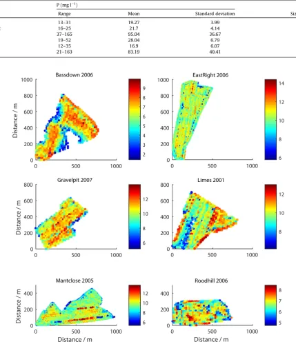
We collated yield data, denotedy, from monitors on board com-bine harvesters and measurements of extractable P, denotedz, in the soil for six fields on a farm near Newbury, England (Table 1). Soils were medium to heavy textured with slight to moderate stoniness. The yields were of winter wheat from the seasons 2001 to 2011 recorded at approximately 20-m intervals by the monitor. The measurements of Olsen extractable P (sodium bicar-bonate extract at pH 8.2) were made on a 100-m grid at 24–36 locations across each field.Fig. 1displays yield maps for the six fields for a single year.

2.2. Determining management zones

Several methods have been devised for creating management zones (Oliver and Webster, 1989; Fleming et al., 2000; Diker et al., 2004; Flowers et al., 2005; Zhang et al., 2009). The multivari-ate technique ofDray et al. (2006)has most recently been applied successfully by Peralta et al. (2015) for wheat farming and by Córdoba et al. (2016)for grain cropping more generally.

We created management zones from the yield data using a spa-tially smoothed version of a fuzzyk-means classification devised byLark (1998)(see alsoMilne et al., 2012). The data for the classi-fication consisted of yields of wheat forpyears at thennodes of a square grid at intervals of 10 m. We denote the grid coordinates as

xfx1;x2gand the yields in thepyears asy1ðxÞ;y2ðxÞ;. . .;ypðxÞ. From these data we created a classification by a ‘hard’k-means algorithm. We standardized each of they_j;j¼1_;2_{;. . .;}y_p to zero mean and variance of 1, denoted~yj. For this method we choosek, the number of classes. We divided the whole set of the standard-ized data into that number of classes in such a way as to minimize the trace or determinant of the within-classes variance–covariance matrix. Each grid node then belonged to one and only one of thek classes, and in general it resembled other members of its class more than the members of the other classes.

For fuzzy k-means classification we first define a measure of dissimilarity,d, between an individual nodeiand a classq. A con-venient measure is the Euclidean distance in the vector space:

diq¼

ffiffiffiffiffiffiffiffiffiffiffiffiffiffiffiffiffiffiffiffiffiffiffiffiffiffiffiffiffiffiffiffiffiffiffiffi Xp

j¼1 y~ij~yjq

2

r

; ð1Þ

where~yijis the standardized yield at nodeiin thejth year, andy~jqis the mean of~yin classqin that year.

Nomenclature

xfx1;x2g spatial coordinates in two dimensions y yield of crop

~

y standardized yield yr realized yield y0 target yield

z quantity of phosphorus, P z realization ofz

zfert quantity of fertilizer P zsoil initial quantity of P in the soil

ztotal zfertþzsoil

k the number of classes in thek-means classification

variogram parameters c0 nugget variance

c1 variance of spatially correlated structure a distance parameter

Costs

Gwheat price of grain, assumed to be £150 t1

Gfert price of P fertilizer, assumed to be £0.31 kg1

For this method we assume that each node belongs to some degree to every class, and we create a classification by minimizing a pooled ‘belongingness’, sayb:

b¼X k

q¼1

Xn

i¼1

d2iqu

x

iq; ð2Þ

in whichuiqis the degree of membership of nodeito classq, and

x

is the fuzzyness parameter.

The membership across all classes must sum to 1:

Xk

q¼1

uiq¼1: ð3Þ

The parameter

x

must lie between 1 (in which case we obtain a hard classification) and 2. We set

x

¼1:25 to create our classifications.

As above, we needed to choosek. We did this by experimenting with several values between 2 and 5 (the most that a farmer is likely to distinguish). For each class we then computed the normal-ized classification entropynðkÞ, proposed byDunn (1977):

nðkÞ ¼ 1

lnk Xk

q¼1

Xn

i¼1

1

nuiqlnuiq: ð4Þ

We then plotednðkÞagainstkand identified the value ofkat which

nðkÞfalls below the overall trend. This was the value we chose. The

0 500 1000

Distance / m

0 200 400 600

800 Gravelpit 2007

6 8 10 12

0 500 1000

0 200 400 600

800 Limes 2001

8 10 12

Distance / m

0 500 1000

Distance / m

0 200 400

Mantclose 2005

6 8 10 12

Distance / m

0 500 1000

0 200 400

Roodhill 2006

5 6 7 8

0 500 1000

Distance / m

0 200 400 600 800

1000 Bassdown 2006

2 3 4 5 6 7 8 9

0 500 1000

0 200 400 600 800

1000 EastRight 2006

6 8 10 12 14

Fig. 1.Maps of winter wheat yield from combine harvester yield monitors (t ha1

). Table 1

Soil type and summary statistics for measured P in the six study fields.

P (mg l1

)

Field name Range Mean Standard deviation Size of sample

Bassdown 13–31 19.27 3.99 28

Easton Right 16–25 21.7 4.14 24

Gravelpit 37–165 95.04 36.67 23

Limes 19–52 28.04 6.79 26

Mantclose 12–35 16.9 6.07 24

procedure is analogous to that in hard k-means classification in which the trace of the within-classes variance–covariance matrix or its determinant is plotted againstk.

The next step in the zonation is to smooth the classes. It turned out that the distributions of the memberships of the nodes were strongly bimodal, and so, followingLark (1998), we transformed them with the symmetric log-ratio to unimodal distributions. We smoothed the transformed membership (denoted u~iq) using a weighted average of the transformed memberships in circular neighbourhoods,R, of radiusr:

~ uiq¼

X

j2R

wði;jÞu~iq: ð5Þ

Like the original memberships, the transformed memberships must lie in the range 0–1 and must sum to 1. This means that the weights inRmust sum to 1.

The weights were derived from the variogram, Eq.(6). We can write a simple bounded model in general as

c

ðhÞ ¼c0þc1fðhÞ: ð6Þ

In this equationc0is a spatially uncorrelated variance, the ‘nugget

variance’, corresponding to white noise andc1is the spatially

corre-lated component of variance; their sum,c0þc1, constitute the ‘sill’.

The functionfðhÞdefines the form of the variogram and contains a distance parameter. The weights are obtained as

wði;jÞ ¼_X1fðhijÞ j2R 1fðhijÞ

for allj2R; ð7Þ

where hij is the separation in distance and direction, the lag, between nodesiandj. Note that only the functional form of the var-iogram and its distance parameter affect the weights; neitherc0nor

c1do so. The neighbourhoodRdefines the region over which the

membership values are smoothed, unless the variogram reaches its sill within it. In the latter case the effective range of the vari-ogram defines the smoothing region.

The farmer, of course, must have a hard classification; for prac-tical management he must have each position in the field belong-ing to one class and one class only. So the final stage in the zonation is therefore to assign each node to the class for which its smoothed membership is greatest.

Note that the size ofRaffects the results. The larger it is the greater is the smoothing. If R is small then the classification is likely to be too fragmented; if it is too large then the memberships will be smoothed too much and the final classes not sufficiently homogeneous.Lark (1998)proposed a coherency index to identify an appropriate radius forRdefined as

H¼Pk

g

a q¼1w

2 q

; ð8Þ

where

g

_ais the proportion of pairs of nodes within a distance

a

that belong to the same class, andwq is the proportion of nodes that belong to classq. The larger is the value ofH, the more spatially coherent are the classes. We chose

a

¼10pffiffiffi2 m (the distance between two points on the diagonal of our 10-m grid) so that we were effectively comparing each node with its neighbours along the rows, columns and diagonals on the grid.

2.3. Modelling phosphorus in soil

For each of the six fields, we used the measurements,z, of P to create realizations of P concentrations with plausible means and spatial variations that could differ from one management zone to another. Our data came from well managed fields, but we wanted our simulated values of P to limit the yield. Therefore we scaled the

measured data by 0.5 before fitting the models of spatial variation for all fields except Mantclose. We used a similar approach to that described byMarchant et al. (2012). First we standardized the measurements,zi;i¼1;2;. . .;n, to have a variance = 1 by dividing by the standard deviation, s, of the data to give values ~zi;i¼1;2;. . .;n. Then we characterized the mean and spatial vari-ation within each of thekzones of the field by fitting a linear mixed model to the transforms,~z:

~

z¼Mbþ

g

; ð9Þ

whereMis annkfixed effects design matrix which permits the mean concentrations to differ between zones. If theith value of~z

is in zonejthen the element inith row of thejth column ofMis 1, otherwise it is 0. The vectorbis of lengthkand contains the coef-ficients of the fixed effects (i.e. the mean concentration within each zone). The component

g

UNð0;VÞUwhere Nð0;VÞis a vector of spatially correlated random residuals with a normal distribution with zero mean and covariance matrixV, andUis a diagonal matrix where elementUði;iÞ ¼

r

jwhen theith datum ofzis in zonej(i.e. this is a zone-dependent scaling factor of the variance). If we assume second-order stationarity, so that the covariance function exists and can be obtained from the variogram parameters, then these and the fixed effects coefficientsbcan be estimated simulta-neously by residual maximum likelihood, REML, (Patterson and

Thompson, 1971). We assumed that the spatial variation is repre-sented by an isotropic exponential variogram model:

c

ðhÞ ¼ c0þc1 1exp

h a

; ð10Þ

in whichc0andc1are the nugget and spatially correlated

compo-nents of the variance, as mentioned above, and a is a distance parameter. The function approaches its maximum,c0þc1,

asymp-totically, and the distance 3ais often taken to be the effective range of the spatial correlation (seeWebster and Oliver, 2007). In the dis-cussion below we shall often refer to the ‘effective range’ with this meaning.

We simulated values for P on a 10 m10 m grid across each field using the Cholesky decomposition technique, also known as lower–upper or LU technique (Webster and Oliver, 2007). We used the variogram model that we fitted to the transformed data to cre-ate anttcovariance matrixCand scaled this for each zone inde-pendently asUCb Ub, wheretis the number of simulated points on the 10 m10 m grid andUb is a diagonal matrix where element b

Uði;iÞ ¼

r

jwhen theith simulated value is in zonej. This was then decomposed into its lower and upper triangular form where

b

UCUb¼LLT: ð11Þ

The simulated values,z_{, are then given by}

z ¼ sðLgþMsimbÞ; ð12Þ

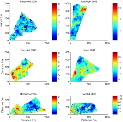
wheregis at1 vector of random numbers drawn from a standard normal distribution, andMsim is atk design matrix. If theith datum is in zonejthen the element in theith row of thejth column ofMsimis 1, otherwise it is 0.Fig. 2shows examples of the simulated values of P. For ease of calculating the yield response (see Sec-tion2.5) we converted our simulated P values to mg kg1_by

assum-ing the soil has a bulk density of 1.1 g cm3.

2.4. Modelling yield and quantifying its spatial variation

For each realization of simulated phosphorus,z_{, we simulated} the associated yields (y) using yield response models for P (see Sec-tion2.5) and computed experimental variograms from simulated yield values by the method of moments:

b

c

ðhÞ ¼ 1

2mðhÞ

X

mðhÞ

j¼1

yðxjÞ yðxjþhÞ

2

; ð13Þ

whereyðxjÞandyðxjþhÞare the simulated values at positionsxj andxjþhseparated by the lagh, which in the isoptropic case is the scalar distanceh, andmðhÞis the number of comparisons at that lag. By changinghwe obtained the ordered set to which we fitted exponential models, Eq. (10), by weighted least-squares approximation.

2.5. Yield response model

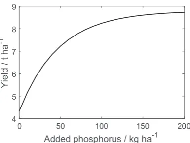
The yield response model for P was derived byMarchant et al. (2012)from published data (Syers et al., 2008; Johnston, 2005; Milford and Johnston, 2007; Johnston and Goulding, 1988). For every 1 kg of P added in fertilizer, we assumed that 0.18 kg is avail-able to the crop. We also assumed that this addition is contained in the top 30 cm of soil and the soil has a bulk density of 1.1 g cm3_.

This means that an addition of 1 kg P ha1leads to an increase in the concentration of this layer of

j

¼0:054 mg kg1_{. Thus the total}

nutrient available after addition of a quantity of fertilizerzfertwas

ztotal¼

j

zfertþzsoil; ð14Þ

wherezsoilis the initial concentration of the nutrient in the soil.

The yield response to added nutrients was modelled by

yr ¼ y0ð1AB

ztotalÞ; ð₁₅Þ

where yr is the realized yield,y0is target yields andA andBare

parameters. We set our target yield at 8.8 t ha1. The model param-eters wereA¼1:33 andB¼0:68 (seeFig. 3).

2.6. Sampling strategies

In each of the simulated fields, we compared three sampling schemes to see which would result in a treatment map that gave the greatest profit. The sampling schemes we considered were

(i) a W-shaped design across the whole field,

(ii) a zone-based scheme with W-shaped designs within each zone and

(iii) a grid-based scheme with samples taken on a 100 m100 m grid.

0 500 1000

Distance / m

0 200 400 600

800 Gravelpit 2007

20 30 40 50 60 70 80

0 500 1000

0 200 400 600

800 Limes 2001

5 10 15 20 25

Distance / m

0 500 1000

Distance / m

0 200 400

Mantclose 2005

10 20 30

Distance / m

0 500 1000

0 200 400

Roodhill 2006

20 40 60 80 100 120

0 500 1000

Distance / m

0 200 400 600 800

1000 Bassdown 2006

5 10 15 20 25 30

0 500 1000

0 200 400 600 800

1000 EastRight 2006

10 15 20

Fig. 2.Realizations of the simulated phosphorus concentrations (mg kg1

Each W-shaped design comprised 10 sampling points. In prac-tice soil samples taken according to schemes (i) and (ii) are bulked before analysis resulting in either a single value for each field or each zone within a field. To simulate these we calculated the aver-age of the nutrient values from the sample points on each W-shaped design. In grid-based designs the aim is to map the varia-tion in a nutrient so that fertilizer rates can be adjusted accord-ingly. Therefore these samples are not bulked before laboratory analysis; rather a measurement is made on each sample. The num-ber of sampling points depends on the size of the field, but typi-cally there are too few for prediction by kriging (the fields we considered here vary from 20 to 30 ha in size). The reason is that a minimum of about 100 points is needed for an accurate estimate of the variogram. Therefore inverse distance weighting is often used for the predictions instead of kriging, but these predictions are likely to be sub-optimal because practitioners do not know the spatial scale(s) of the variation.

2.7. Evaluation of sample designs

The profit from applying any of the strategies we have set out can be assessed simply as the difference between the cost of the measurements plus that of the fertilizer and price of the crop that is produced, in this case wheat. This is the net gain, which we denoteDfor unit area, thus:

D

¼yGwheatzfertGfertnGsample; ð16Þ

where Gwheat is the price of the grain, which we assumed to be

£150 t1_{; G}

fert is the price of fertilizer P, assumed to be

£0.31 kg1; nis the number of individual soil samples analyzed in the laboratory, each costingGsample¼£5, andyandzfertare the yield

and quantity of fertilizer added, respectively.

We estimated the nutrient concentration in the soil at each location on the 10 m10 m grid using each of the three sampling schemes. This resulted in a single estimate for the whole-field sam-pling scheme, an estimate for each zone for the zone-based scheme and a spatially varying estimate for the grid-based scheme. We denote these estimates ofzsoil bybzfield,bzzoneandbzgrid. Using these

estimates with Eqs.(14)–(16)we calculated the amount of fertil-izer that should be added (~zfert), noting that this value is not the

true optimum as it is based on the estimated nutrient supply not the true nutrient supply,zsoil.

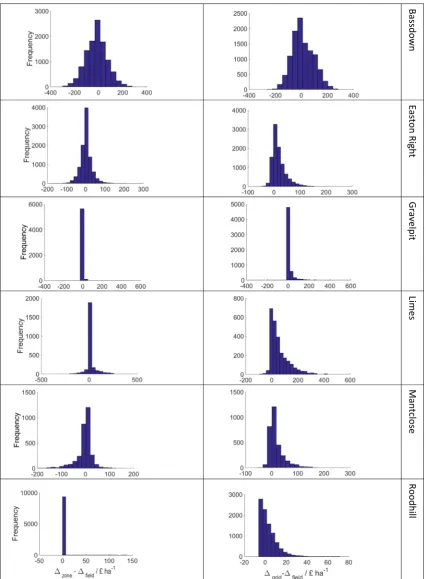
For each realization,i, of the fields we calculated the profit mar-gin under each sampling scheme. We computed the difference in profit margin given by the zone-based,DzoneðiÞ, and grid based,

DgridðiÞ, schemes compared with that of the field-based DfieldðiÞ

scheme. We also computed the excess fertilizer applied under the zone- and grid-based schemes and compared this with the field-based scheme.

2.8. Using metrics of variation to guide sampling strategies

For each set of simulations, we used multiple linear regression to see how much of the variation inDgridDfieldandDzoneDfield

could be explained by the distance parameter of the yield vari-ogram a and the variance parameter c1. More importantly we

wanted to compute the probability that the grid- or zone-based sampling strategies were more profitable than the field-based strategy for given parameters ofaandc1. For each field we fitted

the model

D

scheme

D

field ¼b0þb1aþb2c1þb3ac1; ð17Þ

to the data, where ‘scheme’ is ‘zone’ or ‘grid’. The assumption underlying the model is that the residuals are normally distributed about the mean prediction and that the standard error,sobsfor

pre-dicting a single observation is given by

s2

obs¼s2mseþb

T

VðbÞb ð18Þ

whereVðbÞis the covariance function for the parameter estimates

b fb0;b1;b2;b3gands2mseis the mean square error. From this we

calculated the probability thatDjDfield>0 for any given

combina-tion ofaandc1. We did a similar analysis for excess fertilizer.

3. Results

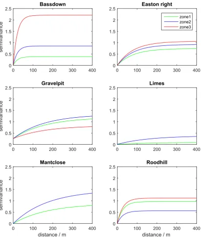
Based on the normalized classification entropy, two or three management zones were identified for each field (Table 2).Table 2 lists the parameters of the models fitted to the nutrient measure-ments, Eq.(9), and the fitted variograms are shown inFig. 4. The sill variances, c0þc1, vary from 0.09 to 2.23, and the effective

range from 63.0 m to 522.6 m showing substantial differences in the spatial structure of P between the fields.

Added phosphorus / kg ha

-1

0 50 100 150 200

Yield / t ha

-1

4 5 6 7 8 9

Fig. 3.Response of yield to added P to a soil with an Olsen extractable P of 2.5 mg kg1

.

Table 2

The number of management zones derived for each field and the parameters of the linear mixed model (Eq.(9)) fitted to the measured values of P. In each caser1¼1.

Field name

Number of zones

Fitted means St. dev. (s)

Mean times St. dev. Variogram structure parameters

bð1Þ bð2Þ bð3Þ sbð1Þ sbð2Þ sbð3Þ c0 c1 3aa Zone 2 scaling

parameterðr2Þ

Zone 3 scaling parameterðr3Þ

Bassdown 3 4.92 4.99 4.83 1.99 9.79 9.93 9.61 0.00 0.39 63.0 2.22 5.72

Easton Right

3 4.79 5.53 5.12 2.07 9.92 11.45 10.60 0.00 0.74 241.5 1.24 1.43

Gravelpit 3 2.27 2.78 1.92 18.33 41.61 50.96 35.19 0.26 0.93 471.9 1.15 0.61

Limes 2 3.81 4.21 – 3.40 12.95 14.31 – 0.01 0.08 480.0 4.46 –

Mantclose 2 2.81 2.92 – 6.07 17.06 17.72.31 – 0.00 0.88 522.6 1.68 –

Roodhill 3 2.06 1.40 2.70 20.21 41.63 28.29 54.57 0.00 0.97 84.9 0.58 1.16

a

3.1. Comparison of P estimated by the sampling schemes

The range of the simulated field averages for P (Table 3) were consistent with those reported by analytical laboratories for arable

fields in England and Wales (NRM Laboratories, 2017) and within the measured range (Table 1). For each realization we computed the difference in profit margin given by the zone-based (Dzone) and grid based (Dgrid) schemes compared with that of the

0

100

200

300

400

semivariance

0

0.5

1

1.5

2

2.5

Bassdown

0

100

200

300

400

0

0.5

1

1.5

2

2.5

Easton right

zone1 zone2 zone3

0

100

200

300

400

semivariance

0

0.5

1

1.5

2

2.5

Gravelpit

0

100

200

300

400

0

0.5

1

1.5

2

2.5

Limes

distance / m

0

100

200

300

400

semivariance

0

0.5

1

1.5

2

2.5

Mantclose

distance / m

0

100

200

300

400

0

0.5

1

1.5

2

2.5

Roodhill

Fig. 4.The spatial structure fitted to the phosphorus data in the six fields.

Table 3

Simulated field averages of soil P concentrations with the average difference in net profit for zone- and grid-based sampling compared with the field-based sampling across all simulations.

Field name Range of simulated averages of P (mg kg1

) Mean net profit (£ ha1

) Mean excess nutrient (kg ha1

)

Zone–Field Grid–Field Zone–Field Grid–Field

Profit SEa

Profit SE Profit SE Profit SE

Bassdown 19–21 13 0.81 12.1 0.75 2:49 0.17 1.07 0.17

Easton Right 17–25 0.93 0.23 14.8 0.21 0.14 0.11 1:9 0.10

Gravelpit 48–131 2.6 0.36 10.3 0.46 0.14 0.02 0.64 0.02

Limes 22–30 12.9 1.2 57.7 1.4 2:7 0.22 0:35 0.22

Mantclose 7–34 16.7 1.05 46.9 1.11 2:06 0.16 0:10 0.16

Roodhill 81–90 0:18 0.05 2.4 0.08 0.07 0.01 0.98 0.01

a

field-based (Dfield) scheme. Thus, the differences are (DgridDfield)

and (DzoneDfield) for the grid-based and zone-based values,

respectively. Table 3 reports the means and standard errors for these differences, which are also shown inFig. 5. In all cases the grid-based estimates gave larger profits than did the zone-based estimates. This was largely because the cluster classes were not significant factors in explaining the variation in the nutrients

(see supplementary information). The smallest differences between the zone-based estimate and the grid-based one were for the fields with the largest differences in mean concentrations of P between zones (Gravelpit and Roodhill). Bassdown had the smallest mean ofDzoneDfield, and this is likely to result from both

the small difference in mean values of P between the zones, sbð1Þ;sbð2Þ and sbð3Þ, and the short-range variation (effective

Bassdown

Easton Right

G

ravelp

it

Limes

Mantclose

Roodhi

ll

Zone-based sampling

Grid-based Sampling

Bassdown

Easton Ri

gh

t

Gravel

p

it

E

ff

e

ct

iv

e r

ange /

m

1 2 3 4

100 200 300 400 500 600

0.1 0.2 0.3 0.4 0.5 0.6 0.7 0.8 0.9

1 2 3 4

100 200 300 400 500 600

0.1 0.2 0.3 0.4 0.5 0.6 0.7 0.8 0.9

E

ff

e

ct

iv

e r

ange /

m

10 20 30 40

50 100 150 200 250 300

0.1 0.2 0.3 0.4 0.5 0.6 0.7 0.8 0.9

10 20 30 40

50 100 150 200 250 300

0.1 0.2 0.3 0.4 0.5 0.6 0.7 0.8 0.9

E

ff

e

ct

iv

e r

a

nge /

m

C₁

2 4 6 8 10 12

100 200 300 400 500 600 700 800 900

0.1 0.2 0.3 0.4 0.5 0.6 0.7 0.8 0.9

C₁

2 4 6 8 10 12

100 200 300 400 500 600 700 800 900

0.1 0.2 0.3 0.4 0.5 0.6 0.7 0.8 0.9

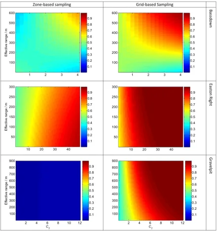
Fig. 6a.Maps of Bassdown, Easton Right and Gravelpit showing the probability that zone-based and grid-based sampling are more profitable than field-based sampling. Table 4

The percentage variance accounted for and model parameters for the multiple linear regression models (Eq.(17)) fitted to theDzoneDfieldandDgridDfielddata.

Field name Model parameters Percentage variance accounted for

b0 b1 b2 b3

Zone sampling

Bassdown 7:61 0:1907 7:82 0.1552 0.1

Easton Right 2:07 0:0082 4:275 0:00428 2.1

Gravelpita

7:2 0:018 12:53 0:0075 16:0

Limes 4:03 0:0008 3:882 0:00084 6:7

Mantclose 17:4 0:253 11:61 0:0378 3:8

Roodhilla

189.6 1:55 25:98 0:25 10:2

Grid sampling

Bassdown 6.01 0:013 10:03 0.2322 0.5

Easton Right 5.762 0.00653 6.629 0.01229 18.7

Gravelpit 8:065 0:00326 5.3 0.02439 50.2

Limes 9:03 0.1492 10.046 0:00218 33.9

Mantclose 4.654 0:0205 1:065 0.0049 45.0

Roodhill 7:117 0:0955 1.341 0.0145 21.9

range 63.0 m) which is smaller than the distance across feasible management zones. The largest mean profits were for Limes and Mantclose which have a long spatial structure (Fig. 4) with values of P in a treatable range (Table 3andFig. 3).

The distributions ofDzoneDfield are more symmetrically

dis-tributed than forDgridDfield for all fields except for Roodhill, (as

illustrated inFig. 5). The distributions ofDgridDfieldare positively

skewed. For Roodhill and Gravelpit a large number of realizations had values ofbzfield andbzzone that were not limiting (99% and 66%

respectively). This resulted in recommendations of no fertilizer application, and so DzoneDfield is simply the difference in

sam-pling costs. These correspond to the large peaks in the distributions

ofDgridDfield.

We also computed the difference in excess fertilizer applied when estimates were based on the zone-based (bzzone) and grid

based (bzgrid) sampling schemes compared with the field-based

(bzfield) scheme. We define excess fertilizer as the amount applied

over and above that which would have been applied if we had per-fect knowledge of the true variation in P across the field.Table 3 reports the means and standard error for these differences

(bzzonebzfieldandbzgridbzfield).

There was no consistent pattern to the mean responses. In some fields (Easton Right, Gravelpit and Roodhill) the field-based sam-pling resulted in less of an excess than the zone-based samsam-pling with positive differences and in some fields (Bassdown, Gravelpit and Roodhill) the field-based sampling resulted in less of an excess than the grid-based sampling (Table 3). Similarly there was no con-sistent pattern between grid- and zone-based sampling.

3.2. Assessing the extent to which yield maps can be used to predict the most appropriate sampling scheme

The parameters for the models fitted by multiple linear regres-sion are listed inTable 4along with percentage variance accounted

Zone-based sampling

Grid-based Sampling

Limes

Mantclose

Roodhill

E ffe c tiv e ra n g e

2 4 6 8 10 12

100 200 300 400 500 600 700 800 900 0.1 0.2 0.3 0.4 0.5 0.6 0.7 0.8 0.9

2 4 6 8 10 12

100 200 300 400 500 600 700 800 900 0.1 0.2 0.3 0.4 0.5 0.6 0.7 0.8 0.9 Ef fe ct iv e r ange / m

1 2 3 4 5 6

100 200 300 400 500 600 700 800 900 0.1 0.2 0.3 0.4 0.5 0.6 0.7 0.8 0.9

1 2 3 4 5 6

100 200 300 400 500 600 700 800 900 0.1 0.2 0.3 0.4 0.5 0.6 0.7 0.8 0.9 C₁ Ef fe ct iv e r ange / m

2 4 6 8 10

100 200 300 400 500 600 700 800 900 0.1 0.2 0.3 0.4 0.5 0.6 0.7 0.8 0.9 C₁

2 4 6 8 10

100 200 300 400 500 600 700 800 900 0.1 0.2 0.3 0.4 0.5 0.6 0.7 0.8 0.9

for. For Gravelpit, Mantclose and Roodhill the regression model was fitted to the subset of realizations wherebzfield orbzzone were

limiting. The models fitted toDzoneDfieldexplained very little of

the variation in the data. The variation inDgridDfield was better

explained, although the value for Bassdown were still small. The realizations for this site were generated from the model with a small effective range and the nugget to sill ratios of the realizations were in general larger than other sites (at least 37% larger, data not shown) indicating a relatively large component of unstructured variance.

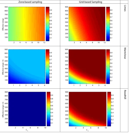
Figs. 6a and 6bshows the probability thatDzoneandDgridare

lar-ger thanDfield. In all cases the probability increases with bothc1

and the effective range (3a). This is also true ofDzoneDfield for

Gravelpit and Roodhill, but these sites are dominated by simula-tions wherebzfieldandbzzone where not limiting, and so the effects

are negligible.

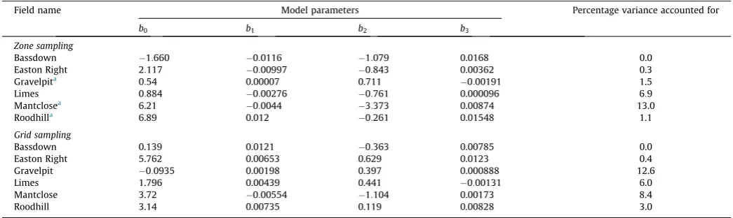
The multiple linear regressions showed that the effective range andc1explained very little of the variation in the excess fertilizer

data,bzzonebzfieldandbzgridbzfield(Table 5).

4. Discussion and conclusion

We have investigated, through simulation, the cost-effectiveness of three sampling strategies commonly used to guide fertilizer recommendations. We aimed to see if the variation cap-tured in yield monitor data could be used to determine which sam-pling strategy would be best in any given situation. The first option was the conventional single bulked sample for a whole field. The second was to delineate spatially coherent management zones from the yield data, sample the soil of each zone independently (zone-based sampling) and apply fertilizer (P in our case) in accord with the P content of the soil measured. The third option was to estimate the magnitude of the variation of P across the field, and judge from this how fertilizer might be applied at a variable rate. This required grid-based sampling.

Despite the expected increases in yield in response to additions of fertilizer, we know that there are situations in which there are inverse relations between nutrient concentration and yields (see, for example,Lake et al., 1997, for wheat andCox et al., 2003, for soya beans). It seems that in those situations the larger crops have extracted more of the nutrients and depleted the stock in the soil. We have shown that the advantages of using grid-and zone-based sampling strategies over field-zone-based ones vary from field to field. In our simulations, on average, the grid-based sampling performed better than the zone-based sampling. This was largely

because of the variation in the concentration of P, and the mean concentrations, did not differ sufficiently from one zone to another (even after scaling down the P measures used to model the varia-tion in soil P by 0.5). This is likely to be so for many arable fields in the UK because so much P has been added to them in the last 150 years. Other investigators (Mallarino and Wittry, 2004; Flowers et al., 2005; Sawchik and Mallarino, 2007) similarly found that grid-based sampling was better than the zone-based approach for estimating the likely responses of field crops to added fertilizer. Factors such as changes in water availability (due to variation in drainage or soil texture) or local infestations of weeds or disease will often be the main cause of large variations. In practice, many farmers would be able to explain the observed differences between proposed management zones and so be able to predict whether the zones were determined by differences in nutrient availability. This would provide valuable information on whether zone-based sam-pling was sensible.

The maps inFig. 6a and 6bshow that the probability of grid-based sampling’s being more profitable increases with both increases in effective range and in c1. Larger values ofc1 imply

large differences in nutrients, and a farmer might wish to apply fer-tilizer differentially in accord. This is feasible in practice only if the effective range is also large, and for two reasons. One is the diffi-culty of varying the application at a fine scale; the other is the cost of sampling and soil analysis on grids fine enough to map the con-centration of the nutrient in the soil.

Notice that the probability maps inFig. 6a and 6bchange from field to field. Note also that they are based on current prices of wheat and fertilizer and sampling costs, which are subject to vari-ation, and that our models might have introduced bias in prof-itability. Indeed, farmers will typically measure several soil variables at once (e.g. P, K, Mg and pH). Soil sampling may reveal anyone of these variables (or a combination of) to be the dominant cause of yield variation. Accurate quantification of the benefits of one sampling approach over another are therefore difficult, and so the absolute values shown in Figs. 6a and 6b should not be applied in other contexts, although, the principles hold. As varia-tion in yield at scales appropriate for management increases, so does the likelihood that grid-based sampling will be more prof-itable than a single field estimate.

Farmers and their advisors are building increasingly large data sets of crop yields, soil properties and previous management deci-sions. They should find these data valuable for managing their fields more effectively both to improve productivity and to reduce unnecessary inputs. The principles described here could be inte-grated into a decision-support system to help farmers decide when

Table 5

The percentage variance accounted for and model parameters for the multiple linear regression models (Eq.(17)) fitted to the^zzone^zfieldand^zgrid^zfield.

Field name Model parameters Percentage variance accounted for

b0 b1 b2 b3

Zone sampling

Bassdown 1:660 0:0116 1:079 0.0168 0.0

Easton Right 2:117 0:00997 0:843 0.00362 0.3

Gravelpita

0:54 0.00007 0.711 0:00191 1.5

Limes 0:884 0:00276 0:761 0.000096 6:9

Mantclosea _{6.21 0:0044 3:373 0.00874 13.0}

Roodhilla

6.89 0.012 0:261 0.01548 1.1

Grid sampling

Bassdown 0.139 0.0121 0:363 0.00785 0.0

Easton Right 5.762 0.00653 0.629 0.0123 0.4

Gravelpit 0:0935 0.00198 0.397 0.000888 12.6

Limes 1.796 0.00439 0.441 0:00131 6.0

Mantclose 3.72 0:00554 1:104 0.00173 8.4

Roodhill 3.14 0.00735 0.119 0.00828 3.0

variable-rate application of fertilizer might be cost effective and if so what sampling strategy to apply. This is the first step, then the farmer must decide how to vary the fertilizer spatially. The reliable prediction of how much fertilizer to apply depends not only on the quantification of the soil nutrient supply but also the yield poten-tial of the crop and the efficiency of nutrient uptake by the crop (Kindred et al., 2015). Predicting yield potential and the efficiency of nutrient uptake are substantial topics of research that can involve sensor technology, empirical analysis and simulation mod-elling (Dhital and Raun, 2016; van Wart et al., 2013; Kindred et al., 2015). In our study we followed the practices of agricultural advi-sors in the UK and considered zone-based and grid-based sampling schemes. The grid-based sampling scheme was on a 100-m grid, but in practice the variogram could be further used to optimize the grid sampling according to the cost of samples and the appar-ent dominant scale of spatial variation in the yield data.

Acknowledgement

This research was funded by the AHDB cereals and oilseeds pro-ject RD-2012-3785, using facilities funded by the Biotechnology and Biological Sciences Research Council (BBSRC). B. Marchant’s contribution is published with the permission of the executive director of the British Geological Survey (Natural Environment Research Council). We also thank Simon Griffin from SOYL for kindly providing us with the data.

Appendix A. Supplementary material

Supplementary data associated with this article can be found, in the online version, athttp://dx.doi.org/10.1016/j.compag.2017.02. 002.

References

Córdoba, M.A., Bruno, C.I., Costa, J.L., Peralta, N.R., Balzarini, M.G., 2016. Protocol for multivariate homogeneous zone delineation in precision agriculture. Biosyst. Eng. 143, 95–107.

Cox, M.S., Gerard, P.D., Wardlaw, M.C., Abshire, M.J., 2003. Variability of selected soil properties and their relationships with soybean yield. Soil Sci. Soc. Am. J. 67, 1296–1302.

Dhital, S., Raun, W.R., 2016. Variability in optimum nitrogen rates for maize. Agron. J. 108, 2165–2173.

Diker, K., Heermann, D.F., Brohdahl, M.K., 2004. Frequency analysis of yield for delineating zones. Precision Agric. 5, 435–444.

Dray, S., Legendre, P., Peres-Neto, P.R., 2006. Spatial modelling: a comprehensive framework for principal coordinate analysis of neighbouring matrices (PCNM). Ecol. Model. 196, 483–493.

Dunn, J.C., 1977. Indices of fuzziness and the detection of clusters in large data sets. In: Gupta, M.M. (Ed.), Fuzzy Automata and Decision Processes. North-Holland, New York, pp. 271–283.

Fleming, K.L., Westfall, D.G., Bausch, W.C., 2000. Evaluating management zone technology and grid soil sampling for variable rate nitrogen application. In: Robert, P.C., Rust, R.H., Larson, W.E. (Eds.), Proceedings of the 5th International conference on precision agriculture and other source management. ASA, CSSA, SSSA, Madison, WI, USA.

Flowers, M., Weisz, R., White, J.G., 2005. Yield-based management zones and grid sampling strategies. Agron. J. 97, 968–982.

Frogbrook, Z.L., Oliver, M.A., Salahi, M., Ellis, R.H., 2002. Exploring the spatial relations between cereal yield and soil chemical properties and the implications for sampling. Soil Use Manage. 18, 1–9.

Fu, W., Zhao, K., Jiang, P., Ye, Z., Tunney, H., Zhang, C., 2013. Field-scale variability of soil test phosphorus and other nutrients in grasslands under long-term agricultural managements. Soil Res. 51, 503–512.

Hawkins, E., LeBarge, G., Watters, H.D., Fulton, J., Culman, S., 2016. Developing a strategy for precision sampling. Ohio State University Extension. <http:// agcrops.osu.edu/newsletter/corn-newsletter/2016-37/developing-strategy-precision-soil-sampling>.

Johnston, A.E., 2005. Phosphorus nutrition in arable crops. In: Sims, J.T., Sharpley, A. N. (Eds.) Phosphorus: Agriculture and the environment. Agronomy Monograph No 46. ASA-CSSA-SSSA, Madison, WI, USA, pp. 495–519.

Johnston, A.E., Goulding, K.W.T., 1988. Rational potassium manuring for arable cropping systems. J. Sci. Food Agric. 46, 1–11.

Kindred, D., Milne, A.E., Webster, R., Marchant, B., Sylvester-Bradley, R., 2015. Exploring the spatial variation in the fertilizer-nitrogen requirement of wheat within fields. J. Agric. Sci. 153, 2421.

Kravchenko, A.N., 2003. Influence of spatial structure on accuracy of interpolation methods. Soil Sci. Soc. Am. J. 67, 1564–1571.

Lake, J.V., Bock, G.R., Goode, J.A. (Eds.), 1997. Precision Agriculture: Spatial and Temporal Variability of Environmental Quality. John Wiley & Sons, Chichester. Lark, R.M., 1998. Forming spatially coherent regions by classification of multivariate data: an example from analysis of maps of crop yield. Int. J. Geogr. Inf. Sci. 129, 83–98.

Lark, R.M., Wheeler, H.C., Bradley, R.I., Mayr, T.R., Dampney, P.M.R., 2003. Developing a Cost-Effective Procedure for Investigating Within-Field Variation of Soil Conditions. Project Report No 296. HGCA, London.

Mallarino, A.P., Wittry, D.J., 2004. Efficacy of grid and zone soil sampling approaches for site-specific assessment of phosphorus, potassium, pH, and organic matter. Precis. Agric. 5, 131–144.

Marchant, B.P., Dailey, A.G., Lark, R.M., 2012. Cost-Effective Sampling Strategies for Soil Management. Project Report No 485. Home-Grown Cereals Authority. At <http://cereals.ahdb.org.uk/media/252469/pr485.pdf>(last accessed November 2015).

McCormick, S., Jordan, C., Bailey, J.S., 2009. Within and between-field spatial variation in soil phosphorus in permanent grassland. Precis. Agric. 10, 262–276. Milford, G.F.J., Johnston, A.E., 2007. Potassium and nitrogen interactions. In:

Proceedings No 615. International Fertiliser Society, Leek, UK, pp. 1–22. Milne, A.E., Webster, R., Ginsburg, D., Kindred, D., 2012. Spatial multivariate

classification of an arable field into compact management zones based on past crop yields. Comput. Electron. Agric. 80, 17–30.

Mylavarapu, R.S., Wonsok, D.L., 2014. Nutrient Management Series, Soil Sampling Strategies for Precision Agriculture. University of Florida, Institute of Food and Agricultural Sciences.<http://edis.ifas.ufl.edu/pdffiles/SS/SS40200.pdf>. NRM Laboratories (2017). Soil Nutrient Status, Soil Summary 2015-2016. NRM

Laboratories, Bracknell, UK. <http://www.nrm.uk.com/files/documents/NRM-Soil-Summary-2015-2016-Opt03b.pdf>(last accessed Feb 2017).

Oliver, M.A., Kerry, R., 2013. Sampling and Geostatistics for Precision Agriculture. International Fertiliser Society, Colchester, UK.

Oliver, M.A., Webster, R., 1989. A geostatistical basis for spatial weighting in multivariate classification. Math. Geol. 21, 15–35.

Oliver, M.A., Webster, R., 2014. A tutorial guide to geostatistics: computing and modelling variograms and kriging. Catena 113, 56–69.

Patterson, H.D., Thompson, R., 1971. Recovery of inter-block information when block sizes are unequal. Biometrika 58, 545–554.

PDA, 2011. Soil Analysis: Key to Nutrient Management Planning, Leaflet 24. The Potash Development Association, York, UK.

Peralta, N.R., Costa, J.L., Balzarini, M., Franco, M.C., Córdoba, M., Bullock, D., 2015. Delineation of management zones to improve management of wheat. Comput. Electron. Agric. 110, 103–113.

Sawchik, J., Mallarino, A.P., 2007. Evaluation of zone soil sampling approaches for phosphorus and potassium based on corn and soybean response to fertilization. Agron. J. 99, 1564–1578.

Serrano, J.M., Pea, J.O., Marques da Silva, J.R., Shahidian, S., 2011. Spatial and temporal stability of soil phosphate concentration and pasture dry matter yield. Precis. Agric. 12, 214–232.

Stafford, J.V., Lark, R.M., Bolam, H.C., 1999. Using yield maps to regionalize fields into potential management units. In: Robert, P.C., Rust, R.H., Larson, W.E. (Eds.), Proceedings of the 5th International Conference on Precision Agriculture and Other Source Management. ASA, CSSA, SSSA, Madison, WI, USA, pp. 225–237. Syers, J.K., Johnston, A.E., Curtin, D., 2008. Efficiency of Soil and Fertilizer

Phosphorus Use: Reconciling Changing Concepts of Soil Phosphorus Behaviour with Agronomic Information. Bulletin 18. FAO, Rome. <ftp://ftp.fao. org/docrep/fao/010/a1595e/a1595e00.pdf> (last accessed November 2015). van Wart, J., Kersebaum, K.C., Peng, S., Milner, M., Cassman, K.G., 2013. Estimating

crop yield potential at regional to national scales. Field Crops Res. 143, 34–43. Webster, R., Oliver, M.A., 2007. Geostatistics for Environmental Scientists. John

Wiley & Sons, Chichester.