1
Topological Quantum Interplay between Magnetic Flux and Mass in an
Electron
Vincenzo Vinciguerra*
STMicroelectronics, Stradale Primosole 50, 95121, Catania, Italy.
*corresponding author email: vincenzo.vinciguerra@st.com
Abstract
A topological quantum interplay between the magnetic flux Φ and the mass has been investigated, for the case of an electron, by evaluating a gauge-invariant phase factor (a Wilson loop) linked to the electromagnetic gauge field
𝐴𝜇 of the particle. In particular, from this phase factor and the quantization of the magnetic flux variations, a
relationship between the mass at rest of the electron 𝑚𝑒 and its self-energy 𝛿𝑚, arising from radiative corrections,
has been obtained also within a QED approach. Besides, a formulation of an energy scale comparable to the energy at rest of an electron-positron pair is proposed. Remarkably, a reckoning of the Bohr’s energy of a 𝑊+𝑊− pair is compatible with constants and parameters usually employed within the electroweak theory and comparable to the energy at rest of an 𝑒−𝑒+ pair.
Keywords: electron, topology, magnetic flux quantization, charge, mass, electroweak theory, Bohr’s energy, W
boson vector.
PACS numbers: Relativistic electron and positron, 41.75.Ht, Topology, 02.40.Pc, Electroweak interactions, 12.15.-y, Atomic spectra, 32.30.-r, W bosons, 14.70.Fm.
1. Introduction
Of all the massive elementary particles [1] investigated in the standard model (SM) [2], electrons have been definitely central in the development of the semiconductor industry [3], being their properties, either classical or quantal, widely exploited in the whole set of integrated circuits made of downscaled solid state devices.
For technologists and experts involved in the investigation of matter, electrons are fundamental particles upon which devising explanations regarding atoms, molecules, condensed matter and general observed phenomena. Indeed, thanks also to the rise and reliability of computational methods, tested over the years and established on fundamental principles, scientists can implement today a set of theoretical frameworks to further understand the structure of matter. Examples are the ab-initio methods such as tight binding, Hartree Fock (HF) and self-consistent HF [4, 5]), as well as first principles methods, built on the theory of density functional (DFT) [6-9]. Their use has definitely had an impact on our understanding of quantum effects in solid state thin films (e.g. in the quantum integer and fractional Hall effect) [10] and in the development of new device technologies [11], too.
To complete the picture, the physical foundations of the methods illustrated above rely upon the theory of quantum electrodynamics (QED) [12-13] and its later developments within the
2
electroweak theory; making QED the most successful theory in predicting and describing the interaction of electrons with light in every aspect.
However, after more than a century from the discovery [14] of the electron as a fundamental building block of matter, the electron is still perceived mostly as an enigmatic particle in its essence. Indeed, the words of the scholar Wilczeck [15] confirms such a picture: "An electron is a particle and a wave; it is ideally simple, and unimaginably complex; it is precisely understood, and utterly mysterious; it is rigid, and subject to creative disassembly. No single answer does justice to reality”.
Recently topology [16] is receiving considerable attention by condensed matter’s physicists focusing on the properties of topological phases [17-18]. Nonetheless, topological arguments have been already introduced in physics in the past [19-23]. Indeed, the charge quantization conditions determined by the existence of magnetic monopoles [24, 25], the Arhanov-Bohm effect [26] and the Berry’s phase [27] are just acknowledged examples of topological properties arising in specific physical systems.
In general, topology gives us insights on how different parts of a structure are linked together, or can be connected by paths. The Königsberg’s bridge problem of Euler [28], the network of covalent bonds of atoms in a molecule [29], the structure of a LAN or a WAN [30] are also examples of topological structures that can occur in space configurations. More specifically, in geometry, surface topology investigates how paths (open or in loops) can be deformed equivalently and continuously without tears or cuts of the surface or, in a similar manner, how surfaces can be modified smoothly into one another (e.g. a cup into a donut!).
Topological aspects determining the quantization properties of the intrinsic magnetic flux of electrons and the significance of the magnetic flux quantization is acknowledged in the field of condensed matter [31-33] as determinant to understand the physics of superconducting state and proved experimentally by Deaver and Fairbank [34], as well as by Doll and Näbauer [35]. Later the role played by the quantization of magnetic flux was extended to the Quantum Hall effect [36, 37].
In this work, we investigate the role that a quantization of the intrinsic magnetic flux in a particle plays in determining its properties. In particular, we discuss the topological interplay occurring between the intrinsic magnetic flux of a charged lepton, namely an electron, and its mass.
3
More recently, Saglam [44] and Stein [45] proved that the magnetic flux of an electron in a hydrogen atom is also quantized and that the electron spin contributes to the quantized flux according to −2𝜋𝑐 〈𝑠̂〉/𝑒, where 〈𝑠̂〉 is the expectation value of the spin of the particle, −𝑒 is its electric charge and 𝑐 the speed of light. At the best of the knowledge of the author, no further extensive investigations have been reported so far on the topic.
The paper is organized as follows. First, the topological quantum interplay between the magnetic flux Φ and the mass, for the case of an electron, is investigated by evaluating a gauge-invariant phase factor associated with the Wilson loop of the electromagnetic field 𝐴𝜇 generated by the particle. In particular, from the phase factor and the quantization of the magnetic flux variations, a relationship between the mass at rest of the electron 𝑚0 and its self-energy 𝛿𝑚 is obtained also
within a QED approach. Hence, the formulation of an energy scale comparable with the energy at rest of an electron and compatible with constants and parameters usually employed within the electroweak theory is discussed. Finally the conclusions are reported.
2. Topological interplay between magnetic flux and mass
Whenever a particle of charge 𝑞 undergoes a space-time loop 𝐶, in the gauge field 𝐴𝜇generated by an electron, it is possible to evaluate a gauge-invariant quantity [46]
𝑒ℏ𝑐𝑖𝑞∮ A𝐶 𝜇𝑑𝑥𝜇|𝜓⟩ = 𝑒𝑖𝑞𝛼|𝜓⟩ (1)
that determines a phase shift 𝑞𝛼 of the state |𝜓⟩. From the derivative of eq. 1 with respect to 𝑞,
it results that the quantity ℏ𝑐𝑞 〈∮ A𝐶 𝜇𝑑𝑥𝜇〉 determines the phase 𝑞𝛼:
𝑞
ℏ𝑐〈∮ A𝐶 𝜇𝑑𝑥𝜇〉 = 𝑞𝛼. (2)
On the other hand, the gauge-invariant quantity on the first member of eq. 2 can be evaluated independently. For example, for the case of an electron at rest with spin up, in a semi-classical approach, it reads as:
〈∮ A𝐶 𝜇𝑑𝑥𝜇〉 = 𝑐−𝑒〈𝜑(𝑟⃗,𝑡)〉−𝑒 𝑇 − Φ(↑) =−𝑒2𝑐𝛿𝑚𝑒𝑠𝑐2𝑇 − Φ(↑) (3)
Where 〈𝜑(𝑟⃗, 𝑡)〉 is the expectation value of the time-component of the 4-vector potential 𝐴𝜇,
𝛿𝑚𝑒𝑠𝑐2 works as an electrostatic energy and the period 𝑇 is a characteristic time of the electron, which hereafter will be considered equal to 𝑇 =𝑚𝜋ℏ
𝑒𝑐2.
In order to calculate the magnetic flux of an electron we proceed by considering the line integral of the operator 𝐴⃗ on a closed circular loop 𝐶𝑟 = {𝑟(𝑡)|𝑡 = 0 → 𝑇} in the space-coordinates and average it over all possible values:
Φ = 〈∮𝐶 𝐴⃗⃗⃗∙ 𝑑𝑟⃗
𝑟 〉 = ∫ 𝑑𝑉 ∮ 𝜓
†(𝑟, 𝑡)𝐴⃗𝜓(𝑟, 𝑡)∙ 𝑑𝑟⃗ =
𝐶𝑟 ∫ 𝑑𝑉′ ∮ 𝜓
†(𝑟′, 𝑡′)𝐴⃗𝜓(𝑟′, 𝑡′)∙ 𝑑𝑟′⃗⃗⃗
4
In doing such a calculation, we can renominate 𝑟 in 𝑟′, as we expect that the variables 𝑟 and
𝑟′play a symmetric role.
In the semi-classical approach that we are following, according to eq. 4 the magnetic flux of an electron reads as:
Φ = 〈∮𝐶 𝐴⃗⃗⃗∙ 𝑑𝑟⃗
𝑟 〉 =
1
𝑐〈∫ ∮
𝑗⃗∙𝑑𝑟⃗ |𝑟⃗−𝑟⃗⃗⃗|′
𝐶𝑟 𝑑𝑉
′〉. (5)
In particular, for the case of an electron at rest, the magnetic moment 𝑚𝑧of an electron depends only on the spin, and it’s an observable that commutes with the Dirac’s Hamiltonian. It can be shown that:
Φ =1𝑐〈∫ ∮ 𝑗⃗∙𝑑𝑟⃗
|𝑟⃗−𝑟⃗⃗⃗|′
𝐶𝑟 𝑑𝑉
′〉 =4𝜋
𝑐 〈∫
1 2
(𝑟⃗×𝑗⃗)𝑧
|𝑟⃗−𝑟⃗⃗⃗|′ 𝑑𝑉
′〉 =4𝜋
𝑐 〈∫
𝑚𝑧𝜓†(𝑟′,𝑡′)𝜓(𝑟′,𝑡′)
|𝑟⃗−𝑟⃗⃗⃗|′ 𝑑𝑉
′〉
(6)
By reasoning on the quantized value that the magnetic moment 𝑚𝑧of an electron at rest assumes
for a state with spin up, we can deduce that:
Φ(↑)= − 4𝜋ℏ𝑐
2𝑒𝑚𝑒𝑐2〈∫
𝑒2𝜓†(𝑟′,𝑡′)𝜓(𝑟′,𝑡′)
|𝑟⃗−𝑟⃗⃗⃗|′ 𝑑𝑉
′〉. (7)
Hence the gauge-invariant quantity in eq. 2, can be evaluated as
〈∮ A𝐶 𝜇𝑑𝑥𝜇〉 =𝛿𝑚𝑚𝑒𝑠
𝑒
2𝜋ℏ𝑐
𝑒 . (8)
In the event, the phase in eq. 2 amounts to:
𝑞
ℏ𝑐〈∮ A𝐶 𝜇𝑑𝑥𝜇〉 = 𝑞 ℏ𝑐
𝛿𝑚𝑒𝑠
𝑚𝑒
2𝜋ℏ𝑐
𝑒 =
𝛿𝑚𝑒𝑠
𝑚𝑒
2𝜋𝑞
𝑒 . (9)
Moreover, in the hypothesis that there’s a certain arbitrariness in the choice of the charge 𝑞, we can choose it such that the gauge-invariant quantity in eq. 3 reads as:
𝑞
ℏ𝑐〈∮ A𝐶 𝜇𝑑𝑥𝜇〉 = 2𝜋𝑛, with 𝑛 𝜖 ℤ (10)
If this holds, the ratio between 𝛿𝑚𝑒𝑠 and 𝑚𝑒, must satisfy the equation:
𝛿𝑚𝑒𝑠
𝑚𝑒 =
𝑛
𝑞/𝑒. (11)
5 Φ(↑) = −4𝜋ℏ𝑐
𝑒 𝛿𝑚𝑒𝑠
𝑚𝑒 = −
4𝜋ℏ𝑐 𝑒
𝑛
𝑞/𝑒, (12)
for the case of an electron at rest with spin up, whereas, for an electron at rest with spin down the magnetic flux reads
Φ(↓) =4𝜋ℏ𝑐
𝑒 𝛿𝑚𝑒𝑠
𝑚𝑒 =
4𝜋ℏ𝑐 𝑒
𝑛
𝑞/𝑒. (13)
By imposing that the variation of the magnetic flux from spin down to spin up is equal to the quantum of the magnetic flux:
Φ(↓) − Φ(↑) =8𝜋ℏ𝑐
𝑒 𝑛
𝑞 𝑒
= 2𝜋ℏ𝑐
𝑒 , (14)
we obtain that the charge 𝑞 must satisfy the condition 𝑞 = 4𝑛𝑒.
Moreover, by defining 𝛿𝑚𝑒𝑚𝑐2= 4𝛿𝑚𝑒𝑠𝑐2 as an electromagnetic energy linked to the electron,
the magnetic flux can be expressed as:
Φ(↑) = −𝜋ℏ𝑐
𝑒
𝛿𝑚𝑒𝑚
𝑚𝑒 . (15)
From classical arguments it’s reasonable to expect such a dependence. In fact, the magnetic flux
Φ(↑) can be expressed in terms of the magnetic moment of the electron −𝜇𝐵, where 𝜇𝐵is the Bohr magneton, as:
Φ(↑) = −122𝜋ℏ𝑐𝑒 𝛿𝑚𝑒𝑚
𝑚𝑒 = −
𝑒 𝑚𝑒𝑐
ℏ 2
2𝜋𝛿𝑚𝑒𝑚𝑐2
𝑒2 = −𝜇𝐵
2𝜋𝛿𝑚𝑒𝑚𝑐2
𝑒2 . (16)
Indeed, the magnetic dipole moment 𝜇 determined by a current 𝑖 flowing, e.g. in a circular coil of radius 𝑟, is𝜇 = 𝑖𝜋𝑟2. The magnetic field generated at the center of the coil is 𝐵 =2𝜋𝑖𝑟 , and the
magnetic flux is approximately Φ = 𝐵𝜋𝑟2. By combining previous equations, we can express the magnetic flux in terms of the magnetic moment 𝜇. In fact, Φ = 𝐵𝜋𝑟2=2𝜋𝑖𝑟 𝜋𝑟2= 𝜇2𝜋𝑟. A
comparison with equation (16) provides the value 1𝑟=𝛿𝑚𝑒𝑒𝑚2𝑐2 .
By considering also possible QED corrections for the magnetic moment and indicating with
𝛿𝑚𝑒𝑠𝑐2 the contribution of the electrostatic energy, eq. 7 reads as:
Φ(↑)= −𝑔𝑠
2 8𝜋ℏ𝑐
2𝑒𝑚𝑒𝑐2𝛿𝑚𝑒𝑠𝑐
2 , (17)
where 𝑔𝑠 is the spin g-factor of the electron.
In conclusion, the gauge-invariant quantity appearing in eq. (2), can be expressed as:
𝑒
ℏ𝑐〈∮ A𝜇𝑑𝑥
𝜇
𝐶 〉 = 2𝜋
𝑔𝑠 2
𝛿𝑚𝑒𝑚
6
and being quantized in units of 2𝜋, it implies that there must exist an interplay between the magnetic flux and the mass, such that:
𝑔𝑠
2 𝛿𝑚𝑒𝑚
𝑚𝑒 = 1. (19)
Clearly such a conclusion has been achieved by pursuing a semi-classical approach. In fact, within the QED formulation it is not possible to evaluate a quantity such as the electrostatic self-energy of the electron. However, from the gauge-invariant quantity appearing in eq. (2), we can consider that 𝑑𝑥𝜇 = 𝛾𝜇𝑐𝑑𝜏, where 𝛾𝜇 are the Dirac Matrices and 𝜏 is an intrinsic time, characteristic of the system. If this is the case, by evaluating the line integral as an integral over the time 𝜏, and the expectation value turns out the value of a quantity which has the dimension of an energy 𝑒〈A𝜇𝛾𝜇〉. On the other hand, within the QED formulation the self-interaction of the
electron with its own electromagnetic field is determined as the self-energy 𝛿𝑚𝑐2 of the electron. Consequently, the gauge-invariant quantity of eq (2) can be estimated as
𝑒
ℏ𝑐〈∮ A𝜇𝑑𝑥
𝜇
𝐶 〉 =
𝑒
ℏ𝑐〈∫ A𝜇
𝑑𝑥𝜇
𝑑𝑐𝜏 𝜏
0 𝑐𝑑𝜏〉 =
𝑒
ℏ𝑐𝑐𝜏〈A𝜇𝛾
𝜇〉 =𝜏
ℏ〈A𝜇𝑒𝛾
𝜇〉 = 𝜏
ℏδ𝑚𝑐
2, (20)
where the characteristic time 𝜏 is set as 𝜏 =𝑔2𝑠𝑚2𝜋ℏ
𝑒𝑐2, so that it can be related to the magnetic
moment of the electron. In fact,
Φ(↑) = −𝜇𝐵2𝜋𝛿𝑚𝑐
2
𝑒2 = −
𝑔𝑠 2 𝑒 𝑚𝑒𝑐 ℏ 2 2𝜋𝛿𝑚𝑐2
𝑒2 = −
1 𝑚𝑒
ℏ 2
2𝜋𝛿𝑚𝑐
𝑒 , (21)
and the variation of the magnetic flux provides the value
Φ(↓) − Φ(↑) =𝑔𝑠 2 2 𝑚𝑒 ℏ 2 2𝜋𝛿𝑚 𝑒 = 𝑔𝑠 2 ℏ𝑐 𝑒 2𝜋𝛿𝑚 𝑚𝑒 = 𝑐 𝑒 𝑔𝑠 2 2𝜋ℏ𝛿𝑚𝑐2
𝑚𝑒𝑐2 =
𝑐𝜏
𝑒 𝛿𝑚𝑐
2. (22)
In conclusion, the Wilson loop appearing in eq. (2) is equal to 1 and reads as
⟨𝜓|𝑒ℏ𝑐𝑖𝑒∮ A𝐶 𝜇𝑑𝑥𝜇|𝜓⟩ = 𝑒𝑖 𝜏
ℏδ𝑚𝑐2 = 𝑒𝑖2𝜋 𝑔𝑠
2 δ𝑚
𝑚𝑒 = 1, (23)
if the gauge invariant quantity appearing in eq. 1 is such that:
𝑔𝑠
2 δ𝑚
𝑚𝑒 = 1. (24)
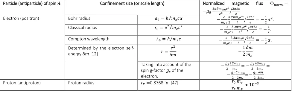
In table I, we summarize such considerations by evaluating the normalized magnetic flux Φ𝑛𝑜𝑟𝑚=
−𝜇𝐵2𝜋𝛿𝑚𝐸𝑀𝑐2 𝑒2
2𝜋ℏ𝑐
𝑒
7
Particle (antiparticle) of spin ½ Confinement size (or scale length) Normalized magnetic flux Φ𝑛𝑜𝑟𝑚=
−𝜇𝐵2𝜋𝛿𝑚𝑒𝑚𝑐 2 𝑒2
2𝜋ℏ𝑐 𝑒
⁄
Electron (positron) Bohr radius 𝑎0= ℏ 𝑚⁄ 𝑒𝑐𝛼 − 𝑒
𝑚𝑒𝑐 ℏ 2
2𝜋𝑚𝑒𝑐𝛼 ℏ
2𝜋ℏ𝑐 𝑒
⁄ = −1
2𝛼 2.
Classical radius 𝑟0= 𝑒2⁄𝑚𝑒𝑐2 − 𝑒
𝑚𝑒𝑐 ℏ 2
2𝜋𝑚𝑒𝑐2 𝑒2
2𝜋ℏ𝑐 𝑒
⁄ = −1
2.
Compton wavelength 𝜆0= ℏ 𝑚⁄ 𝑒𝑐 − 𝑒
𝑚𝑒𝑐 ℏ 2
2𝜋𝑚𝑒𝑐 ℏ
2𝜋ℏ𝑐 𝑒
⁄ = −12𝛼.
Determined by the electron
self-energy 𝛿𝑚 [12] 𝑟 =
𝑒2 𝛿𝑚 − 1 2 𝛿𝑚 𝑚𝑒
Taking into account of the spin g-factor 𝑔𝑠 of the
electron. −𝑔𝑠 2 2𝛿𝑚𝑒𝑠 𝑚𝑒 = − 𝑔𝑠 2 4𝛿𝑚𝑒𝑠
2𝑚𝑒 =
−𝑔𝑠 2
𝛿𝑚𝑒𝑚
2𝑚𝑒=−
𝑔𝑠 2
𝛿𝑚 2𝑚𝑒
Proton (antiproton) Proton radius 𝑟𝑃=0.8768 fm [47] 𝑟0
𝑟𝑃
𝑚𝑒 𝑚𝑃≈ 10
−3
Table I. Normalized magnetic flux Φ𝑛𝑜𝑟𝑚= −𝜇𝐵2𝜋𝛿𝑚𝑒𝑚𝑐 2 𝑒2
2𝜋ℏ𝑐 𝑒
⁄ for different scale lengths or confinement sizes of the spin 1/2 particle. Normalization has been done with respect to the quantum flux 2𝜋ℏ𝑐𝑒 . For the case of an electron (positron) different scale lengths can be considered. By taking into account the electron spin g-factor, a variation of the normalized magnetic flux ∆Φ𝑛𝑜𝑟𝑚for an electron flipping from spin up to down is in module equal to |∆𝛷𝑛𝑜𝑟𝑚| = 𝑔𝑠 2 4𝛿𝑚𝑒𝑠 𝑚𝑒 = 𝑔𝑠 2 𝛿𝑚𝑒𝑚 𝑚𝑒 = 𝑔𝑠 2 𝛿𝑚
𝑚𝑒. Such a variation equals unity, if 𝛿𝑚𝑒𝑚= 𝑚𝑒 𝑔𝑠 2
⁄ . Finally for the case of the proton, we consider
that the minimum length scale is determined by the radius of the proton, which, being a composite particle, is determined by its constituent quarks.
In Figure 1, from a to d, a set of schematizations is also reported in order to show the evolution from classical models of the electromagnetic field of the electrons to QED model of the self-interaction of the electron with its own electromagnetic field. In particular, in Fig.1a we report a representation of the lines of force of the electric and magnetic fields that can be deduced from classical electrodynamics considerations [48]. In Fig.1b we report a representation of the main features and properties of an electron at rest, according to quantum mechanics. Along with its charge −𝑒 and its mass at rest 𝑚𝑒, we have to consider the intrinsic angular momentum or spin
8
Fig.1a Representation of the lines of force of the electric
𝐸⃗⃗ and magnetic fields 𝐵⃗⃗ as deduced from classical electrodynamics [47] for a moving charged particle, being 𝑣⃗ the vector velocity.
Fig.1b Representation of the main features of an electron at rest. An electron, even at rest, has a magnetic field which determines a magnetic moment of −𝜇𝐵 (a
Bohr magneton), for an electron with spin up. The associated magnetic flux determined by the electron is independent of the line path and is quantized in units of
Φ(↑) = −2𝜋𝑐ℏ2𝑒 𝛿𝑚𝑒𝑚
𝑚𝑒 .
Fig.1c A Möbius strip can work as an analogical model reproducing the topological properties of a spin ½ particle subject to a 2π rotation. In the specific case, a spin up will turn into a spin down particle, after following the one-sided surface of the strip and rotating of 2π.
9
4. Formulation of an energy scale comparable to the energy at rest of the electron
In the following an application of equation 19 is considered in order to provide a formulation of an energy scale which is comparable to the energy at rest of the electron. As a matter of fact, radiative corrections within the QED theory provide a contribution to the self-energy determination of the electron [12, 13]. Indeed, by opportunely choosing the cut-off energy required in the QED formulation, a value of the self-energy which is comparable with the energy at rest of the electron can be determined. However, concerning the origin of masses, the diversification of lepton masses can be explained by a Yukawa mechanism of coupling of massless charged leptons with the Higgs field that spontaneously breaks the gauge symmetry [12]. If this is the case we should be able to provide an evaluation of the electron mass within a minimal extension of a scheme which takes into account somehow of the electroweak forces.
In this respect, we may observe as in defining the classical radius 𝑟𝑜 of the electron, the mass at rest of the electron is proportional to the fine structure constant 𝛼 , whereas the classical radius of the electron can be associated to the Compton wavelength of a more massive particle whose
mass reads 𝑚𝑒𝑐
2
𝛼 =
ℏ𝑐
𝑟0. If we consider the Barut formula [49] 𝑚𝜇 = 𝑚𝑒+ 𝑚𝑒
3
2𝛼 for the mass of a
muon, being 𝑚𝑒𝑐
2
𝛼 =
ℏ𝑐 𝑟0 =
2
3(𝑚𝜇 − 𝑚𝑒)𝑐2, we can observe as the mass associated to the classical
radius of the electron is of the same order of magnitude of the mass of a muon. In such a way we can provide a value of the mass of the electron in terms of that of a muon. However, usually we do the opposite, namely we express the mass of heavier leptons in term of the lightest lepton mass, the electron.
On the other hand, we can conjecture that the dependence of the mass of the electron on the fine structure constant 𝛼 is reasonable but it may involve a higher power of 𝛼, such as 𝛼2. If this is the case, the 𝛼2 quantity must be multiplied by the mass value of a heavier particle opportunely chosen. Moreover, we can also expect that the unknown equation expressing an energy, should be in a certain way related to standardized expressions of use within the quantum theory among which we can make a choice. In particular, a mass-energy formula that we can consider stems from the atomic theory. In fact, the equation that relates the Bohr energy of the hydrogen energy levels to the mass of the electron has the same dependence on 𝛼2. Moreover, if we want to pursue the determination of a formula for the mass of the electron within a minimal extension scheme which includes quantities appearing in the electroweak theory, we have to consider the possibility that such heavier mass might be related to the masses of the vector bosons mediating the weak force. Let us devise a thought experiment hence. Namely, let us consider a pair
𝑊+𝑊− of charged 𝑊 vector bosons that undergoes a scattering process at very low energy. If
this is the case, neglecting the very short lifetime of such particles, it results that the scattering amplitudes determined by the Coulomb scattering are influenced by the possible bound states determined by the 𝑊+𝑊− system. The energy of such bound states is lowered with respect to
2𝑀𝑊𝑐2 by the Bohr energy determined by the electromagnetic interaction of the 𝑊+𝑊− pair,
resulting, as a first approximation, in a binding energy , 𝐸𝐵 =12𝛼2 𝑀𝑊𝑐
2
2 , of 1.07 𝑀𝑒𝑉. This
10
when both particles are at rest. And indeed, we can say that the energy scale of an electron at rest is comparable to half of the Bohr energy of a 𝑊+𝑊− pair:
𝑚𝑒𝑐2 ≈18𝛼2𝑀𝑊𝑐2. (25)
Moreover, the difference 2∆𝐸 between the Bohr energy 𝐸𝐵 and the electron-positron pair mass,
results of 48.15 keV:
2∆𝐸 =14𝛼2𝑀
𝑊𝑐2− 2𝑚𝑒𝑐2 = 48.15 𝑘𝑒𝑉. (26)
Indicating as 𝛿𝑀𝑊= 2.085 ± 0.042 𝐺𝑒𝑉 [50] the decay width of a charged vector boson,
assuming that 2𝛿𝑀𝑊 is the uncertainty of the mass of the 𝑊+𝑊− pair, it results that:
1
4𝛼
2(2𝛿𝑀
𝑊)𝑐2 = 55.5 ± 1.1 𝑘𝑒𝑉. (27)
In the hypothesis that such a difference turns out from an indetermination on the mass of the charged boson vector 𝑊, we can wright equation (26) as:
∆𝐸 =18𝛼2𝑀
𝑊𝑐2− 𝑚𝑒𝑐2 ≈81𝛼22𝛿𝑀𝑊𝑐2. (28)
Therefore, the error associated with the mismatch of the two energy scales, the mass of the
electron 𝑚𝑒𝑐2and the corrected Bohr energy of a 𝑊+𝑊− pair 18𝛼2(𝑀𝑊− 2𝛿𝑀𝑊)𝑐2 is:
1 −
1
8𝛼2𝑀𝑊𝑐2− 1
8𝛼22𝛿𝑀𝑊𝑐2
𝑚𝑒𝑐2 ≈ 0.7%, (29)
and differs only by 0.7 % from the mass at rest of an electron.
It is also possible to go further in our evaluation. Indeed, we can introduce an angle 𝜃 such that to take into account of the deviation of difference reported in eq. 26 with respect to the quantity calculated in eq. 27 :
1
4𝛼
2(2𝛿𝑀
𝑊)𝑐2𝑐𝑜𝑠𝜃 =14𝛼2𝑀𝑊𝑐2− 2𝑚𝑒𝑐2. (30)
It results that a reckoning of 𝑐𝑜𝑠𝜃 provides a value of 𝜃 which amounts to 𝜃 =
𝑎𝑐𝑜𝑠 (55.5±1.1 𝑘𝑒𝑉48.15 𝑘𝑒𝑉 ) = (29.8 ± 2)°. Such a value is comparable with the Weinberg angle 𝜃𝑊 =
28.1°. In the hypothesis that the angle 𝜃 is the Weinberg angle 𝜃𝑊, we can gain a value for the energy scale that we are evaluating which is even closer to the energy at rest of the mass of the electron:
𝑚𝑒𝑐2 = 18𝛼2𝑀𝑊𝑐2−18𝛼2(2𝛿𝑀𝑊)𝑐2𝑐𝑜𝑠𝜃𝑊 = 0.5106(5) 𝑀𝑒𝑉 (0.08%), (31)
11
correction, we can obtain a value of an energy scale which differs by only 0.04% with respect to the mass at rest of the electron:
𝑚𝑒𝑐2 = 𝑔𝑠
2 (
1
8𝛼
2𝑀
𝑊𝑐2 −18𝛼2(2𝛿𝑀𝑊)𝑐2𝑐𝑜𝑠𝜃𝑊) = 0.5112(5) 𝑀𝑒𝑉 (0.04%). (32)
Figures 2a and 2b sum up, in sketches, what described so far.
Is this what the mass of an electron should look like? Does eq. 32 determines the mass of the electron? Although the advantage of such a formulation is the use of parameters and quantities which are proper of the electroweak theory, in spite of the close value of the calculated energy scale in eq. 32 to the energy at rest of the electron, a skeptic reader might also consider that the previous heuristic reasoning leads only to a fortunate guess of an energy value which is very close to the mass of an electron. As a fact, we cannot exclude that such a conclusion is a pure coincidence arising from the calculation of the Bohr energy of a 𝑊+𝑊−pair. Although of the many clues provided, such as the Bohr energy and its corrections which are very close to the energy at rest of an 𝑒+𝑒−pair, the Bohr radius of the 𝑊+𝑊− system which is comparable to the classical electron radius, a critical point to consider is the appropriate identification of the angle
𝜃. However, independently of the possible implications which are behind eq. 25 and 32, it is sure that eq. 25, a Bohr energy, is the value of an energy scale comparable to the energy scale of an electron at rest which has been formulated by means of the mass 𝑀𝑊 of the 𝑊 particle.
5. Conclusions
In conclusion, by evaluating a gauge-invariant phase factor (that is a Wilson loop) linked to the electromagnetic gauge field 𝐴𝜇 of the particle, namely an electron, a topological quantum interplay between the magnetic flux Φ and the mass has been demonstrated, In particular, it has been shown that, from the phase factor and the quantization of the magnetic flux variations, a relationship between the mass at rest of the electron 𝑚e and its self-energy 𝛿𝑚, arising from
12
Fig.2a A pair of charged 𝑊 vector bosons (𝑊+𝑊−) is considered to survive long enough to arrange a hydrogen-like system. The Bohr’s radius 𝑎0𝑊+𝑊−= 2ℏ
𝛼𝑀𝑊𝑐 of the
system results comparable to the classical radius of the electron 𝑟0 and to the Compton’s
wavelength of the muon.
In particular, the radius of the nth Bohr’s level 𝑟𝑛𝑊+𝑊−= 𝑛2
2ℏ
𝛼𝑀𝑊𝑐 equals
𝑟𝑛𝑊+𝑊− 𝑟0 =
2𝑛2 1 𝛼2
𝑚𝑒
𝑀𝑊 in units of 𝑟0. A radius of 2𝑟0 is
obtained from the Bohr’s levels between n = 2 and n = 3, whereas a radius of 4𝑟0 can be obtained from the Bohr’s levels between n = 4 and n = 5.
Fig.2b. Comparison of the Bohr’s energy scale 𝐸𝐵of a 𝑊+𝑊− pair, working as a hydrogen-like system, with
the energy of an electron-positron pair 2𝑚𝑒𝑐2=
1.02𝑀𝑒𝑉. The energy associated to the nth Bohr’s orbit
with respect to 2𝑀𝑊𝑐2is lowered by the energy
1 2𝑛2𝛼2 𝑀𝑊
𝑐2
2 and differs, with respect to the ground state,
by an energy ∆𝐸 of ∆𝐸 =1
2(1 − 1
𝑛2) 𝛼2 𝑀𝑊
𝑐2 2 . The energy ∆𝐸 associated to the ground state and n = 5 level is ∆𝐸 =2425∙ 1.07𝑀𝑒𝑉 = 1.027 𝑀𝑒𝑉 .
A better approximation can be obtained by introducing an angle 𝜃, such that a projection of the “segment”
1 4𝛼
2(2𝛿𝑀
𝑊)𝑐2, i.e. 14𝛼2(2𝛿𝑀𝑊)𝑐2cos𝜃, on the vertical
axis, equals the difference between (1
4𝛼 2𝑀
𝑊𝑐2− 2𝑚𝑒𝑐2). The evaluation of such an angle provides a
value which is close to the Weinberg angle 𝜃𝑊. By
adopting 𝜃𝑊= 𝜃, we can estimate a value of the
electron mass which differs only by 0.08 % from the measured one. Multiplying such a value by 𝑔𝑠
2 , it
provides a value which differs only by 0.04 %.
W
+W
-𝑎0𝑊+𝑊−≈ 𝑒
2 𝑚𝑒𝑐2≈
ℏ 𝑚𝜇𝑐
13
References
[1] Nakamura, K. et al. Review of Particle Physics. Journal of Physics G: Nuclear and Particle Physics. 3786, 075021-076443 (2010).
[2] Gaillard, M. K., Grannis, P. D. & Sciulli, F. J. The standard model of particle physics. Rev. Mod. Phys.71, 96-111 (1999).
[3] Sze, S. M. & Kwok K. N. Physics of Semiconductor Devices (3rd ed) (John Wiley & Sons, 2006).
[4] Cramer, C. J. Essentials of Computational Chemistry 153–189 (John Wiley & Sons, 2002).
[5] Pavarini, E., Koch, E., van den Brink, J., Sawatzky, G. (Eds). Quantum materials: experiments and theory. Lecture notes of the autumn school on correlated electrons,
https://www.cond-mat.de/events/correl16/manuscripts/correl16.pdf (2016).
[6] Kohn, W. Nobel Lecture: Electronic structure of matter - wave functions and density functionals. Rev. Mod. Phys. 71, 1253–1266 (1999).
[7] Jones, R. O. Density functional theory: Its origins, rise to prominence, and future. Rev. Mod. Phys.87, 897- 923(2015).
[8] Hohenberg, P. & Kohn, W. Inhomogeneous Electron Gas. Phys. Rev. B. 136, 864–871 (1964).
[9] Kohn, W. & Sham, L. J. Self-consistent equations including exchange and correlation effects. Phys. Rev.140, A1133–A1138(1965).
[10] Sasaki, S. Theory of the Integer & Fractional Quantum Hall Effects (Nova Science Publishers, 2016). Preprint at https://arxiv.org/abs/1603.08625 (2016).
[11] Hasnip, P. J. et al. Density functional theory in the solid state. Philos. Trans. A. Mat. Phys. Eng. Sci.372, 20130270 (2014).
[12] Weinberg, S. The Quantum Theory of Fields, Vol. I (Foundations) (Cambridge University Press, 1995).
14
[14] Thomson, J. J. Cathode rays. Philosophical Magazine.44, 293-316 (1897).
[15] Wilczek, F. The enigmatic electron. Nature.498, 31-32 (2013).
[16] Castelvecchi, D. The Strange topology that is reshaping physics. Nature.547, 272–274 (2017).
[17] Haldane, F. D. M., Model for a Quantum Hall effect without Landau levels: condensed-matter realization of the "parity anomaly". Phys. Rev. Lett. 61, 2015-2018 (1988).
[18] Kosterlitz, J. M. & Thouless, D. J. Ordering, metastability and phase transitions in two-dimensional systems. Journal of Physics C: Solid State Physics.6, 1181–1203 (1973).
[19] Bhattacharjee, S.M. Use of Topology in physical problems in Topology and condensed matter physics. Texts and readings in physical sciences, vol 19 (eds Bhattacharjee, S., Mj, M., Bandyopadhyay, A.) (Springer, 2017).
[20] Nash, C. Topology and Physics a historical essay in History of topology (ed. James, I. M.) 359-415 (North Holland, 1999).
[21] Morandi, G. The role of topology in classical and quantum physics in Lecture notes in physics, m7 (Springer-Verlag, 1992).
[22] Nakahara, M. Geometry, Topology and Physics (CRC Press Taylor & Francis group, 2016).
[23] Stanescu, T. D. Introduction to Topological Quantum Matter & Quantum Computation (CRC Press Taylor & Francis group, 2017).
[24] Dirac, P. A. M. Quantised singularities in the electromagnetic field. Proc. Roy. Soc. A. 133,
60-72 (1931).
[25] Shnir, Y. M. Magnetic Monopoles (Springer, 2005).
[26] Aharonov, Y. & Bohm, D. Significance of electromagnetic potentials in quantum theory. Phys. Rev.115, 485–491 (1959).
[27] Berry, M. V. Quantal phase factors accompanying adiabatic changes. Proc. R. Soc. Lond. A.
392, 45-57 (1984).
[28] Euler, L. Commentarii Academiae Petropolitanae 8, 128-140 (1736).
15
Chimie.13, 315-328 (2010).
[30] Chen, G., Wang, X., Li, X. Fundamentals of Complex Networks: Models, Structures and Dynamics (Wiley, 2015).
[31] Parks, R. D. Quantized magnetic flux in superconductors. Science New Series. 146, 1429-1435 (1964).
[32] London, F. Superfluids (John Wiley and Sons, 1950).
[33] Onsager, L. Proceedings of the International Conference on Theoretical Physics, Kyoto & Tokyo. September 1953 (Science Council of Japan Tokyo, 1954).
[34] Deaver, B. S. & Fairbank, W. M. Experimental evidence for quantized flux in superconducting cylinders. Phys. Rev. Lett.7, 43-46 (1961).
[35] Doll, R. & Näbauer, M. Experimental proof of magnetic flux quantization in a superconducting ring. Phys. Rev. Lett. 7, 51-52 (1961).
[36] Laughlin, R. B. Quantized Hall conductivity in two dimensions.Phys. Rev. B.23, 5632 - 5633 (1981).
[37] Avron, J., Osadchy, D., Seiler, R. A topological look at the quantum Hall effect. Physics Today. 56, 38-42 (2003).
[38] Jehle, H. The relationship of flux quantization to charge quantization and the fine structure constant. Int. Journal of Quantum Chemistry. IIS, 373-375 (1968).
[39] Jehle, H. The relationship of flux quantization to charge quantization and the fine structure constant. Int. Journal of Quantum Chemistry. III, 269-287 (1969).
[40] Jehle, H. Relationship of flux quantization to charge quantization and the electromagnetic coupling constant. Phys. Rev. D.3, 306-345 (1971).
[41] Jehle, H. Flux quantization and particle physics. Phys. Rev. D. 6, 441-457 (1972).
[42] Jehle, H. Flux quantization and fractional charges of quarks. Phys. Rev. D.11, 2147-2177 (1975).
[43] Jehle, H. Topological characterization of leptons, quarks and hadrons. Physics Letters B.
16
[44] Saglam, M., Boyacioglu, B.,Saglam, Z., Yilmaz, O. & Wan, K. K. Spin-dependent quantized magnetic flux through the electronic orbits of Dirac hydrogen atom. Preprint at
https://arxiv.org/ftp/physics/papers/0608/0608165.pdf (2006).
[45] Stein, W. D. R. Quantized magnetic flux through the orbits of hydrogen-like atoms within the atomic model of Sommerfeld. Preprint at https://arxiv.org/pdf/1302.6163v1.pdf (2013).
[46] Wilson, K. G. Confinement of quarks. Phys. Rev. D.10, 2445-2459 (1974).
[47] Pohl, R. et al. The size of the proton. Nature. 466, 213–216 (2010)
[48] Jackson, J. D. Classical Electrodynamics (3rd ed.) (John Wiley & Sons, 1999).
[49] Barut, A. O. The mass of the muon. Phys. Lett. B.73, 310-312 (1978).