
Received: April 23, 2019. In Revised Form: June 18, 2019. Accepted: July 22, 2019. Available online: July 24, 2019. http://dx.doi.org/10.1590/1679-78255599
Some Aspects of Numerical Modeling of Steel-Concrete Composite
Beams with Prestressed Tendons
Jorge Luis Palomino Tamayo a*
Marina Iara Francoa
Inácio Benvegnu Morscha
Jean Marie Désira
Alvaro Marcelo Moscoso Wayarb
a Departamento de Engenharia Civil, Escola de Engenharia, Universidade Federal do Rio Grande do Sul, Av. Osvaldo Aranha 99-3o andar, 90035-190, Porto Alegre, RS, Brasil. Email: [email protected], [email protected], [email protected], [email protected] b Departamento de Ingeniería Civil, Escuela de Arquitectura e Ingeniería, Universidad Privada Boliviana, Camino Achocalla km 2.5-Sector Kañuma, La Paz, Bolivia. Email: [email protected]
* Corresponding author
http://dx.doi.org/10.1590/1679-78255599
Abstract
Aspects about the numerical modeling of three-dimensional prestressed steel-concrete composite beams by using the finite element (FE) method are highlighted and commented in this work. Emphasis is given to the numerical treatment of bonded and unbonded tendons. The proposed modeling technique uses curved beam and catenary elements for simulating internal and external tendons, respectively. Other issues such as the constitutive model for shear connectors, steel beam and concrete are also discussed. Several numerical examples with experimental and numerical results are presented. It is encountered that a faster numerical convergence is achieved when the tendon stiffness is included in the overall stiffness of the structure, even when the unbonded internal situation is addressed. Moreover, omitting slipping at the deviator device may lead to inaccurate results in the evaluation of tendon forces for external prestressing. Favourable agreement is encountered for all studied examples.
Keywords
Steel-concrete composite beams, time effects, relaxation, tendon.
1 INTRODUCTION
serviceability limit states. This can be accomplished by using a FE based approach, in which all issues linked to material behavior, such as slipping at the slab-beam interface, concrete cracking, concrete crushing, shear transfer by aggregate interlock, shear failure of connectors, failure of prestressed and ordinary reinforcements, and yielding of the steel beam are incorporated. Furthermore, the high cost of experiments and the difficulty associated to the local measurement can be overpassed with a calibrated FE model.
The literature about prestressing in steel-concrete composite sections is abundant, but particularly test results and numerical modeling of unbonded internal tendons within the RC slab are more limited. On the one hand, in Ayyub et al. (1992a) this issue is addressed by testing a prestressed composite girder, named E in the experiment, which is comprised of six unbonded internal tendons in the RC slab and subjected to a negative flexure. Therein, experimental results are compared with an analytical approach for predicting the ultimate flexural capacity of the girder (Ayyub et al. 1992a,b). Acceptable matching between experimental and analytical results is then found, however no FE study was realized. In El-zohairy et al. (2017), a numerical and parametric FE study is realized in composite beams with internal and external tendons for ultimate loads. Validation with experimental results is provided for external posttensioned composite beams only, but analyses including unbonded and bonded internal tendons are not compared with experimental dataset. On the other hand, studies with bonded tendons are more commomly encountered in the specialized literature. In Ayyub et al. (1992a), also four internally prestressed steel-concrete composite girders with bonded tendons and precast slabs are tested up to ultimate loading. In Dezi et al. (1995), the viscoelastic analysis of prestressed composite beams with adhered tendon are analyzed. Particular attention is paid to the primary and secondary moment effects generated by prestressing and also to the shear force distribution at the slab-beam interface. Concrete shrinkage and cracking effects were disconsidered in that study. Later, Dezi and co-workers (Dezi et al. 1996) presented simplified and general methods for the time-dependent analysis of steel-concrete composite beams with internal bonded tendons in the RC slabs by using the finite difference method. Although shrinkage is included, concrete cracking is still dismissed. In Stojanovic and Kostic (2015) is presented a viscoelastic approach for internally prestressed steel-concrete composite beams by using the slope-deflection method. In Cao et al. (2018), the response of three prestressed steel-concrete composite continuous box beams (non-prestressed, partly prestressed and fully prestressed) are monitored for 420 days under long-term loads. The main finding of the work is that the development of the rate of deflection of prestressed beams is moderately higher than that of the non-prestressed ones, but no numerical study is carried out. In Jiang et al. (2014), an experimental research campaign is done to study the deformational behavior of steel-encased concrete composite beams with prestressed tendons. Unlike usual composite beams, the steel beam is inside the concrete element. The ANSYS software by means of a 3D FE model is used to validate the experimental dataset.
In the case of external prestressing, in El-zohairy et al. (2015) externally posttensioned composite beams are modeled with the commercial package ANSYS, therein good matching between experimental and predicted results is found for ultimate load analyses. The FE model is comprised of eight-node solid finite elements for representing the RC slab and steel beam. Connectors are modeled by coupling beam and spring elements in the axial and shear direction, respectively, whilst external tendons are modeled with commom truss elements. In Abu-Sena et al. (2018), a parametric study is performed for evaluating the effect of geometrical properties on the ultimate bending response of externally prestressed composite beams by using the commercial package ANSYS. The studied parameters include different cases of loading, tendon profiles, and different dimensions of cross sections. In Lou et al. (2016), externally prestressed steel-concrete composite beams are studied for short- and long-term loads by extending a previous planar beam model, which was initially intended for single RC beams (Lou et al. 2013). In Xue et al. (2008), the long-term behavior of an externally prestressed steel-concrete composite beam is studied under service load for one year.
Works related to unbonded internal tendon formulations in single RC elements are also found in the literature. In Lou et al. (2013), a numerical model is developed for analyzing prestressed RC beams for both service and ultimate analyses. A two-node planar beam element coupled with a straight tendon segment is hence used. It is further assumed that friction between the unbonded tendon and the duct is negligible, yielding a constant strain field over the full tendon length. This situation might correspond to a particular case derived from the approach proposed by Figueiras and Povoas (1994), in which the FE formulation of spatial unbonded curved tendons are developed based on equilibrium considerations. In Moreira et al. (2018), a two-node 2D beam element is used to model prestressed RC beams, with the complete tendon modeled by a single polygonal element crimped in a subset of beam elements. Due to lack of compatibility between the tendon and concrete, the strain in the tendon is calculated from the displacements of all associated beam elements.
tendons as well. Bonded tendons are embedded in the in the RC slab, and are totally adhered to the adjacent concrete. Otherwise, unbonded tendons may be positioned internally or externally to the RC slab. Internal unbonded tendons may slip in relation to the surrounded concrete along its entire length, whereas external tendons only slip at deviator devices located along the longitudinal direction of the steel beam. The model is based on the enhacement of a previous model called VIMIS, developed by the authors, and which have served as FE tool for other numerical studies (Tamayo et al. 2015, Dias et al. 2015, and Reginato et al. 2018). The strategy for including internal and external prestressing and some aspects of the numerical modeling of composite beams are then commented in the following sections. Emphasis is given here to the formulation of unbonded internal tendons because it represents a modification recently introduced to improve the FE model capabilities. The code is validated by comparing experimental and numerical results of several examples. In general aspects, the FE model is optimized by using shell finite elements for representing the steel beam and RC slab instead of more computational expensive solid finite elements. It has been proved that the use of shell finite elements provides accurate responses with lower requirements of memory (see e.g., Razaqpur et al. 2012, Liang et al. 2005, Sebastian and McConnel 2000, Baskar et al. 2002, Bujnak and Bouchair 2005). While the previous version is limited to the analysis of composite beams with ordinary reinforcement in the RC slab, now this is enhaced to deal with prestressing. Moreover, catenary elements can better represent curved shapes with fewer elements in relation to commom truss elements for external tendons. The model is able to capture the entire ultimate load response of continuous steel-concrete composite beams and their time-dependent behavior due to concrete creep and shrinkage for serviceability analyses. For this purpose, the short-term elastoplastic model with the long-term algorithm based on the theory of viscoelasticity are coupled (Dias et al. 2015). Concrete creep is taken into consideration using Kelvin’s rheological model through a step by step time incremental procedure. Thus, a complete picture about numerical modeling of prestressed steel-concrete composite beams is delivered in this work.
2 CONSTITUTIVE MODELING
In the next subsections brief comments about the constitutive models used in the FE code for each part of the steel-concrete composite beam are given. For more details the reader is referred to the works of Tamayo et al. (2015), Tamayo and Awruch (2015) and Dias et al. (2015).
2.1 RC slab, steel beam and shear connector
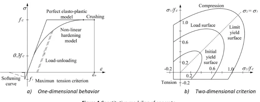
The short-term concrete model is an elastoplastic one, which follows an associated flow rule with nonlinear hardening according to the uniaxial curve depicted in Figure 1(a). In the bidimensional space of principal stresses shown in Figure 1(b), the plastic surface expands from 0,3fc, which is considered to be the limit of the elastic state, to fc,
where fc is the concrete compressive strength. Thereafter, the plastic surface remains constant until finally achieve the
ultimate crushing strain of concrete (0.0035). In this manner, the yield criterion is expressed by means of Equation (1).
𝜎𝜎𝑜𝑜2= 0.355𝜎𝜎𝑜𝑜.�𝜎𝜎𝑥𝑥′+𝜎𝜎𝑦𝑦′�+ 1.355��𝜎𝜎𝑥𝑥′2+𝜎𝜎𝑦𝑦′2 − 𝜎𝜎𝑥𝑥′.𝜎𝜎𝑦𝑦′�+ 3�𝜎𝜎𝑥𝑥′𝑦𝑦′2 +𝜎𝜎𝑥𝑥′𝑧𝑧′2 +𝜎𝜎𝑧𝑧′𝑦𝑦′2 �� (1)
where σo is the effective stress defined by the Madrid parabola as 𝜎𝜎𝑜𝑜=𝐸𝐸𝑐𝑐.�𝜀𝜀̅𝑝𝑝+�2𝜀𝜀𝑜𝑜𝜀𝜀̅𝑝𝑝�, 𝐸𝐸𝑐𝑐 is the Young modulus, 𝜀𝜀̅𝑝𝑝 is the effective plastic strain based on a work hardening hypothesis and 𝜎𝜎𝑖𝑖 with 𝑖𝑖=𝑥𝑥′,𝑦𝑦′,𝑧𝑧′ are the stress components
acting at an arbitrary local system of the RC slab. This criterion is combined with a cut-off criterion for tensile stresses, i.e., concrete in tension is elastic up to it reaches its maximum tensile strength ft. After this value, concrete cracks
Figure 1 Constitutive modeling of concrete.
Otherwise, the multiaxial state of stresses in the steel beam follows the commom Von Mises yield criterion as stated by Equation (2) and shown in Figure 2(a) for the bidimensional space of principal stresses.
𝜎𝜎𝑜𝑜2=𝜎𝜎𝑥𝑥′2 +𝜎𝜎𝑦𝑦′2 − 𝜎𝜎𝑥𝑥′.𝜎𝜎𝑦𝑦′+ 3𝜎𝜎𝑥𝑥′𝑦𝑦′2 (2)
where σo is again the effective stress expressed in terms of the plane stress components 𝜎𝜎𝑥𝑥′, 𝜎𝜎𝑦𝑦′ and 𝜎𝜎𝑥𝑥′𝑦𝑦′. A linear hardening law controlled by the uniaxial curve depicted in Figure 2(b) is futher assumed to monitor the expansion of the plastic surface. This bilinear curve also controls the uniaxial behavior of ordinary and prestressed reinforcements, in which ordinary reinforcement does not creep with time, but relaxation can be induced in the tendon by time effects. Connectors, in charge of transferring shear forces from the RC slab to the steel beam follow a nonlinear law, which relates the current shear force in the connector with the associated slip at the slab-beam interface, as shown Figure 2(c) and defined by Equation (3).
𝐹𝐹𝛽𝛽=𝑎𝑎�1− 𝑒𝑒−𝑏𝑏𝑠𝑠𝛽𝛽� (3)
where 𝐹𝐹𝛽𝛽 and 𝑠𝑠𝛽𝛽 are the shear force in the connector and slip at the slab-beam interface in the 𝛽𝛽 direction,
respectively. When 𝛽𝛽= 90𝑜𝑜, it refers to the shear flow acting along the longitudinal direction of the beam, X-axis in
Figure 3(a). Parameters 𝑎𝑎, 𝑏𝑏 define the ultimate shear force and shape of the connector curve, respectively. They are calibrated in order to match the actual stiffness of the connector encased in a RC slab portion according to 𝑘𝑘𝛽𝛽= 𝑎𝑎𝑏𝑏. exp (−𝑏𝑏𝑠𝑠𝛽𝛽). In this manner, concrete contribution around the connector is taken into consideration in the FE
model. Moreover, slip is computed from the nodal displacement at the conector ends.
2.2 Tendons
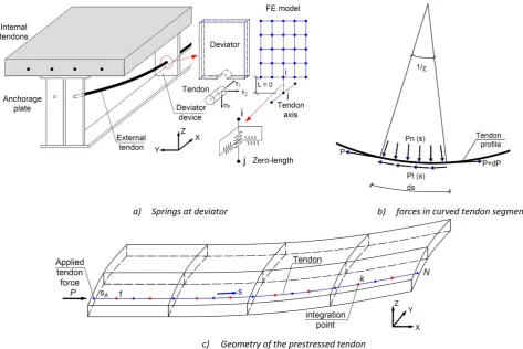
The tension part of the uniaxial stress-strain relationship displayed in Figure 2(b) is also used as a constitutive law for internal and external tendons. The behavior at deviators locations in the case of external prestressing is simulated by using zero-length contact elements, in which slipping between the tendon and a given deviator is allowed along the longitudinal direction (in the axial direction of the tendon segment). Meanwhile, full compatibility is enforced in other directions by using high stiffness values. This release, as it will be shown later, permits obtaining a constant stress field along the tendon length, similar to that encountered in experimental results. Each contact element is composed of three mutually uncoupled perpendicular springs as shown Figure 3(a), where nodes i and j initially share the same nodal coordinates in the undeformed configuration of the beam. Otherwise, in the case of unbonded internal tendons, they are able to slip in relation to the surrounded concrete with some friction. For this purpose, the procedure used by Figueiras and Povoas (1994) is employed herein to compute the strains from nodal displacements. Firstly, the equilibrium condition for a generic curved tendon segment, as shown in Figure 3(b), is stated by means of Equation (4).
𝑑𝑑𝑑𝑑 𝑑𝑑𝑠𝑠
� = ±𝜇𝜇𝜇𝜇𝑑𝑑(𝑠𝑠) (4)
where 𝜇𝜇 and 𝜇𝜇 are the friction coefficient and curvature of a tendon segment of length 𝑑𝑑𝑠𝑠, while 𝑑𝑑(𝑠𝑠) is the associated prestressed force in the tendon at a generic section s. The sign of the equation depends upon the relative movement between the tendon and the sheathing. The solution of the differential equation allows expressing the tendon strain by means of Equation (5) (see Figueiras and Povoas 1994).
Δ𝜀𝜀𝑝𝑝 =Δ𝜀𝜀𝑝𝑝,𝑚𝑚.𝑒𝑒∫ ±𝜇𝜇𝜇𝜇𝜇𝜇𝑠𝑠
𝑠𝑠
𝑠𝑠𝐴𝐴 /𝐸𝐸𝑝𝑝(𝑠𝑠) (5)
with,
Δ𝜀𝜀𝑝𝑝,𝑚𝑚=𝑒𝑒∫ Δ𝜀𝜀𝑙𝑙𝑝𝑝 𝑐𝑐,𝑝𝑝𝜇𝜇𝑠𝑠 (6)
where 𝐸𝐸𝑝𝑝(𝑠𝑠) is the Young modulus of the prestressed steel, Δ𝜀𝜀𝑝𝑝 is the increment of strain in the unbonded tendon, Δ𝜀𝜀𝑐𝑐,𝑝𝑝 is the strain increment in the concrete fiber next to the tendon, and Δ𝜀𝜀𝑝𝑝.𝑚𝑚 is the average strain increment in the
tendon acting along its length. The integrals appearing in Equations (5) and (6) refer to tendon section sA, which corresponds to the anchorage end A, in which the prestressed force is applied, meanwhile s refers to a generic section along the tendon length 𝑙𝑙𝑝𝑝 (see Figure 3(c)). For the particular case when 𝜇𝜇= 0, i.e., when the tendon is straight, as
commonly occurs in RC slabs of composite sections, or when 𝜇𝜇= 0 (i.e., fully unbonded), the strain increment is uniform along the tendon length, Δ𝜀𝜀𝑝𝑝=Δ𝜀𝜀𝑝𝑝,𝑚𝑚. After, Δ𝜀𝜀𝑝𝑝, is computed from Equation (5), the stress increment, Δ𝜎𝜎𝑝𝑝, is
obtained from the current total strain by using the strain-stress relationship shown in Figure 2(b). Therefore, the current stress in the tendon for short-term loads is evaluated by means of Equation (7).
𝜎𝜎𝑝𝑝 =𝜎𝜎𝑝𝑝𝑜𝑜+∆𝜎𝜎𝑝𝑝 (7)
with 𝜎𝜎𝑝𝑝𝑜𝑜 being the previous stress in the tendon. For time effects, the prestress loss increment ∆𝜎𝜎𝑝𝑝𝑝𝑝,𝑟𝑟 due to steel
relaxation must be added to the right hand side of Equation (7). This quantity is computed based on the tendon yield strength 𝑓𝑓𝑝𝑝𝑦𝑦, kind of steel relaxation and time interval, 𝑡𝑡, of interest. The time is measured in hours from the instant at
which the initial prestress, 𝜎𝜎𝑝𝑝𝑜𝑜, is applied. A factor 𝑘𝑘 equal to 10 and 45 is assigned for steels with normal and low
relaxation, respectively.
∆𝜎𝜎𝑝𝑝𝑝𝑝,𝑟𝑟 =−𝜎𝜎𝑘𝑘𝑝𝑝𝑝𝑝�𝑙𝑙𝑙𝑙𝑙𝑙10𝑡𝑡 �𝜎𝜎𝑓𝑓𝑝𝑝𝑝𝑝𝑝𝑝𝑝𝑝−0.55�� (8)
3 FINITE ELEMENT FORMULATIONS
sections. More details can be found in Tamayo et al. (2015) for the RC slab, steel beam and shear connector, meanwhile the reader is refered to the work of Figueiras and Povoas (1994) for the internal tendon element formulation.
3.1 RC slab, steel beam and shear connector
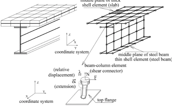
Three-dimensional shell elements with eight nodes are used to represent the middle plane of the RC slab. The slab element is composed of several layers through its thickness in order to properly capture nonlinear variation due to concrete behavior. Additional smeared layers are also defined to represent steel reinforcement as shown in Figure 4(a). The element presents five degrees of freedom at each node with three translation and two in-plane rotations. The FE mesh is established in order to properly capture cracking and crushing at monitored points. Otherwise, the mid-planes of the steel beam, i.e., flanges and web are modeled with four-noded thin shell elements. This element results from the assemblage of a thin plate element with a membrane element with drilling degree of freedom, resulting in an element with six degrees of freedom at each node as displayed in Figure 4(b). The element is able to detect plastic zones by using five integration points through its thickness.
Shear connectors are modeled by means of two-node beam-colum elements as represented in Figure 5, which joint the middle plane of the RC slab with the adjancent middle plane of the upper steel flange at discrete locations, according to the spacing of connectors in the real project. Then, a gap equal to the sum of half slab thickness plus half top flange thickness exists between the slab and the top steel flange of the beam.
Figure 3 Elements used for external and internal prestressing.
• It is assumed that 𝑣𝑣𝑐𝑐𝑚𝑚=𝑣𝑣𝑠𝑠𝑚𝑚, i.e., there is no uplift between the slab and steel beam, where superscript 𝑚𝑚 refers to
the central connector in Figure 6 and subscripts 𝑐𝑐 and 𝑠𝑠 refer to the concrete slab and steel beam, respectively. This compatibility is obtained by using a high axial stiffness in the longitudinal direction of the connector.
• It is assumed that 𝜃𝜃𝑐𝑐𝑚𝑚=𝜃𝜃𝑠𝑠𝑚𝑚, i.e., compatibility of rotations is forced in adjacent nodes based on the assumption
that the beam section remains plane after deformation. This is done by imposing equal rotations on nodes for slab and steel beam.
• The horizontal displacement in each node of the slab with an adjancent connector is computed as the sum of the displacement of the corresponding node on the top steel flange increased by the relative slip in the connector, i.e., 𝑢𝑢𝑐𝑐𝑚𝑚=𝑢𝑢𝑠𝑠𝑚𝑚+𝑠𝑠𝑚𝑚, where the current total slip 𝑠𝑠𝑚𝑚 is computed from the constitutive law shown in Figure 2(c).
Also, a secant version may be used 𝑠𝑠𝑛𝑛𝑚𝑚=𝐹𝐹(𝑠𝑠𝑛𝑛𝑚𝑚)/𝑘𝑘𝑛𝑛𝑚𝑚, where 𝑘𝑘𝑛𝑛𝑚𝑚 is the current secant stiffness of the connector.
Figure 4 Finite element for RC slab and steel beam.
Figure 6 Kinematic assumptions for the shear connection (Bujnak and Bouchair 2005).
3.2 Tendons
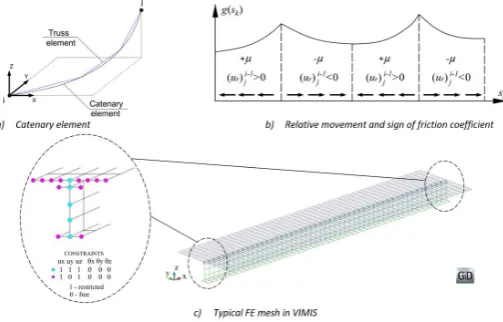
External tendons are modeled using 3D catenary elements as displayed in Figure 7(a), which are accurate because the equilibrium position of a hanging catenary is intrinsic, while they better match curved forms with fewer elements in relation to commom truss elements. Furthermore, this element is appropriate for flexible cables subjected to self-weight loads, and its complete FE formulation can be found elsewhere (Coarita and Flores 2015). The external tendons behave similarly to internally unbonded tendons with full compatibility at anchorage zones, whereas they are attached at discrete locations to deviator devices along its length (Moscoso et al. 2017). At the anchorage zone, the catenary and shell elements representing the tendon and plate, respectively, share the same node in the FE model.
Otherwise, internal bonded or unbonded tendons are simulated by one-dimensional curved elements embedded in the RC slab as shown in Figure 3(c). The algorithm for computing the incremental strain ∆𝜀𝜀𝑝𝑝 stated in Equation (5)
follows the numerical integration presented in the work of Figueiras and Povoas (1994). The method initiates at the anchorage end, designated as section A, and takes in sequence the integration points of all tendon segments. The procedure is explained in the following lines.
1. Calculate the strain in concrete ∆𝜀𝜀𝑐𝑐,𝑝𝑝.
Compute the increment of strain in concrete at the tendon level ∆𝜀𝜀𝑐𝑐,𝑝𝑝 =𝐵𝐵𝑝𝑝.∆𝑑𝑑, in which 𝐵𝐵𝑝𝑝 is the commom
strain-displacement matrix of a curved tendon segment at the current integration point, and ∆𝑑𝑑 is the incremental displacement vector of nodal variables of the slab finite element, in which the current tendon segment is embedded. Calculate ∆𝜀𝜀𝑐𝑐,𝑝𝑝 at each integration point and find the variation in length of the tendon with the following equation.
Δ𝑙𝑙𝑝𝑝 =∑𝑘𝑘=1𝑁𝑁 �Δ𝜀𝜀𝑐𝑐,𝑝𝑝�𝑘𝑘.𝑣𝑣𝑘𝑘.𝑤𝑤𝑘𝑘 (9)
where N is the number of integration points along the tendon, 𝑣𝑣𝑘𝑘 is the norm of a vector tangent to the tendon at the
integration point 𝑘𝑘, and 𝑤𝑤𝑘𝑘 is the associated weight of integration. If the tendon is straight, 𝑣𝑣𝑘𝑘 adopts a unit value. It is
important to mention that a tendon element is formed by various tendon segments along its length. Then, Equation (9) is applied to each tendon embedded in the RC slab.
2. Next, shape function 𝑙𝑙(𝑠𝑠𝑘𝑘) is calculated.
𝑙𝑙(𝑠𝑠𝑘𝑘) =𝑙𝑙𝑘𝑘 =�𝐸𝐸1
𝑝𝑝�𝑘𝑘∏ 𝑒𝑒
±𝜇𝜇𝜇𝜇𝑗𝑗𝑣𝑣𝑗𝑗𝑤𝑤𝑗𝑗
𝑘𝑘
𝑗𝑗=1 (10)
𝑖𝑖𝑡𝑡𝑒𝑒𝑖𝑖𝑎𝑎𝑡𝑡𝑖𝑖𝑙𝑙𝑖𝑖 1: �∆𝜀𝜀𝑐𝑐,𝑝𝑝�1𝑗𝑗− �∆𝜀𝜀𝑐𝑐,𝑝𝑝�𝑗𝑗−11 �
> 0→ 𝑝𝑝𝑙𝑙𝑠𝑠𝑖𝑖𝑡𝑡𝑖𝑖𝑣𝑣𝑒𝑒 𝑠𝑠𝑖𝑖𝑙𝑙𝑖𝑖 < 0→ 𝑖𝑖𝑒𝑒𝑙𝑙𝑎𝑎𝑡𝑡𝑖𝑖𝑣𝑣𝑒𝑒 𝑠𝑠𝑖𝑖𝑙𝑙𝑖𝑖
= 0→ 𝜇𝜇= 0 (11)
𝑖𝑖𝑡𝑡𝑒𝑒𝑖𝑖𝑎𝑎𝑡𝑡𝑖𝑖𝑙𝑙𝑖𝑖 𝑖𝑖> 1: (𝑢𝑢𝑟𝑟)𝑗𝑗𝑖𝑖−1=�𝑢𝑢𝑝𝑝�𝑗𝑗𝑖𝑖−1− �𝑢𝑢𝑐𝑐,𝑝𝑝�𝑗𝑗𝑖𝑖−1 �
> 0→ 𝑝𝑝𝑙𝑙𝑠𝑠𝑖𝑖𝑡𝑡𝑖𝑖𝑣𝑣𝑒𝑒 𝑠𝑠𝑖𝑖𝑙𝑙𝑖𝑖 < 0→ 𝑖𝑖𝑒𝑒𝑙𝑙𝑎𝑎𝑡𝑡𝑖𝑖𝑣𝑣𝑒𝑒 𝑠𝑠𝑖𝑖𝑙𝑙𝑖𝑖
= 0→ 𝜇𝜇= 0 (12)
where 𝑢𝑢𝑝𝑝 and 𝑢𝑢𝑐𝑐 are the accumulated elongation of the tendon and that of the concrete fiber next to it, respectively,
measured from section sA. In this manner, the relative movement, 𝑢𝑢𝑟𝑟 =𝑢𝑢𝑝𝑝− 𝑢𝑢𝑐𝑐, is introduced, and the corresponding
sign of the friction coefficient is then defined. Precisely, in Figure 7(b) is shown the correlation between the sign of 𝜇𝜇
and 𝑢𝑢𝑟𝑟.
𝑢𝑢𝑝𝑝(s) =∫ ∆𝜀𝜀𝑠𝑠𝑠𝑠𝐴𝐴 𝑝𝑝(𝑠𝑠)𝑑𝑑𝑠𝑠 (13)
𝑢𝑢𝑐𝑐,𝑝𝑝(s) =∫ ∆𝜀𝜀𝑠𝑠𝑠𝑠𝐴𝐴 𝑐𝑐,𝑝𝑝(𝑠𝑠)𝑑𝑑𝑠𝑠 (14)
3. Evaluate the integral,
∫ 𝑙𝑙(s)𝑑𝑑𝑠𝑠𝑙𝑙𝑝𝑝 =∑ 𝑣𝑣𝑘𝑘𝑤𝑤𝑘𝑘
�𝐸𝐸𝑝𝑝�𝑘𝑘
𝑁𝑁
𝑘𝑘=1 ∏𝑗𝑗=1𝑘𝑘 𝑒𝑒±𝜇𝜇𝜇𝜇𝑗𝑗𝑣𝑣𝑗𝑗𝑤𝑤𝑗𝑗 (≡ ∑ 𝑙𝑙𝑘𝑘𝑣𝑣𝑘𝑘𝑤𝑤𝑘𝑘) (15)
4. Finally, the strain increment of Equation (5) is expressed by:
�Δ𝜀𝜀𝑝𝑝�𝑘𝑘=𝑙𝑙𝑘𝑘.∑ 𝑔𝑔𝛥𝛥𝑙𝑙𝑘𝑘𝑣𝑣𝑝𝑝𝑘𝑘𝑤𝑤𝑘𝑘 (16)
The strain increment in the above equation is then used to evaluate the tendon stress increment �Δ𝜎𝜎𝑝𝑝�𝑘𝑘
according to the bilinear law shown in Figure 2(b). The aforementioned procedure has been successfully adopted in single RC elements by Figueiras and Povoas (1994) and Fabregat (1988), and now it is used for prestressed slabs in composite beams. The procedure iterates following the iteration loop of the well-known Newton-Rapshon method, until finally achieved the equilibrion condition for the current load increment. The assemblage of all above-mentioned finite elements was schematically depicted in Figure 5, and now the commonly resulting FE mesh together with boundary conditions used in VIMIS are shown in Figure 7(c). In the next sections, a null friction coefficient is used to model fully unbonded behavior as described in the corresponding experimental reports of the given examples. Furthermore, the tendon stiffness contribution of unbonded tendons is included in the analysis for both numerical stability and speed of convergence of the nonlinear algorithm. This issue is verified in the incoming examples.
4 APPLICATIONS
This section presents various examples in which the proposed FE model corroborates varios test results from RC and steel-concrete beam specimens. The complete input data of all examples may be obtained in the quoted references. Comparison is made between numerical predictions and experimental data whenever is possible. Emphasis is given to the evaluation of prestresed forces in the tendons.
4.1 Prestressed beams tested by Guo et al. (2018) and Tao and Du (1985)
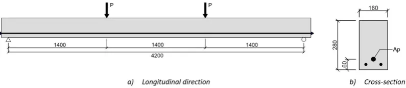
Two prestressed beams with fully unbonded tendons are analyzed in this section. Firstly, beam designated as PC2 tested by Guo et al. (2018), is selected to monitor time dependent prestress losses in the tendon for one year. The curved tendon and beam geometry are displayed in Figure 8. Cubic compressive strength of concrete is 55 MPa. Ordinary steel bars of 12 mm in diameter with steel reinforcement ratio of 0.94%, and yield strength of 335 MPa are used in the beam. The initial prestress force of 103.9 kN is applied at one-end by means of a load cell at 30 days after concrete casting. Immediately after, two point loads of 3.125 kN are applied as a secondary dead load at one-third and two-third points of the span. The tendon has a nominal tensile strength of 1860 MPa and cross section area of 140 mm2.
The second studied beam, designated as A1, is tested by Tao and Du (1985) for ultimate load analysis. This beam is also simply supported and subjected to two point loads as shown in Figure 9. Concrete compressive strength is 30.6 MPa, yield strength of ordinary reinforcement is 267 MPa, concrete crushing strain is 0.0025, and yield and ultimate strengths of the prestressed steel are 1465 MPa and 1790 MPa, respectively. The applied initial prestress is 960 MPa for a tendon area of 58.8 mm2. The beam has a bottom reinforcing steel area of 157 mm2.
Figure 8 Geometry and loading of beam PC2 with curved tendon tested by Guo et al. (2018). [Units: mm]
Figure 9 Geometry and loading of beam A1 with straight tendon tested by Tao and Du (1985). [Units: mm]
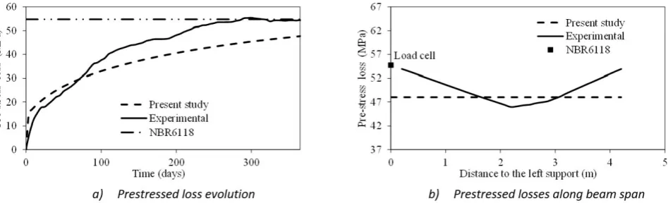
In Figure 10(a) is depicted the prestress loss evolution after jacking for beam PC2 measured at the load cell. As it may be observed, the prestress loss predicted by the FE model slightly underestimates the experimental result with time, but the stress tendency is well established. The predicted final prestress loss is 48 MPa, which represents 6.5% of the initial applied stress; meanwhile this is 53.9 kN (7,3%) in the experiment. Furthermore, the prestress loss predicted according to the formula of the Brazilian Regulation NBR 6118 (2014), which is initially intended for bonded tendons, unexpectantly yielded a closer value of 54.7 MPa (7,4%). Moreover, in Figure 10(b) is depicted the prestres loss evolution along the beam axis. As it can be seen, the experimental prestress loss is higher at the beam ends while it decreases at midspan. Because the tendon is fully unbonded, the numerical model predicts a constant stress field along the tendon length. Reliability studies due to material uncertainties carried out by Chen and Zhang (2018) have demonstrated that the prestress loss in simply supported RC beams can vary substantially in relation to its average value. Hence, the provided FE predictions are in the range of these expected values.
be observed, favourable agreement is also encountered. In Figure 11(c) is displayed the stress tendon evolution with deflection. The ultimate stress value is attained, but the predicted stress path is elastoplastic because a bilinear stress-strain relationship was adopted for the prestressed steel. It is believed that using a multilinear stress-stress-strain relationship would better match the curved experimental stress path. Figure 12(a) depicts the longitudinal normal stresses acting at the upper concrete layer over beam half-span. As expected, the blue zone, which is located between the midspan and a point load, presents the higher compressive stresses. Indeed, the maximum predicted stress is 3.26 kN/cm2, which is slightly higher than the concrete compressive strength of 3.06 kN/cm2. This behavior is verified and illustrated in Figure 12(b) by comparing the experimental and predicted concrete patterns. As it can be seen, cracking spreads from the central region of the beam to the supports from the bottom to the upper layers. Meanwhile, the central region of the upper layer is fully crushed, i.e., concrete losses its rigidity and load resistance capacity, finishing with the overall failure of the beam. Furthermore, a better rate of convergence is attained when the tendon stiffness is included in the numerical analysis
Figure 10 Results of unbonded prestressed beam PC2.
Figure 12 Stresses and cracking patterns for beam A1.
4.2 Long-term analysis of steel-concrete composite beam studied by Dezi et al. (1996)
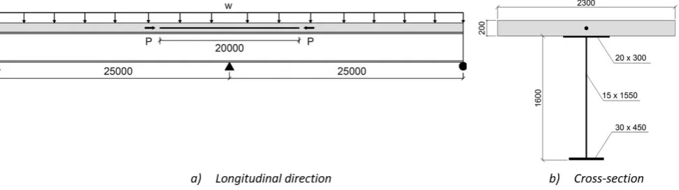
The two-span steel-concrete composite beam shown in Figure 13 is studied in Dezi et al. (1996) for long-term loads. The effects of three applied actions, namely uniformly distributed load of 64.56 kN/m, concrete shrinkage and prestressed force applied to the slab, are evaluated separately in that work. The cross section area of the tendon is 3058 mm2, with a bonded tendon length of 20 m over the interior support, together with a prestressed force of 4000 kN. Concrete compressive strength is 30 MPa, shear connection stiffness is 0.5 kN/mm2 and relative humidity at which the concrete slab was exposured is 50%. All actions are applied at 30 days after concrete casting with shrinkage starting at 7 days. The analysis time is 70 years and the model code CEB-FIP 90 is used for the time-dependent behavior.
Figure 13 Geometry and loading of two-span composite beam studied by Dezi et al. (1996). [Units, mm]
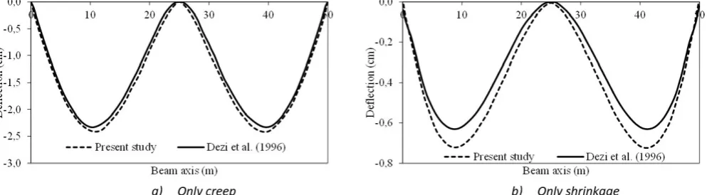
behavior is not able to capture the shear-lag effect. Also, the number of tendons used in the analysis can have a meaningful influence in the final shape of the deflected curves. This is because in Dezi et al.’s model the prestressed force is applied in one tendon along the slab axis. Optionally, in the current FE model, this prestressed force might be applied uniformly in varios tendon elements along the transversal direction of the slab. To better match Dezi et al.’s results, merely one tendon was used in the FE model. It is important to highlight that all the aforementioned effects act together and they cannot be isolated in reality. Although for the current example superposition can be invoked without incurring in too much error.
Figure 14 Deflexion along beam spans after 70 years.
Figure 15 Final values of deflection, tendon force and reaction after 70 years.
4.3 Short-term analysis of steel-concrete composite beam tested by Ayyub et al. (1992a)
spaced in groups of four every 35 cm. The span of the beam is laterally supported to avoid lateral-torsional buckling. Loading is applied in two stages; firstly a prestressed force of 124 kN is applied at each tendon together with the dead load of the beam. Then, a point load is gradually exerted at midspan until failure. Material properties are reported in Ayyub et al. (1992a).
In Figure 17 is displayed the force-deflection curve of the girder at various load levels at midspan. The tested girder failed by buckling of the noncompact compression flange (upper part of the girder at midpan), and the postbuckling prediction is not stable, i.e., the load-deflection curve begins to decline as partially shown in the figure (Ayyub et al. 1992a). Then, its maximum resisting load is nearly the yield load. The predicted load-deflection curve by the FE model, which is based on the nonlinear material response only, correlates well with the measured data at all load levels before local buckling took place. This prediction also partially agrees with the analytical approach presented in Ayyud et al. 1992(b). The cracking load at which the first crack occurs according to Ayyub et al.’s analytical model is 590 kN, while this is 490 kN for the FE model. The yield load, which corresponds to the first yielding of any component of the girder cross section, is 700 kN for the analytical approach and 665 kN for the FE model. The ultimate experimental and numerical loads are virtually the same (700 kN), but a higher ultimate load is forecasted by the analytical approach (955 kN). It is important to establish that the analytical approach is based on equilibrium considerations in the cross section, but it is not able to detect local buckling failure. Although the tendons are totally unbonded, the inclusion of their stiffnesses is crucial for the numerical convergence of the nonlinear algorithm.
To shown futher results, Figures 18(a)-(b) depict the slipping at the slab-beam interface along the span at ultimate load and immediately after pretressing is applied, respectively. As it may be observed, close to the beam ends the slip curve is nearly horizontal acting with their maximum absolute values at these locations, whereas the inflection point with null slip occurs at the point load section. The reported ultimate experimental slip at the beam end is 0.3 mm, while this is 0.8 mm for the FE model.
In Fig. 19 is illustrated the Von Misses stresses in the steel beam at ultimate yield load of 700 kN. As it can be seen, the upper part of the beam at midspan is highly compressed with a maximum stress value of 45.7 kN/cm2, which is higher than the yield strength of the steel beam (38.9 kN/cm2) due to linear hardening of the material. Because of this stress concentration, local buckling is plausible at midspan, but the FE model is not able to detect it. Instead it predicts the yield load and the algorithm is not able to achieve convergence.
Figure 16 Geometry and loading of composite beam tested by Ayyub et al. (1992a). [Units, mm]
Figure 18 Slip over beam span at slab-beam interface.
Figure 19 Von Mises stresses at ultimate load (kN/cm2).
4.4 Short-term analysis of externally prestressed composite beams tested by Nie et al. (2009)
The two-span PCCB4 (fold-line, two-tendon, internal prestressed beam) composite box beam tested in Nie et al. (2009) is selected in this section. Due to symmetry considerations only one half the beam is depicted in Figure 20(a). The cross section is made of a steel box supporting the RC slab as shown in Figure 20(b). The two tendons are anchored at the beam ends and at deviators zones, in which a change of tendons direction occurs. Two point loads are applied symmetrically to each span. Firstly, a prestressed force of 123.22 kN is applied at each tendon, then the two point loads are gradually exerted up to beam failure. The reinforcing bar ratios in the longitudinal and transversal directions are 1.62% and 0.67%, respectively. Concrete compressive strength is 31.4 MPa, the average yield strengths of the steel beam and slab reinforcement are 270 MPa and 300 MPa, respectively. The tendon ultimate strength is 1860 MPa. Shear connectors are 8 mm in diameter, 45 mm in height and spaced in pairs every 80 mm. One tendon area is 139 mm2.
Effect of tendon slipping at the deviators (unbonded case) is compared with its counterpart fully bonded, and load-deflection curves are plotted for this purpose (Figure 21(a)). As it may be observed, the fully bonded and unbonded cases provide nearly similar responses, which also compare well with the experimental data for various load levels, suggesting that slipping of the tendon is not important for the overall response of the composite beam. In Figure 21(b) is depicted the tendon force evolution as loading increases. Along with the experimental results, three curves labeled as Zone1, Zone2 and Zone3 are also plotted for comparison. These zones correspond to tendon segments among deviators and anchorage ends as already defined in Figure 20(a). Each curve defines a diferent stress fields according to its zone. Meanwhile, the unbonded situation predicts a nearly constant stress along its entire length as shown in Figure 22. Then, good matching is found for the tendon force evolution.
Figure 21 Composite beam PCCB4 tested by Nie et al. (2009).
Figure 22 Tendon force (kN) along beam span at ultimate load.
Otherwise, in Figure 23(a) is depicted the predicted cracking pattern at the top concrete layer of the RC slab at service load Pk = 146.76 kN according to the FE model. Due to symmetry considerations only one span is displayed. As it can be seen, flexural cracks represented by blue lines are developed from the interior support up to a distance of 633 mm, i.e., 15.8% of the span length. Meanwhile, compressive stresses represented by red circles are formed between point loads at the positive flexure region. This behavior is similar to that reported in the experimental test at this serviceability stage (Nie et al. 2009). Precisely, in Nie et al.’s work is proposed an equation to predict cracked zone
lengths according to the applied degree of prestressing λ = Mo / Mk in continuous beams, here Mo is the moment
needed to eliminate the compressive stress at the interior support and Mk is the moment at the interior support due to service load Pk, excluding the prestressing effect. The performance of Nie et al.’s formula for various degrees of prestressing is depicted in Figure 23(b). According to this formula, the dimensionless crack length is 13.8% for the
current example (λ = 0.255). This value is very close to 15.8% obtained by the FE analysis. Then, the obtained results
Figure 23 Evaluation of crack length.
5 CONCLUSIONS
In this work, some aspects of the three-dimensional numerical modeling of steel-concrete composite beams with internal and external tendons are presented. For this purpose, a FE model resulting from the assemblage of other model techniques, which were initially intended for single RC elements is proposed. The model is able to deal with all types of nonlinearities of the involved materials as a consequence of the applied short- and long-term loads. Comments and suggestions are then given about the numerical modeling of these structures, in which emphasis is given to the theorical and numerical treatment of strains in unbonded internal tendons. Several examples of single RC specimens and steel-concrete composite beams with experimental dataset and other numerical results, subjected to both service and ultimate loads are reported herein to show model accuracy. Favourable agreement is found in all cases at the global and local level, in which tendon force evolutions are adequately predicted. Thus, the following conclusions can be draw from this study.
In the case of unbonded internal tendons, considering the stiffness of the tendon aims to speed the convergence ratio of the non-linear process and also assures it.
Ommiting slipping at the deviator-tendon interface can lead to innacurate results in the tendon force computation by predicting different stress values among deviator devices. When contact elements are introduced, a uniform tendon force is obtained, which is in accordance with the experimental evidence. However, it seems that the overall response of the structure expressed in terms of load-deflection curves remains unaffected by the inclusion of slipping at the tendon-deviator interface. Then, more examples are needed to generalize this point.
The prediction of local buckling still constitutes a limitation of the current FE model, but work is in progress in order to include its effect by assuming an initially disturbed geometry of the beam. Also, geometric nonlinearility is ongoing.
juxtaposed with deflections from vertical loads, thus indicating a correct implementation of the prestressed tendon formulation in the existing code.
A carefully evaluation of the shear connector stiffness is needed because it has a great influence on the initial slope of the load-deflection curves.
Next steps will include the simulation of the construction process of cable-stayed bridges with steel-concrete composite beams by means of the cantilever method, including time effects. For this purpose, the same catenary element implemented in this work may be used for simulating the supporting cables. Furthermore, the effect of early shrinkage in the RC slab should be also assessed.
Acknowledgment
The financial support provided by CAPES and CNPq is gratefully acknowledged.
Author’s Contributions: Conceptualization, JLP Tamayo and IB Morsch; Methodology, MI Franco and IB Morsch; Investigation, MI Franco; Software, JLP Tamayo, MI Franco and AMM Wayar; Validation, MI Franco, AMM Wayar and JLP Tamayo; Writing-original draft, JLP Tamayo; Writing – review & editing, JM Désir and IB Morsch; Supervision, IB Morsch.
Editor: Pablo Andrés Muñoz Rojas
References
Ayyub, B., Sohn, Y., Saadatmanesh, H. (1992a). Prestressed composite girders. I: Experimental study for negative moment, Journal of Structural Engineering 118: 2743-2762.
Ayyub, B., Sohn, Y., Saadatmanesh, H. (1992b). Prestressed composite girders. II: Analytical study for negative moment, Journal of Structural Engineering 118: 2763-2783.
Abu-Sena, A., Shabaan, I., Soliman, M., Gharib, K. (2018). Effect of geometrical properties on strength of externally prestressed steel-concrete composite beams, Proceedings of the Institution of Civil Engineers – Structures and Buildings,
https://doi.org/10.1680/jstbu.17.00172.
Baskar, K., Shanmugam, N., Thevendran, V. (2002). Finite-element analysis of steel-concrete composite plate girder, Journal of Structural Engineering 128: 1158-1168.
Bujnak, J., Bouchair, A. (2005). Numerical model for steel concrete composite beam with partial shear connection, Proceedings of the European Conference on Steel Structures 4.3: 17-24.
Cao, G., Han, C., Dai, Y., Zhang, W. (2018). Long-term experimental study on prestressed steel-concrete composite continuous box beams, Journal of Bridge Engineering 23: 04018067-1-11.
Coarita, E., Flores, L. (2015). Nonlinear analysis of structures cables-truss, International Journal of Engineering and Technology 7: 160-169.
Chen, Z., Zhang, S. (2018). EM-Based monitoring and probabilistic analysis of prestress loss of bonded tendons in PSC beams, Advances in Civil Engineering 2018: 1-9. https://doi.org/10.1155/2018/4064362.
Dias, M., Tamayo, J., Morsch, I. (2015). Time dependent finite element analysis of steel-concrete composite beams considering partial interaction, Computers and Concrete 15: 687-707.
Dezi, L., Leoni, G., Tarantino, A. (1995). Time dependent analysis of prestressed composite beams, Journal of Structural Engineering 121: 621-633.
Dezi, L., Leoni, G., Tarantino, A. (1996). Algebraic methods for creep analysis of continuous composite beams, Journal of Structural Engineering 122: 423-30.
El-Zohairy, A., Salim, H., Shaaban, H. (2017). Finite element analysis and parametric study of continuos steel-concrete composite beams stiffined with post-tensioned tendons, Advances in Structural Engineering 21:933-945.
Fabregat, P. (1988). Nonlinear model for the analysis of PC plates and shells (in Spanish), Doctoral Thesis, Universidad Politecnica de Catalunya.
Figueiras, J., Póvoas, R. (1994). Modelling of prestress in non-linear analysis of concrete structures, Computers and Concrete 53: 173-187.
Guo, T., Chen, Z., Lu S., Yao R. (2018). Monitoring and analysis of long-term prestress losses in post-tensioned concrete beams, Measurement 122: 573-581.
Jiang, L., Huang, Z., Zhou, W., Xu, X. (2014). Mechanical behavior research of long span prestressed steel-concrete composite beam, Material Research Innovations 18: 28-32.
Liang, Q., Uy, B., Bradford, M., Ronagh, H. (2005). Strength analysis of steel-concrete composite beams in combined bending and shear, Journal of Structural Engineering 131: 1593-1600.
Lou, T., Lopes, S., Lopes, A. (2016). Numerical modeling of externally prestressed steel-concrete composite beams, Journal of Constructional Steel research 121: 229-236.
Lou, T., Lopes, S., Lopes, A. (2013). Nonlinear and time-dependent analysis of continuos unbonded prestressed concrete beams, Computers and Structures 119: 166-176.
Moreira, L., Sousa, J., Parente, E. (2018). Nonlinear finite element simulation of unbounded prestressed concrete beams, Engineering Structures 170: 167-177.
Moscoso, A., Tamayo, J., Morsch, I. (2017). Numerical simulation of external pre-stressed steel-concrete composite beams, Computers and Concrete 19: 191-201.
NBR 6118 (2014). Design of concrete structures-Procedures. Brazilian Association of Technical Regulations. Rio de Janeiro, RJ. Brazil.
Nie, J., Tao, M., Cai, C. S., Li, S. (2009). Deformation analysis of prestressed continuous steel-concrete composite beams, Journal of Structural Engineering 135: 1377-1389.
Razaqpur, G., Nofal, M., Shedid, M., Esfandiari, A. (2012). Nonlinear behavior of steel-concrete composite bridges: finite element modeling and experimental verification, Canadian Journal of Civil Engineering 39: 191-202.
Reginato, L., Tamayo, J., Morsch, I. (2018). Finite element study of effective width in steel-concrete composite beams under long-term service loads, Latin American Journal of Solids and Structures 15: 1-25.
Sebastian, W., McConnel, R. (2000). Nonlinear FE analysis of steel-concrete composite structures, Journal of Structural Engineering 126: 662-674.
Stojanovic, B., Kostic, S. (2015). Time-dependent analysisof composite and prestressed beams using the slope deflection method, Archived of Applied Mechanics 85: 257-272.
Tao, X., Du, G. (1985). Ultimate stress of unbounded tendons in partially prestressed concrete beams, PCI Journal 30: 72-91. Tamayo, J., Awruch, A. (2015). Numerical simulation of reinforced concrete nuclear containment under extreme loads, Structural Engineering and Mechanics 58: 799-823.
Tamayo, J., Morsch, I., Awruch, A. (2015). Short-time numerical analysis of steel-concrete composite beams, Journal of the Brazilian Society of Mechanical Science and Engineering 37: 1097-1109.
Tamayo, J., Morsch, I., Awruch, A. (2013a). Static and dynamic analysis of reinforced concrete shells, Latin American Journal of Solids and Structures 10: 1109-1134.
Tamayo, J., Awruch, A., Morsch, I. (2013b). Numercal modeling of reinforced concrete structures: static and dynamic analysis, REM-Revista Escola de Minas 66: 425-430.

![Figure 16 Geometry and loading of composite beam tested by Ayyub et al. (1992a). [Units, mm]](https://thumb-us.123doks.com/thumbv2/123dok_us/8382936.1679298/14.595.172.407.579.709/figure-geometry-loading-composite-beam-tested-ayyub-units.webp)
