Parameterization of the COM-Poisson Distribution through the Mean Using Spectral Algorithms for Solving Nonlinear Equations

Re-parameterization of the COM-Poisson Distribution Using Spectral

Algorithms

Isaac Adeola Adeniyi

Department of Mathematical Sciences Federal University Lokoja, Nigeria [email protected]

Dolapo Abidemi Shobanke

Department of Mathematical Sciences Federal University Lokoja, Nigeria [email protected]

Helen Olaronke Edogbanya

Department of Mathematical Sciences Federal University Lokoja, Nigeria [email protected]

Abstract

The Poisson regression is popularly used to model count data but real life data often do not satisfy the essential assumption of equality of the mean and variance of the Poisson distribution. The Conway-Maxwell-Poisson (COM-Conway-Maxwell-Poisson) distributions is one of the models that have been proposed for handling cases of over- and under-dispersion. Nevertheless, the parameterization of the COM-Poisson distribution still remains a major challenge in practice as the location parameter of the original COM-Poisson distribution rarely represents the mean of the distribution. As a result, this paper proposes a new parameterization of the COM-Poisson distribution via the central location (mean) so that more easily-interpretable models and results can be obtained. The nonlinear equations resulting from the re-parameterization were solved using the efficient and fast derivative free spectral algorithm. The proposed parameterization is used to present useful numerical results concerning the mean of the COM-Poisson distribution and the location parameter in the original Poisson parameterization. Application of the re-parameterization is further illustrated by fitting COM-Poisson probability models to real life datasets.

Keywords: Count Data; Dispersion Parameter; Overdispersion; Spectral Algorithm; Underdispersion.

MSC: 62E99, 62F99, 62J12, 74S25.

1. Introduction

1983). On the other hand, in cases where the observed variance is less than the mean, it leads to what is referred to as underdispersion. In this case using the Poisson model leads to overestimation of the standard errors and might result to inaccurate inference concerning estimates (Sellers & Shmueli, 2010; Cui et al., 2006).Consequently, the Poisson model despite its simplicity is usually inappropriate and there is need for models which allow wider range of dispersion levels.

Some of the models that have been proposed for handling cases of dispersion where the Poisson model fails include the Negative Binomial (Lawless, 1987; Booth et al, 2003), Generalized Poisson (Famoye, 1993; Cui et al., 2006), Double Poisson (Efron, 1986; Shoukri, 1982; Zou et al., 2013), Hyper-Poisson (Saez-Castillo & Conde-Sanchez, 2013), exponentially-weighted Poisson (Ridout & Besbeas, 2004), the Gamma-count (Zeviani et al., 2014) and the Conway-Maxwell Poisson (COM-Poisson) models (Conway & Maxwell, 1962;Shmueli et al., 2005; Sellers & Shmueli, 2010) amongst others. The Negative Binomial model is popular for handling only overdispersion while both overdispersion and underdispersion can be handled by the Generalized Poisson, Double Poisson, Hyper-Poisson, exponentially-weighted Hyper-Poisson, the Gamma-count model and the Com-Poisson models. Among the methods which can handle underdispersion, the Generalized Poisson and COM-Poisson models have gained wide usage and popularity. Nevertheless, these models still have certain limitations. The Generalized Poisson model can only model a limited degree of underdispersion while the COM-Poisson model has parameterization issues despite having desirable properties such as being a member of the exponential family of distributions; the ability to handle any level of dispersion and being a generalization of important distributions which include the Poisson, Bernoulli and the Geometric distributions.

The Conway-Maxwell-Poisson (COM-Poisson) distribution was developed by Conway and Maxwell (1962) primarily for studying the processes involved in queues. The basic properties of the COM-Poisson distribution were studied by Shmueli et al. (2005). The distribution is a two way parameter extension of the Poisson distribution; it possesses unique properties such that it can effectively fit count data with varying dispersion levels. The probability mass function (PMF) of the COM-Poisson for the discrete count 𝑦, according to Shmueli et al. (2005), is given as:

𝑝(𝑦 ; 𝜆, 𝜈) = 𝜆

𝑦

(𝑦!)𝜈_{𝑍(𝜆, 𝜈)} (1)

where

𝑍(𝜆, 𝜈) = ∑ 𝜆ℎ (ℎ!)𝜈

∞

ℎ=0

𝜆 > 0, 𝜈 ≥ 0, 𝑦 = 0, 1,2, …

From the Probability Mass Function above 𝜆 is the parameter representing the location parameter of the distribution, 𝜈 is the shape parameter while 𝑍 is the normalizing constant. The dispersion parameter 𝜈 = 1 represents equidispersion (Poisson distribution), 𝜈 >

1 represents underdispersion while 𝜈 < 1 refers to overdispersion. According to Shmueli et al. (2005), the mean and variance of the distribution are given by:

𝐸(𝑌) =𝜕 ln(𝑍(𝜆, 𝜈))

𝜕 ln 𝜆 (2) 𝑉𝑎𝑟(𝑌_𝑖) =𝜕²𝑍(𝜆, 𝜈)

The mean and variance of the distribution can also be expressed as

𝐸(𝑌) =𝜆𝜕 ln(𝑍(𝜆, 𝜈))

𝜕𝜆 = ∑

ℎ𝜆𝑖ℎ

𝑍(𝜆, 𝜈)(ℎ!)𝜈

∞

ℎ=0

(4)

and

𝑉𝑎𝑟(𝑌) = 𝐸(𝑌)

𝜕 ln 𝜆 (5)

respectively. Shmueli et al. (2005) used an asymptotic expression to derive an approximation for 𝑍 and gave approximations of the mean and variance as:

𝐸(𝑌) ≈ 𝜆1𝜈+ 1 2𝜈⁄ − 1 2⁄ (6)

𝑉𝑎𝑟(𝑌) ≈ 1 𝜈𝜆

1

𝜈 (7)

Shmueli et al. (2005) noted that these approximations may not be accurate for underdispersed data (𝜈 > 1)orfor values of 𝜆

1

𝜈 < 10_.

A major drawback in the standard Com-Poisson formulation given by (1) is that the location parameter 𝜆 would represent the mean of the distribution only when 𝜈 is equal to one. In situations when 𝜈 is not equal to 1, 𝜆 would no longer represent the mean of the distribution, thereby making the use and interpretation of the COM-Poisson model for modelling overdispersed or underdispersed data less straight forward compared to other competing models like the Poisson, Negative Binomial and Generalized Poisson, since the conditional mean is central to estimation and interpretation in the modelling of count data especially in the regression setting. Some methods of circumventing the problem of parameterization have been proposed. Guikema & Coffelt (2008) proposed a re-parameterization of the COM-Poisson distribution by substituting 𝜃 = 𝜆1 𝜈⁄ to provide a clear centering parameter. Notwithstanding, 𝜃 still doesn’t represent the mean of the distribution and this obscures clear interpretation of estimates in terms of the mean. Parameterization via the approximate mean in (6) was proposed by Dikko et al. (2017). They used the parameterization within the mixed effects models framework to model clustered overdispersed and underdispersed data. Huang (2017) showed how the COM-Poisson regression can be done via the mean although the details on solving the nonlinear equations involved was not mentioned.

In this paper, we present a re-parameterization of the COM-Poisson distribution via the central location (mean) by solving nonlinear system of equations using the derivative-free spectral algorithm (DF-SANE). The motivation behind this approach is to provide a fast technique for fitting COM-Poisson models with easy interpretation as other competing models such as the Poisson, Generalized Poisson and the Negative Binomial distributions while retaining the attractive properties of the standard COM-Poisson distribution. The proposed technique was implemented in R (R Core Team, 2018) and demonstrated to obtain some results regarding the relationship between the parameter 𝜆 and the mean of the COM-Poisson distribution at different dispersion levels. The proposed technique was further used to fit COM-Poisson distribution to four real life datasets. The computation time using the R implementation of our method is also evaluated.

relationship between the parameter 𝜆 and the mean of the COM-Poisson distribution. Concluding remarks are given in section 5 while Proofs are given in the Appendix.

2. Re-Parameterization through the mean

In this section, we introduce a new parameterization of the COM-Poisson distribution. This technique is described as follows. Let the mean of the distribution be expressed as 𝐸(𝑦) =

𝜇, from (2), one can see that 𝜇 is clearly a function of 𝜆 and 𝜈, so 𝜆 is a function of 𝜇 and

𝜈 also. Hence, we set 𝜆 = 𝑔(𝜇) and we express the COM-Poisson PMF as

𝑃(𝑦; 𝜇, 𝜈) = [𝑔(𝜇)]𝑦

(𝑦𝑖!)𝜈𝑍(𝑔(𝜇), 𝜈), 𝜇 > 0, 𝜈 ≥ 0. (8)

Note that 𝜆 is a function of both 𝜇 and 𝜈 but for simplicity’s sake we write 𝑔(𝜇). In this formulation, the PMF is expressed in terms of the mean 𝜇, but to carry out computations using (8) the value of 𝜆 = 𝑔(𝜇) has to be determined. The value of 𝜆 = 𝑔(𝜇) is therefore obtained by solving the following nonlinear equation:

𝜇 −𝜆𝜕 ln(𝑍(𝜆, 𝜈))

𝜕𝜆 = 0. (9)

Equation (9) can also be expressed as

𝜇 − ∑ ℎ𝜆ℎ 𝑍(𝜆, 𝜈)(ℎ!)𝜈

∞

ℎ=0

= 0 (10)

or

∑(𝜇 − ℎ) 𝜆ℎ (ℎ!)𝜈

∞

ℎ=0

= 0. (11)

Given values of 𝜇 and 𝜈 we can solve for the value of 𝜆 and if we have 𝜆 we can solve for

𝜇 from any of the above equations.

One of the useful application of the proposed parameterization is in the estimation of the parameters. Given a random sample 𝑦₁, 𝑦₂, … , 𝑦_𝑛, it can be easily shown that the ML estimator of 𝜇 is the sample mean (see Appendix A), that is, 𝜇̂ = 𝑦̅ =∑ 𝑦𝑖

𝑛 𝑖=1

𝑛 . The sample

mean is easy to calculate, so to obtain the estimate of 𝜆 one just needs to solve (9) with 𝜇 replaced by the sample mean 𝜇̂ = 𝑦̅. Incidentally, the resulting 𝜆̂ is equivalent to the ML estimate of 𝜆 (see Appendix B for proof).

Under the regression setting, this approach allows the modeling of 𝐸(𝑌_𝑖) = 𝜇_𝑖 as a function of covariates 𝑋_𝑖 = [𝑋_𝑖1𝑋_𝑖2 . . . 𝑋_𝑖𝑞] directly instead of through 𝜆. So, the linear predictor of the COM-Poisson generalized linear model using the approach proposed in this study is

𝜇_𝑖 = exp(𝑋_𝑖𝑇_𝛽),

2.1 Estimating 𝝂

Estimating 𝜈 is equally an important task when using the COM-Poisson distribution to model count data. The loglikelihood of the model is given as

𝑙 = ln[𝜆] ∑ 𝑦_𝑖

𝑛

𝑖=1

− 𝜈 ∑ ln 𝑦_𝑖!

𝑛

𝑖=1

− 𝑛 ln[𝑧(𝜆, 𝜈)].

Hence, we propose that 𝜈 be estimated as the solution to the following equation:

∑ ln(𝑦𝑖!)

𝑛 𝑖=1

𝑛 − ∑

ln(ℎ!) 𝑔(𝜇)ℎ

(ℎ!)𝜈_{𝑍(𝑔(𝜇), 𝜈)}

∞

ℎ=0

= 0. (12)

which is obtained by setting _𝜕𝜈𝜕𝑙 = 0. The resulting 𝜈̂ is the maximum likelihood (ML) estimator of 𝜈. Given a random sample 𝑦₁, 𝑦₂, … , 𝑦_𝑛, 𝜇 is replaced with the sample mean

𝑦̅. The values of 𝜆̂ and 𝜈̂ can be obtained simultaneously by solving both (9) and (12) iteratively.

2.2 Solving the Equations

Solutions to equation (9) or any of its equivalents do not exist in closed form expressions and there is need to adopt an iterative nonlinear equation solver. The most common methods for solving equations are the Newton’s method and the Quasi-Newton’s methods (Ortega and Rheinboldt 1970; Dennis and Schnabel 1983). Some modern methods (Bellavia and Morini, 2001; Brown and Saad, 1990; Brown and Saad, 1994; Kelley, 1995) use the Krylov subspace iterative solvers. For this work, we adopt more recent nonlinear equation solvers known as the spectral algorithms (La Cruz and Raydan, 2003; La Cruz et al, 2006; Varadhan and Gilbert, 2009). Brief details on the derivative-free spectral algorithm for solving nonlinear equations (DF-SANE) (La Cruz et al., 2006), which is one of the spectral methods, are given in the next section.

3. Derivative-Free Spectral Algorithm for Solving Nonlinear Equations (DF-SANE)

In the previous section, we present a parameterization of the COM-Poisson distribution via the mean which will lead to solving nonlinear system of equations with no closed form solution. In this section we describe the derivative free spectral algorithm for solving nonlinear equations like (9) and (12) numerically.

Consider a problem of solving the nonlinear system of equation

𝐹(𝑥) = 0, (13)

where 𝐹: ℝ𝑝 → ℝ𝑝is a nonlinear function with continuous partial derivatives. Newton’s method iteratively improves a working linear approximation to F(x) around an estimate of the solution until convergence is achieved and a solution is obtained. The working equation at each iteration is given as

𝑥_𝑘+1 = 𝑥_𝑘 − 𝐽(𝑥_𝑘 )−1 _𝐹(𝑥 𝑘 ),

where 𝐽(𝑥_𝑘 ) is the Jacobian of 𝐹 evaluated at 𝑥_𝑘 . Usually, the Jacobian of 𝐹 is either unavailable or requires a very high amount of computing storage. Quasi-Newton methods replace 𝐽(𝑥_𝑘 ) by suitable approximations but consequently solve a system of linear equation at each iteration which can be computationally expensive.

methods (La Cruz and Raydan, 2003; La Cruz et al, 2006), which are extensions of the Barzilai-Borwein method for finding local minimum (Barzilai and Borwein 1988; Raydan 1997), use ±𝐹(𝑥) as search directions in a systematic way, with one of the spectral coefficients as steplength, and a non-monotone line search technique for global convergence. The algorithm which is robust for solving nonlinear systems is computationally cheap because of the simplicity of search direction and steplength. The spectral approach for solving (13) is defined by the following iteration:

𝑥𝑘+1 = 𝑥𝑘+ 𝛼𝑘𝑑𝑘 , 𝑘 = 0, 1, 2, . .. (14)

where 𝛼𝑘 is the spectral steplength, and 𝑑𝑘 is the search direction. In this work we adopt

the DF-SANE for solving (9) and (12) since it is generally more economical than SANE in terms of number of evaluations of the objective function (Varadhan and Gilbert, 2009), and because it does not require the derivatives of equations (9) and (12), thereby, avoiding the error that would have been incurred as a result of truncating the infinite sums involved in the derivatives. For the derivative free spectral algorithm (DF-SANE), 𝑑𝑘 = −𝐹(𝑥𝑘 ) but

several authors have suggested different methods of calculating the steplength 𝛼𝑘. In our

numerical examples and applications, we use the steplength proposed by Barzilai and Borwein (1988) instead of the one used in the original implementation by La Cruz et al. (2006) because it was found to outperform other alternatives by Varadhan and Gilbert (2009). The steplength we used is defined as

𝛼_𝑘 = 𝑠𝑘−1

𝑇 _𝑦

𝑘−1

𝑦_𝑘−1𝑇 _𝑦 𝑘−1,

where 𝑠_𝑘−1 = 𝑥_𝑘 − 𝑥_𝑘−1 , and 𝑦_𝑘−1= 𝐹(𝑥_𝑘 ) − 𝐹(𝑥_𝑘−1).

Furthermore, following Varadhan and Gilbert (2009), we set 𝛼₀ = min(1, 1 ‖𝐹(𝑥⁄ _𝑘)‖), where ‖∙‖ represents the Euclidian norm, whereas La Cruz et al (2006) used 𝛼₀ = 1. More details on the DF-SANE algorithm are given in La Cruz et al (2006) and Varadhan and Gilbert (2009).The DF-SANE algorithm with the steplength setting described above is implemented by the dfsane function in package BB (Varadhan and Gilbert, 2009) in R (R Core Team, 2018). We take advantage of this implementation of the robust DF-SANE to solve equations (9) and (12) which are classical cases of (13).

4. Applications

The proposed method was implemented in R using the implementation of DF-SANE in the R package BB (Varadhan and Gilbert, 2009) to solve the required nonlinear equations. In this section we show the usefulness of our approach in describing the relationship between

𝜆 and the mean 𝜇. We also used the implementation of our proposal to fit COM-Poisson distributions to real life datasets.

As pointed out earlier, one of the usefulness of our approach is that given values of 𝜇 and

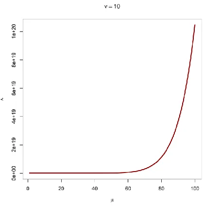
logarithmic. In the case of 𝜈 = 10, the plot suggests that the relationship between 𝜇 and 𝜆 is exponential with the value of 𝜆 increasing faster as 𝜇 increases.

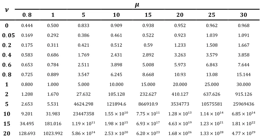
Table 1: Values of 𝜆 for some values of 𝜇 and 𝜈

𝝂 𝝁

𝟎. 𝟖 𝟏 𝟓 𝟏𝟎 𝟏𝟓 𝟐𝟎 𝟐𝟓 𝟑𝟎

𝟎 0.444 0.500 0.833 0.909 0.938 0.952 0.962 0.968

𝟎. 𝟎𝟓 0.169 0.292 0.386 0.461 0.522 0.923 1.039 1.091

𝟎. 𝟐 0.175 0.311 0.421 0.512 0.59 1.233 1.508 1.667

𝟎. 𝟒 0.583 0.686 1.769 2.431 2.892 3.263 3.579 3.858

𝟎. 𝟔 0.653 0.784 2.511 3.898 5.008 5.973 6.843 7.644

𝟎. 𝟖 0.725 0.889 3.547 6.245 8.668 10.93 13.08 15.144

𝟏 0.800 1.000 5.000 10.000 15.000 20.000 25.000 30.000

𝟐 1.208 1.670 27.632 105.128 232.627 410.127 637.626 915.126

𝟓 2.653 5.531 4624.298 121894.6 866910.9 3534773 10575581 25969436

𝟏𝟎 9.201 31.983 23447358 1.55 × 1010 _{7.75 × 10}11 _{1.28 × 10}13 _{1.14 × 10}14 _{6.85 × 10}14 𝟏𝟓 34.495 181.016 1.19 × 1011 _{1.98 × 10}15 _{6.93 × 10}17 _{4.63 × 10}19 _{1.23 × 10}21 _{1.81 × 10}22 𝟐𝟎 128.693 1023.992 5.86 × 1014 _{2.53 × 10}20 _{6.20 × 10}23 _{1.68 × 10}26 _{1.33 × 10}28 _{4.77 × 10}29

Figure 2: Plot of 𝜇 against 𝜆 for 𝜈 = 10

4.1 Application in fitting COM-Poisson Models to Real Life Datasets

To demonstrate the application of the proposed parameterization in fitting COM-Poisson models, we employ four datasets. The first dataset comes from a study that seeks to determine the prevalence of helminths in vegetables sold at the markets of Lokoja, Kogi state, Nigeria. A total of 48 vegetable samples were obtained from the markets over a period of 8 weeks. The second dataset consists of quarterly sales of a well-known brand of a particular article of clothing at stores of a large national retailer used in the paper by Shmueli et al. (2005). The third dataset from Rutherford and Geiger (1910) represent the 2612 counts of number of alpha particles emitted from a source in a given time interval. The fourth dataset consists of numbers of dicentrics per cell for a dose of 1200 radiation in 130 cells from a study by Janardan and Schaffer (1977).

We fitted COM-Poisson models to these datasets using the proposed technique described earlier in sections 2 and 3. The results as well as computational time using a PC with Quadcore 2.4GHz processor and 4 Gigabyte RAM are given in Table 2.

Table 2: Estimates of parameters of the COM-Poisson models for the real life datasets, corresponding goodness of fit test results and computation time

Helminth Sales Alpha Particles Dicentrics

𝝁̂ 1.6458 3.5597 3.8767 4.6538

𝝀̂ 1.1216 0.9748 4.1470 21.9481

𝝂̂ 0.5664 0.1281 1.0452 1.9426

𝝌𝟐

(p value)

16.312

(0.017) (0.6337)19.172 (0.6872)9.902 (0.2204)11.582

Computation time (sec.) 1.44 34.5 7.15 1.54

2.4451 and mean 4.6538 are underdispersed as also indicated by the value of 𝜈̂ (1.9426). The chi-square and p values resulting from goodness of fit tests indicate that the COM-Poisson distribution fits these data well except for the Helminth data which is characterized by a relatively low p value. The results in Table 2 also show that our implementation is quite fast with computations taking few seconds to complete. Our proposal provides an avenue to express the fitted COM-Poisson model in terms of just the sample mean and the estimated dispersion parameter 𝜈̂. For example, the fitted COM-Poisson probability model for the Sales data is given as

𝑃(𝑦_𝑖; 3.6,0.13) = [𝑔(3.6)]𝑦𝑖

(𝑦𝑖!)0.13𝑍(𝑔(3.6), 0.13).

5. Conclusion

The COM-Poisson distribution is well known for its flexibility and robustness in the modelling of dispersed count data. In this paper, we have shown and demonstrated how the COM-Poisson distribution can be parameterized through the mean. One major advantage of this approach is that it allows resulting models to be interpretable easily just like other popular competing distributions like the Poisson and Negative Binomial distribution. The resulting re-parameterized distribution retains all the key properties of the standard COM-Poisson distributions. We adopt the derivative-free spectral algorithm (DF-SANE) for solving the nonlinear equations involved in the parameterization and implemented our approach in R. In addition, we used the implementation of DF-SANE in package BB in R in our implementation.

We used the proposed approach to obtain values of the location parameter in the standard COM-Poisson distribution given various values of the mean and dispersion parameter of the distribution. We further used the approach to fit the COM-Poisson distribution to four real life datasets. We observe that our implementation is quite fast for fitting COM-Poisson distributions to sample data.

Extending this approach to the regression setting is not covered in this paper. Huang (2017) used a similar idea to demonstrate how the COM-Poisson regression can be done via the mean although the method of solving the nonlinear equations involved was not mentioned. Future work could consider fitting COM-Poisson regression models parameterized via the mean using spectral algorithms for solving the nonlinear equations involved. This will facilitate comparing COM-Poisson regression coefficients with those of the Poisson and Negative binomial regressions directly.

Acknowledgments

References

1. Barzilai J. and Borwein J.M. (1988). Two-Point Step Size Gradient Methods. IMA Journal of Numerical Analysis, 8(1), 141–148.

2. Bellavia, S. and Morini, B. (2001). A globally convergent Newton-GMRES subspace method for systems of nonlinear equations. SIAM Journal on Scientific Computing, 23, 940–960.

3. Bohning, D., Dietz E. and Schlattmann P. (1999). The zero-inflated Poisson model and the decayed, missing and filled teeth index in dental epidemiology. Journal of the Royal Statistical Society A, 162, 195–209.

4. Booth, J.G., Casella, G., Friedl, H. and Hobert, J.P. (2003). Negative Binomial Log linear Mixed Models. Statistical Modelling, 3, 179–181.

5. Brown, P. N. and Saad, Y. (1990). Hybrid Krylov methods for nonlinear systems of equations. SIAM Journal on Scientific Computing, 11, 450–481.

6. Consul, P. and Famoye, F. (1988). Maximum Likelihood estimation for the generalized Poisson distribution when sample mean is larger than sample variance.

Communications in Statistics - theory and Methods, 17, 299-309.

7. Conway, R. W. and Maxwell, W. L. (1962). A queuing model with state dependent service rates. Journal of Industrial Engineering, 12, 132–136.

8. Cox, D. R. (1983). Some remarks on overdispersion. Biometrics, 10, 269–274. 9. Cui, Y., Kim, D.Y. and Zhu, J. (2006). On the Generalized Poisson Regression

Mixture Model for Mapping Quantitative Trait Loci with Count Data. Genetics, 174, 2159-2172.

10. Dean C. (1992). Testing for overdispersion in Poisson and binomial regression models. Journal of the American Statistical Association, 87, 451–457.

11. Dennis J. E. and Schnabel R. B. (1983). Numerical Methods for Unconstrained Optimization and Nonlinear Equations. Prentice-Hall, Englewood Cliffs, New Jersey.

12. Dikko, H. G., Asiribo, O. E., Alhaji, B.B. and Shobanke, D. A. (2017). Modelling Underdispersion in Clustered Count Data Using the Modified Conway-Maxwell Poisson Regression. Confluence Journal of Pure and Applied Sciences, 1, 105-130. 13. Efron, B. (1986). Double Exponential Families and Their Use in Generalized Linear Regression. Journal of the American Statistical Association, 81, 709-721. 14. Famoye, F. (1993). Restricted generalized Poisson regression model.

Communications in Statistics - Theory and Methods, 22(5), 1335–1354.

15. Guikema, S. D. and Coffelt, J. P. (2008). A flexible count data regression model for risk analysis. Risk Analysis, 28, 213-223.

16. Huang A. (2017). Mean-parameterized Conway-Maxwell-Poisson regression models for dispersed counts. Statistical Modelling, 17(6): 359-380.

17. Ismail, N. and Jemain, A. A. (2007). Handling Overdispersion with Negative Binomial and Generalized Poisson Regression Models. Casualty Actuarial Society Forum, Winter, 103-158.

18. Janardan, K. K. and Schaeffer, D. J. (1977). Models for the Analysis of Chromosal Aberrations in Human Leukocytes. Biometrical Journal, 19(8), 599-612.

20. La Cruz, W., Martınez J.M. and Raydan M. (2006). “Spectral Residual Method without Gradient Information for Solving Large-Scale Nonlinear Systems of Equations.” Mathematics of Computation, 75(255), 1429.

21. La Cruz, W. and Raydan, M. (2003). “Nonmonotone Spectral Methods for Large-Scale Nonlinear Systems.” Optimization Methods and Software, 18(5), 583–599. 22. Lawless, F. J. (1987). Negative Binomial and Mixed Poisson Regression. The

Canadian Journal of Statistics, 15 (3), 209-225.

23. Ortega, J.M. and Rheinboldt W.C. (1970). Iterative Solution of Non-Linear Equations in Several Variables. Academic Press, New York.

24. Prentice, R. L. (1986). Binary regression using an extended beta-binomial distribution, with discussion of correlation induced by covariate measurement errors. Journal of the American Statistical Association, 81, 321–327.

25. R Core Team (2018). R: A language and environment for statistical computing. R Foundation for Statistical Computing, Vienna, Austria. ISBN 3-900051-07-0, URL https://www.R-project.org/.

26. Raydan M. (1997). “The Barzilai and Borwein Gradient Method for the Large Scale Unconstrained Minimization Problem.” SIAM Journal of Optimization, 7, 26–33. 27. Ridout, M.S. and Besbeas, P. (2004). An empirical model for underdispersed count

data. Statistical Modelling, 4(1), 77–89.

28. Rutherford, E. and Geiger, H. (1910). The Probability Variations in the Distribution of Alpha Particles. Philosophical Magazine, 6 (20), 698-704.

29. Saez-Castillo, A. J. and Conde-Sanchez, A. (2013). A hyper-Poisson regression model for overdispersed and underdispersed count data. Computational Statistics andData Analysis, 61, 148–157.

30. Sellers, K. and Shmueli G. A. (2010). Flexible Regression Model for Count Data.

Annals of Applied Statistics, 4, 943–961. DOI: 10.1214/09-AOAS306.

31. Shmueli, G., Minka, T. P., Kadane, J. B., Borle, S. and Boatwright, P. (2005). A useful distribution for fitting discrete data: revival of the Conway-Maxwell-Poisson distribution. Applied Statistics, 54, 127–142.

32. Shoukri, M. M. (1982). On a Generalisation for the Double Poisson Distribution.

Communication in Statistics – Theory and Methods, 11(2), 151–164.

33. Varadhan, R. and Gilbert, P. (2009). BB: An R Package for Solving a Large System of Nonlinear Equations and for Optimizing a High-Dimensional Nonlinear Objective Function. Journal of Statistical Software, 32(4), 1-26.

34. Zeviani, W. M., Riberio Jr, P. J., Bonat, W. H., Shimakura, S. E. and Muniz, J. A. (2014). The Gamma-count distribution in the analysis of experimental underdispersed data. Journal of Applied Statistics, 41, 2616-2626.

Appendix A: Proof that given sample 𝑦₁, 𝑦₂, … , 𝑦_𝑛, the maximum likelihood estimator of

𝜇 is given as

𝜇̂ = 𝑦̅ =∑ 𝑦𝑖

𝑛 𝑖=1

𝑛 .

The loglikelihood given sample data 𝑦₁, 𝑦₂, … , 𝑦_𝑛 is given as

𝑙 = ln [∏ [𝑔(𝜇)]𝑦𝑖 (𝑦𝑖!)𝜈𝑧(𝑔(𝜇), 𝜈) 𝑛

𝑖=1

]

= ln[𝑔(𝜇)] ∑ 𝑦_𝑖

𝑛

𝑖=1

− 𝜈 ∑ ln 𝑦_𝑖!

𝑛

𝑖=1

− 𝑛 ln[𝑧(𝑔(𝜇), 𝜈)].

Differentiating the loglikelihood 𝑙 with respect to 𝜇 gives

𝜕𝑙 𝜕𝜇 = ( 𝑔′_(𝜇) 𝑔(𝜇)∑ 𝑦𝑖 𝑛 𝑖=1

) − 𝑛𝜕 ln[𝑧(𝑔(𝜇), 𝜈)]

𝜕𝜇 .

Setting _𝜕𝜇𝜕𝑙 = 0 and solving for 𝜇 gives

𝑔(𝜇)𝜕 ln[𝑧(𝑔(𝜇), 𝜈)]

𝑔′_{(𝜇)𝜕𝜇} =

∑𝑛 𝑦_𝑖

𝑖=1

𝑛 . (∗)

Note that 𝑔′(𝜇) =𝑔(𝜇)_𝜕𝜇 , so (∗) becomes

𝑔(𝜇)𝜕 ln[𝑧(𝑔(𝜇), 𝜈)]

𝑔(𝜇) =

∑𝑛 𝑦_𝑖

𝑖=1

𝑛 .

Recall that 𝑔(𝜇) = 𝜆, so we have

𝜆𝜕 ln[𝑧(𝜆, 𝜈)]

𝜆 =

∑𝑛 𝑦_𝑖

𝑖=1

𝑛 .

But 𝜇 =𝜆𝜕 ln[𝑧(𝜆,𝜈)]_𝜆 , so the maximum likelihood estimate of 𝜇 is

𝜇̂ =∑ 𝑦𝑖

𝑛 𝑖=1

𝑛 = 𝑦̅.

Appendix B: Proof that solving (9) with 𝜇 replaced by 𝜇̂ for 𝜆 yields the ML estimate of

𝜆̂.

The loglikelihood given sample data 𝑦₁, 𝑦₂, … , 𝑦_𝑛 is given as

𝑙 = ln[𝜆] ∑ 𝑦_𝑖

𝑛

𝑖=1

− 𝜈 ∑ ln 𝑦_𝑖!

𝑛

𝑖=1

− 𝑛 ln[𝑧(𝜆, 𝜈)]

Differentiating the loglikelihood 𝑙 with respect to 𝜆 gives

𝜕𝑙 𝜕𝜆 = (

∑𝑛 𝑦_𝑖

𝑖=1

𝜆 ) − 𝑛

𝜕 ln[𝑧(𝜆, 𝜈)] 𝜕𝜆

Setting _𝜕𝜆𝜕𝑙 = 0 and solving for 𝜆 gives

𝜆𝜕 ln[𝑧(𝜆, 𝜈)]

𝜕𝜆 =

∑𝑛 𝑦_𝑖

𝑖=1

𝑛 . (∗∗)

But 𝜇̂ =∑ 𝑦𝑖

𝑛 𝑖=1

𝑛 , so (∗∗) becomes

𝜇̂ −𝜆𝜕 ln[𝑧(𝜆, 𝜈)]

𝜕𝜆 = 0. (∗∗∗)

Solving (∗∗∗) for 𝜆 yields the ML estimate of 𝜆 and is the same as (9) with 𝜇 replaced by