Exact reliability formula for a linear consecutive k-out-of-n: F system and relayed consecutive systems with a change point for any

and relayed consecutive systems with a change point for any

𝒌 ≤ 𝒏

, with

stress-strength application

S.M.Bakry

Department of Basic Science

Faculty of Computer and Information Science, Ain Shams University, Cairo, Abbasia, Egypt [email protected]

N.A. Mokhlis

Department of Mathematics

Faculty of Science, Ain Shams University, Cairo, Abbasia, Egypt [email protected]

Abstract

This paper presents exact formulas for the reliability of linear consecutive k-out-of-n: F, and relayed consecutive k-out-of-n: F systems, having a change point at position 𝑐, 1 ≤ 𝑐 ≤ 𝑛, for any 𝑘 ≤ 𝑛. A change point at position 𝑐, means that the components after this point have reliabilities that are different from those before or at position 𝑐. The components are assumed to be independent. Practically, the change in the components reliabilities may be due to change in the stress applied. Assuming a change in stress, exact formulas of the stress-strength reliability of the systems are derived, considering two cases. The first case assumed strength and stress having the same form of distributions, while the second case assumed strength and stress having different forms of distributions. Estimation of the stress-strength reliability for both cases is discussed. Applications to both cases are considered with numerical illustration.

Keywords: Linear (relayed linear) consecutive k-out-of-n: F system; Stress-strength reliability; General exponential form distribution; Generalized Lindley distribution, Maximum likelihood estimator.

Notations

𝑛 Number of components of the system.

𝑘 Minimum number of consecutive failed components required for system failure.

𝑁(𝑗, 𝑠, 𝑟 ) The number of ways in which 𝑗 identical balls can be placed in 𝑠 distinct urns subject to the requirement that at most 𝑟 balls are placed in any one urn.

𝑐 Position of the change point of the system, 1 ≤ 𝑐 ≤ 𝑛.

P Is a vector [𝑝₁, 𝑝₂].

𝐿/𝑘/𝑛/𝑐 Linear consecutive k-out-of-n: F system with a change point at position

𝑐.

𝐿/𝑘/𝑛/𝑐; P 𝐿/𝑘/𝑛/𝑐 with reliability 𝑝1 for components from 1 to 𝑐, and reliability

𝑝₂ from 𝑐 + 1 to 𝑛.

R_w(𝑘, 𝑛, 𝑐; P) Reliability of a 𝐿/𝑘/𝑛/𝑐; P, given that the component at position 𝑐 is working.

R𝐹(𝑘, 𝑛, 𝑐; P) Reliability of a 𝐿/𝑘/𝑛/𝑐; P, given that the component at position 𝑐 is

failed.

R𝑢(𝑘, 𝑛, 𝑐; P) Reliability of a relayed-unipolar 𝐿/𝑘/𝑛/𝑐; P.

R_𝑏(𝑘, 𝑛, 𝑐; P) Reliability of a relayed-bipolar 𝐿/𝑘/𝑛/𝑐; P.

R_(𝑠:𝑠)(𝑘, 𝑛, 𝑐) Stress-strength reliability of a 𝐿/𝑘/𝑛/𝑐.

R_{(𝑠:𝑠)𝑢}(𝑘, 𝑛, 𝑐) Stress-strength reliability of a relayed-unipolar 𝐿/𝑘/𝑛/𝑐.

R_{(𝑠:𝑠)𝑏}(𝑘, 𝑛, 𝑐) Stress-strength reliability of a relayed-bipolar 𝐿/𝑘/𝑛/𝑐.

X, and Stands for a failed, and working component, respectively.

1. Introduction

A linear consecutive k-out-of-n: F system consists of 𝑛 components arranged linearly, the system fails if and only if 𝑘 or more consecutive components fail. There exist many practical applications of this type of systems, for example, the telecommunications system with 𝑛 relay stations, and the oil pipeline system with 𝑛 pump stations, given by Chiang and Niu (1981). Many researches in the literature concerned such systems. Derman et al. (1982) presented a formula for the reliability of a linear consecutive k-out-of-n: F system with identical and independent components with reliabilities 𝑝, given by

R(𝑘, 𝑛; 𝑝) = ∑ 𝑁(𝑗, 𝑛 − 𝑗 + 1, 𝑘 − 1)𝑞𝑗_𝑝𝑛−𝑗 𝑛

𝑗=0

. (1)

Lambiris and Papastavridis (1985) derived an expression for the numbers

𝑁(𝑗, 𝑛 − 𝑗 + 1; 𝑘 − 1) in (1), with 𝑛 − 𝑗 + 1 ≥ 0, as follows

𝑁(𝑗, 𝑛 − 𝑗 + 1, 𝑘 − 1) = ∑ (𝑛 − 𝑗 + 1 𝜆 ) (

𝑛 − 𝜆𝑘

𝑗 − 𝜆𝑘) (−1)𝜆

𝑛−𝑗+1

𝜆=0

. (2)

Other different formulas for the reliability of a linear consecutive k-out-of-n: F system are obtained by different methods, see Chiang and Niu (1981), Hwang (1982), Kossow and Preuss (1989), Ge and Wang (1990), Jung and Kim (1993), Chao et al. (1995), Mokhlis (2001), and Gökdere et al. (2016).

Also, relayed linear consecutive k-out-of-n: F systems are of practical importance. There are two types of relayed linear consecutive k-out-of-n: F systems: The first type is a relayed-unipolar linear consecutive k-out-of-n: F system which is a system consisting of

𝑛 components arranged in a line such that the system fails if the first component fails or at least 𝑘 consecutive components fail; while the second type is a relayed-bipolar linear consecutive k-out-of-n: F system, where the 𝑛 components are arranged in a line such that the system fails if the first or last component fails, or at least 𝑘 consecutive components fail. The notation of relayed-unipolar and bipolar consecutive k out-of-n: F systems is given by Hwang (1988).

multi component stress-strength reliability of consecutive k-out-of-n: G system, for both cases in which there is a change and no change in strength. Zhao et al. (2018) studied a two-stage shock model with self-healing mechanism. A change point is introduced to describe the two-stage failure processes of the system. They proposed three preventive maintenance policies for the system under different monitoring conditions.

Akici (2010) discussed a linear consecutive k-out-of-n: F system with a change point, using the longest run statistic under the condition of special values of 𝑘, 2𝑘 ≥ 𝑛. Akici (2010) mentioned a practical example of this model, which is the gas pipeline from Russia to Turkey. This pipeline system is under two different stresses 𝑋₁ (water) and 𝑋₂ (soil). The pipeline starts from Russia passes across the Black Sea, enter Turkey from Samsun, and ends in Ankara, in Samsun it leaves the sea and enters soil, which is the change point of this system, and there are many other practical examples. Akici (2010) discussed this situation for special values of 𝑘 satisfying 2𝑘 ≥ 𝑛. However, in practice 𝑘 could take any value between 1 and 𝑛, not necessarily, 2𝑘 ≥ 𝑛. So, in this paper we study the reliability of a linear consecutive k-out-of-n: F system with a change point at position

𝑐, when 𝑘 could take any possible value i.e., 1 ≤ 𝑘 ≤ 𝑛. Also, the reliabilities of the relayed-unipolar and relayed-bipolar linear consecutive k-out-of-n: F systems with a change point at position 𝑐 are derived for any 𝑘, 1 ≤ 𝑘 ≤ 𝑛. Exact formulas for the linear and relayed linear (unipolar and bipolar) consecutive k-out-of-n: F systems are derived conditioning on the state (working or failed) of the component at position 𝑐, for any values of 𝑘, 1 ≤ 𝑘 ≤ 𝑛. Formulas for R_(𝑠:𝑠)(𝑘, 𝑛, 𝑐), R_{(𝑠:𝑠)𝑢}(𝑘, 𝑛, 𝑐), and R_{(𝑠:𝑠)𝑏}(𝑘, 𝑛, 𝑐) are derived, for any distributions of strength of components 𝐹(𝑥) and stresses 𝐺_𝑖(𝑥),

𝑖 = 1,2. As application, we discussed two cases: Case I and Case II. Case I, when 𝐹(𝑥) and 𝐺_𝑖(𝑥), 𝑖 = 1,2 have the same form (general exponential form), in this case exact formulas of R_(𝑠:𝑠)(𝑘, 𝑛, 𝑐), R_{(𝑠:𝑠)𝑢}(𝑘, 𝑛, 𝑐), and R_{(𝑠:𝑠)𝑏}(𝑘, 𝑛, 𝑐) are obtained. For illustrating these results numerically, the negative exponential distribution is taken as an example of the general exponential form. Case II, when 𝐹(𝑥) and 𝐺_𝑖(𝑥), 𝑖 = 1,2 have different forms (generalized Lindley distribution for strength and negative exponential distribution for stresses). The Generalized Lindley distribution includes as special cases the exponential, gamma and Lindley distributions, and it is used in stress-strength reliability modeling and analyzing lifetime data, see Elbatal et al. (2013).

The paper is organized as follows: In Section 2, we obtain explicit forms for

R(𝑘, 𝑛, 𝑐; P), R𝑢(𝑘, 𝑛, 𝑐; P), and R𝑏(𝑘, 𝑛, 𝑐; P). In Section 3, we present the

Reliability Formulas

Assume we have a linear consecutive k-out-of-n: F system with independent components, having a change point at position 𝑐. This means that the first 𝑐 components are identical with reliability 𝑝1(𝑞1 = 1 − 𝑝1), while the remaining (𝑛 − 𝑐) components are also

identical but with a different reliability 𝑝₂(𝑞₂ = 1 − 𝑝₂). The reliability of this system,

R(𝑘, 𝑛, 𝑐; P), is given by the following theorem.

Theorem 1

Assuming independent components, for any 𝑘 ≤ 𝑛, and 1 ≤ 𝑐 ≤ 𝑛, we have

R(𝑘, 𝑛, 𝑐; P)

= ∑ 𝑁(𝑚, 𝑐 − 𝑚, 𝑘 − 1)𝑞₁𝑚_𝑝 1𝑐−𝑚 𝑐−1

𝑚=0

× ∑ 𝑁(𝑗 − 𝑚, 𝑛 − 𝑐 − 𝑗 + 𝑚 + 1, 𝑘 − 1)𝑞₂𝑗−𝑚𝑝₂𝑛−𝑐−𝑗+𝑚

𝑛−𝑐+𝑚

𝑗=𝑚

+ ∑ ∑ 𝑁(𝑚 − 𝑟, 𝑐 − 𝑚 − 1, 𝑘 − 1)𝑞₁𝑚+1_𝑝 1𝑐−𝑚−1 𝑐−2

𝑚=𝑟 𝑘−2

𝑟=0

× ∑ ∑ 𝑁(𝑗 − 𝑚 − 𝑤 − 1, 𝑛 − 𝑐 − 𝑗 + 𝑚 + 1, 𝑘 − 1)𝑞₂𝑗−𝑚−1𝑝₂𝑛−𝑐−𝑗+𝑚+1

𝑛−𝑐+𝑚

𝑗=𝑚+𝑤+1 𝑘−𝑟−2

𝑤=0

+𝑞₁𝑐 _{∑ ∑ 𝑁(𝑗 − 𝑐 − 𝑤, 𝑛 − 𝑗, 𝑘 − 1)𝑞}

2𝑗−𝑐𝑝2𝑛−𝑗 𝑛−1

𝑗=𝑐+𝑤 𝑘−𝑐−1

𝑤=0

+𝑞₂𝑛−𝑐 _{∑ ∑ 𝑁(𝑗 − 𝑛 + 𝑐 − 𝑟 − 1, 𝑛 − 𝑗, 𝑘 − 1)𝑞}

1𝑗−𝑛+𝑐𝑝1𝑛−𝑗 𝑛−1

𝑗=𝑛−𝑐+𝑟+1 𝑘−𝑛+𝑐−2

𝑟=0

,

(3)

where ∑ =𝑏_𝑎 0 if 𝑎 > 𝑏, and 𝑁(𝑎, 𝑠, 𝑘 − 1) is computed using Equation (2), take in consideration that (_𝑑𝑏) = 0 if 𝑏, 𝑑 < 0 or 𝑑 > 𝑏.

Proof

The state of the component at position 𝑐 is either working or failed. Conditioning on the state of the component at the change point 𝑐, we have

R(𝑘, 𝑛, 𝑐; P) = 𝑝1R𝑤(𝑘, 𝑛, 𝑐; P) + 𝑞1R𝐹(𝑘, 𝑛, 𝑐; P). (4)

Now, we try to find R_𝑤(𝑘, 𝑛, 𝑐; P) and R_𝐹(𝑘, 𝑛, 𝑐; P). Suppose that we have 𝑗 failed components in the system, 𝑚 failures from these 𝑗 appearing before the change point c, and the remaining 𝑗 − 𝑚 failures appearing after 𝑐.

(i) For computing R_𝑤(𝑘, 𝑛, 𝑐; P) we argue as follows:

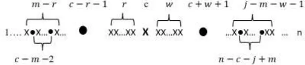
Figure 1: System with 𝑗 failures and the component at position 𝑐 is working.

Figure 1 shows a system with 𝑗 failures, such that 𝑚 failures and 𝑐 − 𝑚 − 1 working components are before c, and 𝑗 − 𝑚 failures and 𝑛 − 𝑐 − 𝑗 + 𝑚 working components are after c. The component at position 𝑐 is operating with reliability 𝑝₁, in this case the position of 𝑐 does not affect the system failure. For the system to operate, we must prevent the appearance of 𝑘 consecutive failures before and after the change point 𝑐. The

𝑚 failures may occupy any position from 1 to 𝑐 − 1, with no consecutive 𝑘 failures, and this can be done by 𝑁(𝑚, 𝑐 − 𝑚, 𝑘 − 1) ways. The remaining 𝑗 − 𝑚 failures may occupy

any position from 𝑐 + 1 to 𝑛 with no consecutive 𝑘 failures, with

𝑁(𝑗 − 𝑚, 𝑛 − 𝑐 − 𝑗 + 𝑚 + 1, 𝑘 − 1) ways. For each 𝑚, each arrangement has probability

𝑞₁𝑚_𝑝

1𝑐−𝑚−1 before the change point 𝑐, and probability 𝑞2𝑗−𝑚𝑝2𝑛−𝑐−𝑗+𝑚 after 𝑐. This means

that

R_w(𝑘, 𝑛, 𝑐; P) = ∑ 𝑁(𝑚, 𝑐 − 𝑚, 𝑘 − 1)

𝑐−1

𝑚=0

𝑞₁𝑚_𝑝 1𝑐−𝑚−1

× ∑ 𝑁(𝑗 − 𝑚, 𝑛 − 𝑐 − 𝑗 + 𝑚 + 1, 𝑘 − 1)𝑞₂𝑗−𝑚𝑝₂𝑛−𝑐−𝑗+𝑚

𝑛−𝑐+𝑚

𝑗=𝑚

.

(5)

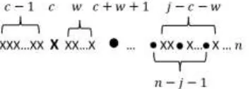
(ii) For computing R𝐹(𝑘, 𝑛, 𝑐; P), we argue as follows:

The component at position 𝑐 fails with probability of failure 𝑞₁, in this case the position of 𝑐 affects the system failure. Then we have the following three cases for the system to operate:

(a) 𝑟 failures from the 𝑚 failures before 𝑐 are directly located before the position 𝑐, and 𝑤 failures from the 𝑗 − 𝑚 failures after 𝑐, are directly located after 𝑐, this situation is depicted by Figure 2, this case for any position of 𝑐, and

1 ≤ 𝑗 ≤ 𝑛 − 2.

Figure 2: System with 𝑗 failures and the component at position 𝑐 is failed.

Figure 2 shows a system with 𝑗 failures, where 𝑟 consecutive failures from the 𝑚 failures are directly located before 𝑐, and 𝑤 consecutive failures from the 𝑗 − 𝑚 failures are directly located after 𝑐. The system operates if 𝑟 + 𝑤 + 1 ≤ 𝑘 − 1, in this case 0 ≤ 𝑟 ≤

𝑐 + 𝑤 + 1, we must have a working component. The remaining 𝑚 − 𝑟 and

𝑗 − 𝑚 − 𝑤 − 1 failures can take any positions in the remaining 𝑐 − 𝑟 − 2 and

𝑛 − 𝑐 − 𝑤 − 1 positions, respectively, without 𝑘 consecutive failures, and this can be done by 𝑁(𝑚 − 𝑟, 𝑐 − 𝑚 − 1, 𝑘 − 1) and 𝑁(𝑗 − 𝑚 − 𝑤 − 1, 𝑛 − 𝑐 − 𝑗 + 𝑚 + 1, 𝑘 − 1) arrangements, respectively. Each arrangement has probability 𝑞₁𝑚𝑝₁𝑐−𝑚−1 before the change point 𝑐, and 𝑞₂𝑗−𝑚−1𝑝₂𝑛−𝑐−𝑗+𝑚+1 after 𝑐, with 1 ≤ 𝑗 ≤ 𝑛 − 2. Hence this possibility occurs with probability

∑ ∑ 𝑁(𝑚 − 𝑟, 𝑐 − 𝑚 − 1, 𝑘 − 1)𝑞₁𝑚_𝑝 1𝑐−𝑚−1 𝑐−2

𝑚=𝑟 𝑘−2

𝑟=0

× ∑ ∑ 𝑁(𝑗 − 𝑚 − 𝑤 − 1, 𝑛 − 𝑐 − 𝑗 + 𝑚 + 1, 𝑘 − 1)𝑞₂𝑗−𝑚−1𝑝₂𝑛−𝑐−𝑗+𝑚+1

𝑛−𝑐+𝑚

𝑗=𝑚+𝑤+1 𝑘−𝑟−2

𝑤=0

.

(6)

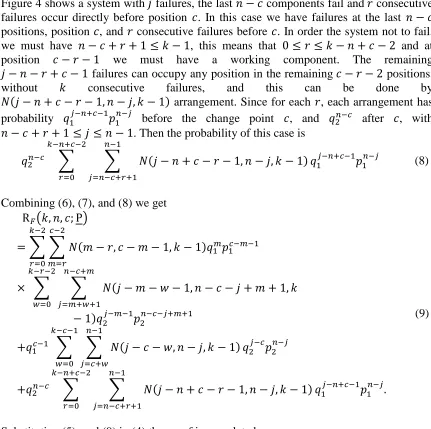
(b) All components before 𝑐 are failures, 𝑐 < 𝑘.

Figure 3: System with 𝑗 failures and the first 𝑐 components failed.

Figure 3 shows a system with 𝑗 failures, the first 𝑐 components failed, and 𝑤 consecutive failures occur directly after those 𝑐 failures. In this case 𝑐 + 𝑤 ≤ 𝑗 ≤ 𝑛 − 1, if 𝑤 of consecutive failures occur directly after the first 𝑐 failed components, then the system operates if 𝑐 + 𝑤 ≤ 𝑘 − 1, then 𝑤 can take values from 0 to 𝑘 − 𝑐 − 1. At position

𝑐 + 𝑤 + 1, we must have a working component. The remaining 𝑗 − 𝑐 − 𝑤 failures can occupy any position in the remaining 𝑛 − 𝑐 − 𝑤 − 1 positions, without 𝑘 consecutive failures. There are 𝑁(𝑗 − 𝑐 − 𝑤, 𝑛 − 𝑗, 𝑘 − 1) arrangements that satisfy the condition. Since for each 𝑤, each arrangement has probability 𝑞₁𝑐−1 before the change point 𝑐, and 𝑞₂𝑗−𝑐𝑝₂𝑛−𝑗 after this point. Then this possibility occurs with probability

𝑞₁𝑐−1 _{∑ ∑ 𝑁(𝑗 − 𝑐 − 𝑤, 𝑛 − 𝑗, 𝑘 − 1)} 𝑛−1

𝑗=𝑐+𝑤

𝑞₂𝑗−𝑐𝑝₂𝑛−𝑗

𝑘−𝑐−1

𝑤=0

. (7)

(c) All components after 𝑐 failed, 𝑐 > 𝑛 − 𝑘 + 1.

Figure 4 shows a system with 𝑗 failures, the last 𝑛 − 𝑐 components fail and 𝑟 consecutive failures occur directly before position 𝑐. In this case we have failures at the last 𝑛 − 𝑐 positions, position 𝑐, and 𝑟 consecutive failures before 𝑐. In order the system not to fail, we must have 𝑛 − 𝑐 + 𝑟 + 1 ≤ 𝑘 − 1, this means that 0 ≤ 𝑟 ≤ 𝑘 − 𝑛 + 𝑐 − 2 and at position 𝑐 − 𝑟 − 1 we must have a working component. The remaining

𝑗 − 𝑛 − 𝑟 + 𝑐 − 1 failures can occupy any position in the remaining 𝑐 − 𝑟 − 2 positions,

without 𝑘 consecutive failures, and this can be done by

𝑁(𝑗 − 𝑛 + 𝑐 − 𝑟 − 1, 𝑛 − 𝑗, 𝑘 − 1) arrangement. Since for each 𝑟, each arrangement has probability 𝑞₁𝑗−𝑛+𝑐−1𝑝₁𝑛−𝑗 before the change point 𝑐, and 𝑞₂𝑛−𝑐 after 𝑐, with

𝑛 − 𝑐 + 𝑟 + 1 ≤ 𝑗 ≤ 𝑛 − 1. Then the probability of this case is

𝑞₂𝑛−𝑐 _{∑ ∑ 𝑁(𝑗 − 𝑛 + 𝑐 − 𝑟 − 1, 𝑛 − 𝑗, 𝑘 − 1)} 𝑛−1

𝑗=𝑛−𝑐+𝑟+1

𝑞₁𝑗−𝑛+𝑐−1𝑝₁𝑛−𝑗

𝑘−𝑛+𝑐−2

𝑟=0

(8)

Combining (6), (7), and (8) we get

R_𝐹(𝑘, 𝑛, 𝑐; P)

= ∑ ∑ 𝑁(𝑚 − 𝑟, 𝑐 − 𝑚 − 1, 𝑘 − 1)𝑞₁𝑚_𝑝 1𝑐−𝑚−1 𝑐−2

𝑚=𝑟 𝑘−2

𝑟=0

× ∑ ∑ 𝑁(𝑗 − 𝑚 − 𝑤 − 1, 𝑛 − 𝑐 − 𝑗 + 𝑚 + 1, 𝑘

𝑛−𝑐+𝑚

𝑗=𝑚+𝑤+1 𝑘−𝑟−2

𝑤=0

− 1)𝑞₂𝑗−𝑚−1𝑝₂𝑛−𝑐−𝑗+𝑚+1

+𝑞₁𝑐−1 _{∑ ∑ 𝑁(𝑗 − 𝑐 − 𝑤, 𝑛 − 𝑗, 𝑘 − 1)} 𝑛−1

𝑗=𝑐+𝑤

𝑞₂𝑗−𝑐𝑝₂𝑛−𝑗

𝑘−𝑐−1

𝑤=0

+𝑞₂𝑛−𝑐 _{∑ ∑ 𝑁(𝑗 − 𝑛 + 𝑐 − 𝑟 − 1, 𝑛 − 𝑗, 𝑘 − 1)} 𝑛−1

𝑗=𝑛−𝑐+𝑟+1

𝑞₁𝑗−𝑛+𝑐−1𝑝₁𝑛−𝑗

𝑘−𝑛+𝑐−2

𝑟=0

.

(9)

Substituting (5), and (9) in (4) the proof is completed.

The following corollary presents the formulas of R_𝑢(𝑘, 𝑛, 𝑐; P) and R_𝑏(𝑘, 𝑛, 𝑐; P).

Corollary 1.

Assuming independent components, for any 𝑘 ≤ 𝑛, 1 ≤ 𝑐 ≤ 𝑛 we have

R_𝑢(𝑘, 𝑛, 𝑐; P) = 𝑝₁R(𝑘, 𝑛 − 1, 𝑐 − 1; P), and (10)

R_𝑏(𝑘, 𝑛, 𝑐; P) = 𝑝₁𝑝₂R(𝑘, 𝑛 − 2, 𝑐 − 1; P). (11)

Remark.

Substituting with 𝑐 = 𝑛and 𝑝1 = 𝑝, 𝑞1 = 𝑞 in (3), we obtain the same result as (1) which

is the result obtained by Derman et al. (1982) for consecutive k-out-of-n: F system without change point. Similarly substituting with 𝑐 = 0 and 𝑝₂ = 𝑝, 𝑞₂ = 𝑞 in (3), we obtain (1). Clearly (1) can be written as

R(𝑘, 𝑛; 𝑝) = ∑ 𝑎_𝑛,𝑗 𝑝𝑗_𝑞𝑛−𝑗 𝑛−1

𝑗=0

, where 𝑎_𝑛,𝑗 = {( 𝑛

Note that if 𝑗 = 𝑛 in (1), the term 𝑁(𝑛, 1, 𝑘 − 1) = 0, for any 𝑘.

Stress-Strength Reliability

In this section we obtain R_(𝑠:𝑠)(𝑘, 𝑛, 𝑐), R_{(𝑠:𝑠)𝑢}(𝑘, 𝑛, 𝑐), and R_{(𝑠:𝑠)𝑏}(𝑘, 𝑛, 𝑐). Suppose that a change in the stress occurs after the component at position 𝑐. Thus, assume we have two common independent stresses 𝑋_𝑖, 𝑖 = 1,2, with cumulative distribution functions

𝐺_𝑖(𝑥), 𝑖 = 1,2, where the common stress 𝑋₁ is imposed on components 1 to 𝑐, and the common stress 𝑋₂ is imposed on components 𝑐 + 1 to 𝑛. The strengths 𝑌_𝑖, 𝑖 = 1, … , 𝑛 of the components are independent and identically distributed, having cumulative distribution function 𝐹(𝑥). The stress-strength reliability of 𝐿/𝑘/𝑛/𝑐 is given by the following theorem.

Theorem 2.

Let 𝐺_𝑖(𝑥), 𝑖 = 1,2 denote the cumulative distribution functions of stresses 𝑋_𝑖, 𝑖 = 1,2, and

𝐹(𝑥) denote the cumulative distribution function of strengths 𝑌_𝑖, 𝑖 = 1, … , 𝑛. Assume that

𝑋1 and 𝑋2 are independent, and 𝑌𝑖′𝑠 are independent and identically distributed. The

stress-strength reliability of 𝐿/𝑘/𝑛/𝑐, for any 𝑘 ≤ 𝑛, and 1 ≤ 𝑐 ≤ 𝑛, is given by

R_(𝑠:𝑠)(𝑘, 𝑛, 𝑐)

= ∑ 𝑁(𝑚, 𝑐 − 𝑚, 𝑘 − 1)

𝑐−1

𝑚=0

𝐼_{𝑚,𝑐−𝑚}1

× ∑ 𝑁(𝑗 − 𝑚, 𝑛 − 𝑐 − 𝑗 + 𝑚 + 1, 𝑘 − 1)

𝑛−𝑐+𝑚

𝑗=𝑚

𝐼_{𝑗−𝑚,𝑛−𝑐−𝑗+𝑚}2

+ ∑ ∑ 𝑁(𝑚 − 𝑟, 𝑐 − 𝑚 − 1, 𝑘 − 1)

𝑐−2

𝑚=𝑟 𝑘−2

𝑟=0

𝐼_{𝑚+1,𝑐−𝑚−1}1

× ∑ ∑ 𝑁(𝑗 − 𝑚 − 𝑤 − 1, 𝑛 − 𝑐 − 𝑗 + 𝑚 + 1, 𝑘 − 1)𝐼_{𝑗−𝑚−1,𝑛−𝑐−𝑗+𝑚+1}2

𝑛−𝑐+𝑚

𝑗=𝑚+𝑤+1 𝑘−𝑟−2

𝑤=0

+𝐼_𝑐,01 _{∑ ∑ 𝑁(𝑗 − 𝑐 − 𝑤, 𝑛 − 𝑗, 𝑘 − 1) 𝐼} 𝑗−𝑐,𝑛−𝑗2 𝑛−1

𝑗=𝑐+𝑤 𝑘−𝑐−1

𝑤=0

+𝐼_{𝑛−𝑐,0}2 _{∑ ∑ 𝑁(𝑗 − 𝑛 + 𝑐 − 𝑟 − 1, 𝑛 − 𝑗, 𝑘 − 1)𝐼}

𝑗−𝑛+𝑐,𝑛−𝑗1 𝑛−1

𝑗=𝑛−𝑐+𝑟+1 𝑘−𝑛+𝑐−2

𝑟=0

,

(12)

where

𝐼_𝑎,𝑏𝑖 _{= ∫ [𝐹(𝑥)]}𝑎_{[1 − 𝐹(𝑥)]}𝑏_𝑑𝐺 𝑖(𝑥) ∞

0

, 𝑖 = 1,2. ₍₁₃₎

Proof

We can easily show that (12) could be obtained by substituting 𝑞_𝑖𝑠𝑝_𝑖ℎ−𝑠 in (3) by

∫ [𝐹(𝑥)]𝑠[1 − 𝐹(𝑥)]ℎ−𝑠_𝑑𝐺 𝑖(𝑥) ∞

ℎ = { _{𝑛 − 𝑐 with 𝑠 = 𝑗 − 𝑚, 𝑗 − 𝑚 − 1, 𝑗 − 𝑐, or 𝑛 − 𝑐 if 𝑖 = 2.}𝑐 with 𝑠 = 𝑚, 𝑚 + 1, 𝑐, or 𝑗 − 𝑛 + 𝑐 if 𝑖 = 1

Corollary 2

Let 𝑋₁ and 𝑋₂ be two common stresses with cumulative distribution functions

𝐺1(𝑥) and 𝐺2(𝑥), imposed on components 1 to 𝑐 and components 𝑐 + 1 to 𝑛,

respectively. Assume that 𝑋1 and 𝑋2 are independent. Let 𝑌𝑖, 𝑖 = 1, … , 𝑛 denote the

strengths of components 1, … , 𝑛. Assume that 𝑌_𝑖′𝑠 are independent and identically distributed. For any 𝑘 ≤ 𝑛, and 1 ≤ 𝑐 ≤ 𝑛, the stress-strength reliability of a unipolar-relayed and bipolar-unipolar-relayed 𝐿/𝑘/𝑛/𝑐 system, is given respectively by

R(𝑠:𝑠)𝑢(𝑘, 𝑛, 𝑐)

= ∑ 𝑁(𝑚, 𝑐 − 𝑚 − 1, 𝑘 − 1)

𝑐−2

𝑚=0

𝐼_{𝑚,𝑐−𝑚}1

× ∑ 𝑁(𝑗 − 𝑚, 𝑛 − 𝑐 − 𝑗 + 𝑚 + 1, 𝑘 − 1)𝐼_{𝑗−𝑚,𝑛−𝑐−𝑗+𝑚}2 𝑛−𝑐+𝑚

𝑗=𝑚

+ ∑ ∑ 𝑁(𝑚 − 𝑟, 𝑐 − 𝑚 − 2, 𝑘 − 1)𝐼𝑚+1,𝑐−𝑚−11 𝑐−3

𝑚=𝑟 𝑘−2

𝑟=0

× ∑ ∑ 𝑁(𝑗 − 𝑚 − 𝑤 − 1, 𝑛 − 𝑐 − 𝑗 + 𝑚 + 1, 𝑘 − 1)𝐼_{𝑗−𝑚−1,𝑛−𝑐−𝑗+𝑚+1}2

𝑛−𝑐+𝑚

𝑗=𝑚+𝑤+1 𝑘−𝑟−2

𝑤=0

+𝐼_𝑐−1,11 _{∑ ∑ 𝑁(𝑗 − 𝑐 − 𝑤 + 1, 𝑛 − 𝑗 − 1, 𝑘 − 1) 𝐼}

𝑗−𝑐+1,𝑛−𝑗−12 𝑛−2

𝑗=𝑐+𝑤−1 𝑘−𝑐

𝑤=0

+ 𝐼_{𝑛−𝑐,0}2 _{∑ ∑ 𝑁(𝑗 − 𝑛 + 𝑐 − 𝑟 − 1, 𝑛 − 𝑗 − 1, 𝑘 − 1)𝐼}

𝑗−𝑛+𝑐,𝑛−𝑗1 𝑛−2

𝑗=𝑛−𝑐+𝑟+1 𝑘−𝑛+𝑐−2

𝑟=0

,

(14)

and

R_{(𝑠:𝑠)𝑏}(𝑘, 𝑛, 𝑐)

= ∑ 𝑁(𝑚, 𝑐 − 𝑚 − 1, 𝑘 − 1)

𝑐−2

𝑚=0

𝐼𝑚,𝑐−𝑚1

× ∑ 𝑁(𝑗 − 𝑚, 𝑛 − 𝑐 − 𝑗 + 𝑚, 𝑘 − 1)𝐼_{𝑗−𝑚,𝑛−𝑐−𝑗+𝑚}2 𝑛−𝑐+𝑚−1

𝑗=𝑚

+ ∑ ∑ 𝑁(𝑚 − 𝑟, 𝑐 − 𝑚 − 2, 𝑘 − 1)𝐼_{𝑚+1,𝑐−𝑚−1}1 𝑐−3

𝑚=𝑟 𝑘−2

𝑟=0

× ∑ ∑ 𝑁(𝑗 − 𝑚 − 𝑤 − 1, 𝑛 − 𝑐 − 𝑗 + 𝑚, 𝑘 − 1)𝐼_{𝑗−𝑚−1,𝑛−𝑐−𝑗+𝑚+1}2

𝑛−𝑐+𝑚−1

𝑗=𝑚+𝑤+1 𝑘−𝑟−2

𝑤=0

+𝐼_𝑐−1,11 _{∑ ∑ 𝑁(𝑗 − 𝑐 − 𝑤 + 1, 𝑛 − 𝑗 − 2, 𝑘 − 1)𝐼}

𝑗−𝑐+1,𝑛−𝑗−12 𝑛−3

𝑗=𝑐+𝑤−1 𝑘−𝑐

𝑤=0

+𝐼_{𝑛−𝑐−1,1}2 _{∑ ∑ 𝑁(𝑗 − 𝑛 + 𝑐 − 𝑟, 𝑛 − 𝑗 − 2, 𝑘 − 1)} 𝑛−3

𝑗=𝑛−𝑐+𝑟 𝑘−𝑛+𝑐−1

𝑟=0

𝐼_{𝑗−𝑛+𝑐+1,𝑛−𝑗−1}1 _.

The Exact Stress-Strength Reliability Formulas for Some Special Distributions

The exact reliability formulas of R_(𝑠:𝑠)(𝑘, 𝑛, 𝑐), R_{(𝑠:𝑠)𝑢}(𝑘, 𝑛, 𝑐), and R_{(𝑠:𝑠)𝑏}(𝑘, 𝑛, 𝑐) are obtained in two cases: case I, when the strength and the stresses have the same form of distributions. As an application of this case, we consider the general exponential form. Case II, when the strength and the stresses have different forms of distributions, and as application, we consider the generalized Lindley distribution for strength, while the stresses have a negative exponential distribution.

Case I

Al-Hussaini (1999) has proposed that survival function 𝐹_𝑋 of any continuous random variable can be expressed by the form 𝐹_𝑋(𝑥) = 𝑒−𝜆(𝑥,𝜃), where 𝜃 could be a vector parameter, 𝜆(𝑥, 𝜃) is a continuous, monotone increasing, and differentiable function such that 𝜆(𝑥, 𝜃) → 0 as 𝑥 → −∞ and 𝜆(𝑥, 𝜃) → ∞ as 𝑥 → ∞. Here we shall consider

𝜆(𝑥, 𝜃) = 𝛿𝑔(𝑥, 𝜗), 𝛿 > 0, 𝑔(𝑥, 𝜗) does not contain 𝛿, and 𝑔(𝑥, 𝜗) is a continuous, monotone increasing, and differentiable function such that 𝑔(𝑥, 𝜗) → 0 as 𝑥 → −∞ and

𝑔(𝑥, 𝜗) → ∞ as 𝑥 → ∞. We consider distributions with cumulative distribution function, given by

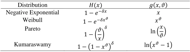
𝐻(𝑥) = 1 − 𝑒−𝛿𝑔(𝑥,𝜗) _{, 𝛿 > 0. (16)}

The distribution with form (16) is called general exponential form distribution, see Mokhlis et al. (2017). Many distributions have cumulative distribution functions satisfying the form in (16). Table 1 presents some examples of these distributions.

Table 1: The cumulative distribution function of some distributions that belongs to the general exponential form

Distribution 𝐻(𝑥) 𝑔(𝑥, 𝜗)

Negative Exponential 1 − 𝑒−𝛿𝑥 𝑥

Weibull _{1 − 𝑒}−𝛿𝑥𝜗 _𝑥𝜗

Pareto

1 − (𝜗 𝑥)

𝛿

ln (𝑥 𝜗)

Kumaraswamy _{1 − (1 − 𝑥}𝜗₎𝛿 ln(𝑥𝜗− 1)

Assume that the cumulative distribution functions of the stresses 𝑋₁ and 𝑋₂, and strength

𝑌 are given by

𝐺_𝑖(𝑥) = 1 − 𝑒−𝜆𝑖𝑔(𝑥,𝜗) ; 𝜆_𝑖 > 0, 𝑖 = 1, 2_{, and}

𝐹(𝑥) = 1 − 𝑒−𝛿𝑔(𝑥,𝜗) _{, 𝛿 > 0.}

(17) (18)

By substituting the forms of 𝐺𝑖(𝑥), 𝑖 = 1,2 and 𝐹(𝑥) given by (17) and (18) respectively,

𝐼_𝑎,𝑏𝑖 _{= ∫[1 − 𝑒}−𝛿𝑔(𝑥,𝜗)_]𝑎_[𝑒−𝛿𝑔(𝑥,𝜗)_]𝑏 _{d(1 − 𝑒}−𝜆_𝑖𝑔(𝑥,𝜗)₎ ∞

0

= ∑ (𝑎

𝑙) (−1)𝑙

𝜆_𝑖 (𝑙 + 𝑏)𝛿 + 𝜆_𝑖

𝑎

𝑙=0

= 𝐼_𝑎,𝑏𝑖 _{(𝛿, 𝜆}

𝑖) , 𝑖 = 1,2, (19)

which does not contain the parameter 𝜗. Substituting (19) in (12), (14), and (15), we obtain exact stress-strength reliability formulas for R_(𝑠:𝑠)(𝑘, 𝑛, 𝑐), R_{(𝑠:𝑠)𝑢}(𝑘, 𝑛, 𝑐), and

R(𝑠:𝑠)𝑏(𝑘, 𝑛, 𝑐). Since (19) does not contain the parameter 𝜗, the stress-strength reliability

formulas also do not contain the parameter 𝜗.

Case II

Suppose that the distributions of stresses 𝑋₁ and 𝑋₂ are negative exponential, with cumulative distribution functions are given by

𝐺𝑖(𝑥) = 1 − 𝑒−𝜆𝑖𝑥, 𝑖 = 1,2. (20)

Let the distribution of the strength 𝑌 is a generalized Lindley distribution, with probability distribution and cumulative distribution function given respectively by

𝑓(𝑦) = 1 1 + 𝜃[

𝜃𝛼+1_𝑦𝛼−1

𝛤(𝛼) +

𝜃𝛽_𝑦𝛽−1

𝛤(𝛽) ] 𝑒−𝜃𝑦, and

𝐹(𝑥) = 𝑝(𝑌 ≤ 𝑥) = 1 1 + 𝜃[

𝜃𝛾(𝛼, 𝜃𝑥) 𝛤(𝛼) +

𝛾(𝛽, 𝜃𝑥)

𝛤(𝛽) ] , 𝜃, 𝛼, 𝛽 > 0,

(21)

where 𝛾(𝑠, 𝑣𝑥) is a lower incomplete gamma. We can easily see that 𝑓(𝑦) is a mixture of two gamma distributions, with parameters (𝜃, 𝛼) and (𝜃, 𝛽) with probabilities _1+𝜃𝜃 and

1

1+𝜃 respectively. Substituting 𝐺𝑖(𝑥), i = 1,2 and 𝐹(𝑥) given by (20) and (21)

respectively in (13), we have

𝐼_𝑎,𝑏𝑖 = ∫ [∞ _1+𝜃1 [𝜃𝛾(𝛼,𝜃𝑥)_𝛤(𝛼) +𝛾(𝛽,𝜃𝑥)_𝛤(𝛽) ] ]𝑎[1 −_1+𝜃1 [𝜃𝛾(𝛼,𝜃𝑥)_𝛤(𝛼) +𝛾(𝛽,𝜃𝑥)_𝛤(𝛽) ] ]𝑏d(1 − 𝑒−𝜆𝑖𝑥)

0 ₍₂₂₎

= 𝐼_𝑎,𝑏𝑖 _{(𝜃, 𝛼, 𝛽, 𝜆}

𝑖), 𝑖 = 1,2.

The above integral can be obtained numerically, and hence the expression for

R_(𝑠:𝑠)(𝑘, 𝑛, 𝑐),R_{(𝑠:𝑠)𝑢}(𝑘, 𝑛, 𝑐), and R_{(𝑠:𝑠)𝑏}(𝑘, 𝑛, 𝑐).

Estimation of The Stress-Strength Reliability

Case I

As an application of the general exponential form, we take for simplicity 𝑔(𝑥, 𝜗) = 𝑥. The maximum likelihood estimator of R_(𝑠:𝑠)(𝑘, 𝑛, 𝑐), R_{(𝑠:𝑠)𝑢}(𝑘, 𝑛, 𝑐), and R_{(𝑠:𝑠)𝑏}(𝑘, 𝑛, 𝑐), can be obtained by replacing the parameters in (19) by their corresponding maximum likelihood estimators. For obtaining the maximum likelihood estimator of the parameters, let 𝑋1, 𝑋2, … , 𝑋𝑛_𝑖; 𝑖 = 1,2, and 𝑌1, 𝑌2, … , 𝑌𝑛3be samples of size 𝑛𝑖, 𝑖 = 1,2, and 𝑛3 from

𝜆̂_𝑖 = 𝑛𝑖 ∑𝑛𝑖 𝑋_𝑟

𝑟=0

, 𝑖 = 1,2, and

𝛿̂ = 𝑛3 ∑𝑛3 𝑌_𝑟

𝑟=0

.

(23)

(24)

Hence

𝐼̂_𝑎,𝑏𝑖 (𝛿̂, 𝜆̂𝑖) = ∑ (

𝑎

𝑙) (−1)𝑙

𝑛𝑖∑𝑛𝑟=03 𝑌𝑟

𝑛_𝑖∑𝑛3 𝑌_𝑟

𝑟=0 + (𝑙 + 𝑏)𝑛3∑𝑛𝑟=0𝑖 𝑋𝑟 𝑎

𝑙=0

, 𝑖 = 1,2. (25)

Replacing 𝐼_𝑎,𝑏𝑖 , 𝑖 = 1,2 in Equations (12), (14), and (15) by 𝐼̂_𝑎,𝑏𝑖 (𝛿̂, 𝜆̂_𝑖) given by (25), we get the maximum likelihood estimators R̂_(𝑠:𝑠)(𝑘, 𝑛, 𝑐), R̂_{(𝑠:𝑠)𝑢}(𝑘, 𝑛, 𝑐), and R̂_{(𝑠:𝑠)𝑏}(𝑘, 𝑛, 𝑐) of R_(𝑠:𝑠)(𝑘, 𝑛, 𝑐),R_{(𝑠:𝑠)𝑢}(𝑘, 𝑛, 𝑐), andR_{(𝑠:𝑠)𝑏}(𝑘, 𝑛, 𝑐), respectively.

Case II

The maximum likelihood estimators of the parameters 𝜆𝑖, 𝑖 = 1,2 are given by (23). Since

the generalized Lindley distribution in (21) is a mixture of two gamma distributions, we use the EM algorithm for obtaining the estimators 𝜃̂, 𝛼̂, and 𝛽̂ of 𝜃, 𝛼, and 𝛽 respectively. Estimators of R_(𝑠:𝑠)(𝑘, 𝑛, 𝑐), R_{(𝑠:𝑠)𝑢}(𝑘, 𝑛, 𝑐), and R_{(𝑠:𝑠)𝑏}(𝑘, 𝑛, 𝑐) are obtained by substituting the parameters with their corresponding estimators 𝜃̂, 𝛼̂, and 𝛽̂.

Numerical Illustration

Tables (2), (3), and (4) present the exact stress-strength reliabilities for case I (same general exponential form distributions), with 𝑔(𝑥, 𝜗) = 𝑥, while Tables (5), (6), and (7) illustrate the reliabilities for case II (different forms of distributions), showing the effect of position of the change point 𝑐, the value of 𝑘 with respect to 𝑛, and different parameters, on reliabilities. Using R-programming we compute R_(𝑠:𝑠)(𝑘, 𝑛, 𝑐),

R(𝑠:𝑠)𝑢(𝑘, 𝑛, 𝑐), and R(𝑠:𝑠)𝑏(𝑘, 𝑛, 𝑐) with 𝑛 = 6, 𝑘 = (2, 3, 𝑎𝑛𝑑 4) , and different values

of the parameters of the distributions of the stresses and strength, with different values of

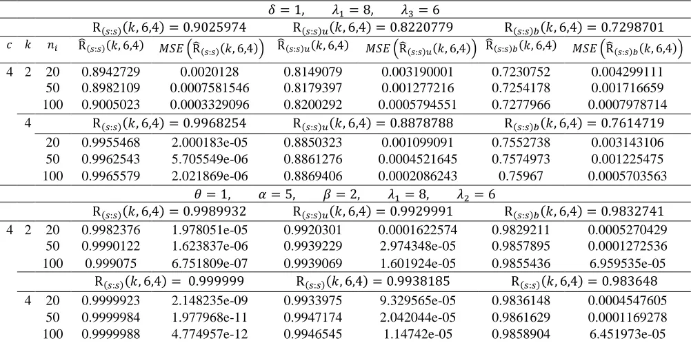
𝑐 = (2, 𝑎𝑛𝑑 4)𝑖. 𝑒(𝑐 ≤ 𝑘 , 𝑎𝑛𝑑 𝑐 > 𝑘). In Table (8) we present the maximum likelihood estimator of the reliabilities, obtained in Section 5. The estimators R̂_(𝑠:𝑠)(𝑘, 𝑛, 𝑐),

R̂_{(𝑠:𝑠)𝑢}(𝑘, 𝑛, 𝑐), and R̂_{(𝑠:𝑠)𝑏}(𝑘, 𝑛, 𝑐), that appear in these table are the average of 1000 repetitions, and we take 𝑛𝑖 = 20, 50, 100 , 𝑖 = 1,2,3. The mean square error of the

estimators is also calculated to indicate the accuracy of the estimators.

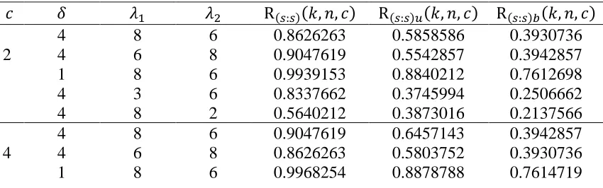
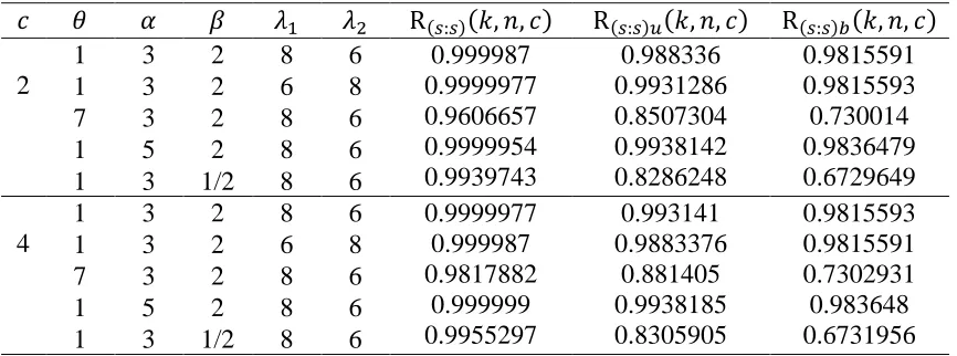
It is clear from Tables (2) to (7) that all reliabilities increase as 𝑘 increases for all cases of

𝑐, and for the different values of the parameters. The position of change point 𝑐 also influence the reliability according to the rate of stress before or after this point and number of components under this stress. We also see the effect of the strength and stresses parameters, on the reliability of the system in both cases I, and II. For case I, for the strength parameters, we can see that the increase of 𝛿 causes decrease in the reliability, while for stresses parameters, as 𝜆₁ or 𝜆₂ increase the reliability increases. From Tables (2 − 4), we see that the highest value of the reliability is attained for the largest values of 𝜆1 and 𝜆2, and the smallest value of 𝛿. Also, for generalized Lindley

strength, we see from Tables (5 − 7) as 𝜃 increases the reliability decreases, but as

attained when the values of 𝛼, 𝛽, and 𝜆_𝑖(𝑖 = 1,2) are large and 𝜃 is small. From Table (8), we see that bias and the mean square errors are small. The mean square error in all cases decreases by increasing the sample size. However, the estimators are satisfactory. Also, we see that 𝑀𝑆𝐸 (R̂_(𝑠:𝑠)(𝑘, 𝑛, 𝑐)) < 𝑀𝑆𝐸 (R̂_{(𝑠:𝑠)𝑢}(𝑘, 𝑛, 𝑐)) <

𝑀𝑆𝐸 (R̂_{(𝑠:𝑠)𝑏}(𝑘, 𝑛, 𝑐)) for all cases.

Table 2: Exact reliabilities for case I, with 𝒌 = 𝟐

𝑐 𝛿 𝜆₁ 𝜆₂ R_(𝑠:𝑠)(𝑘, 𝑛, 𝑐) R_{(𝑠:𝑠)𝑢}(𝑘, 𝑛, 𝑐) R_{(𝑠:𝑠)𝑏}(𝑘, 𝑛, 𝑐)

2

4 8 6 0.494228

0.5171429 0.8874074 0.3415416 0.2481481 0.3910534 0.3971429 0.8059259 0.2450666 0.1957672 0.3102453 0.3228571 0.7185185 0.1948052 0.1449735

4 6 8

1 8 6

4 3 6

4 8 2

4

4 8 6 0.5171429

0.494228 0.9025974 0.3048804 0.3088889 0.42 0.3917749 0.8220779 0.2304033 0.2511111 0.3228571 0.3102453 0.7298701 0.176432 0.1755556

4 6 8

1 8 6

4 3 6

4 8 2

Table 3: Exact reliabilities for case I, with 𝒌 = 𝟑

𝑐 𝛿 𝜆₁ 𝜆₂ R_(𝑠:𝑠)(𝑘, 𝑛, 𝑐) R_{(𝑠:𝑠)𝑢}(𝑘, 𝑛, 𝑐) R_{(𝑠:𝑠)𝑏}(𝑘, 𝑛, 𝑐)

2

4 8 6 0.7520924

0.8019048 0.9759259 0.6912801 0.4444444 0.5246753 0.5085714 0.8698413 0.3335807 0.3153439 0.3665224 0.3742857 0.7540741 0.2339349 0.184127

4 6 8

1 8 6

4 3 6

4 8 2

4

4 8 6 0.8019048

0.7520924 0.9844156 0.5461693 0.7333333 0.5971429 0.5310245 0.8805195 0.3472044 0.5577778 0.3742857 0.3665224 0.7571429 0.2203964 0.2066667

4 6 8

1 8 6

4 3 6

4 8 2

Table 4: Exact reliabilities for case I, with 𝒌 = 𝟒

𝑐 𝛿 𝜆1 𝜆2 R(𝑠:𝑠)(𝑘, 𝑛, 𝑐) R(𝑠:𝑠)𝑢(𝑘, 𝑛, 𝑐) R(𝑠:𝑠)𝑏(𝑘, 𝑛, 𝑐)

2

4 8 6 0.8626263

0.9047619 0.9939153 0.8337662 0.5640212 0.5858586 0.5542857 0.8840212 0.3745994 0.3873016 0.3930736 0.3942857 0.7612698 0.2506662 0.2137566

4 6 8

1 8 6

4 3 6

4 8 2

4

4 8 6 0.9047619

0.8626263 0.9968254 0.6457143 0.5803752 0.8878788 0.3942857 0.3930736 0.7614719

4 6 8

4 3 6 0.6800312 0.8755556 0.4005742 0.6266667 0.2481437 0.2177778

4 8 2

Table 5: Exact reliabilities for case II, with 𝒌 = 𝟐

𝑐 𝜃 𝛼 𝛽 𝜆₁ 𝜆₂ R_(𝑠:𝑠)(𝑘, 𝑛, 𝑐) R_{(𝑠:𝑠)𝑢}(𝑘, 𝑛, 𝑐) R_{(𝑠:𝑠)𝑏}(𝑘, 𝑛, 𝑐)

2

1 3 2 8 6 0.9978886

0.9986011 0.8136749 0.9985046 0.8411834 0.9875958 0.9912793 0.7518598 0.992505 0.7229847 0.9804053 0.9810692 0.6855084 0.9828109 0.6116767

1 3 2 6 8

7 3 2 8 6

1 5 2 8 6

1 3 1/2 8 6

4

1 3 2 8 6 0.9986011

0.9978886 0.8347424 0.9989932 0.8535313 0.9920017 0.9869422 0.7774817 0.9929991 0.7354143 0.9810692 0.9804053 0.6998564 0.9832741 0.6207246

1 3 2 6 8

7 3 2 8 6

1 5 2 8 6

1 3 1/2 8 6

Table 6: Exact reliabilities for case II, with 𝒌 = 𝟑

𝑐 𝜃 𝛼 𝛽 𝜆₁ 𝜆₂ R_(𝑠:𝑠)(𝑘, 𝑛, 𝑐) R_{(𝑠:𝑠)𝑢}(𝑘, 𝑛, 𝑐) R_{(𝑠:𝑠)𝑏}(𝑘, 𝑛, 𝑐)

2

1 3 2 8 6 0.9998605

0.9999604 0.9266386 0.9999275 0.9692297 0.9883034 0.9930054 0.8234927 0.9937484 0.8114427 0.9814962 0.981542 0.716885 0.9836141 0.6638775

1 3 2 6 8

7 3 2 8 6

1 5 2 8 6

1 3 1/2 8 6

4

1 3 2 8 6 0.9999604

0.9998605 0.9582906 0.9999771 0.9748258 0.9931194 0.9882719 0.8689741 0.9938056 0.8179912 0.981542 0.9814962 0.7228816 0.9836378 0.666214

1 3 2 6 8

7 3 2 8 6

1 5 2 8 6

1 3 1/2 8 6

Table 7: Exact reliabilities for case II, with 𝒌 = 𝟒

𝑐 𝜃 𝛼 𝛽 𝜆1 𝜆2 R(𝑠:𝑠)(𝑘, 𝑛, 𝑐) R(𝑠:𝑠)𝑢(𝑘, 𝑛, 𝑐) R(𝑠:𝑠)𝑏(𝑘, 𝑛, 𝑐)

2

1 3 2 8 6 0.999987

0.9999977 0.9606657 0.9999954 0.9939743 0.988336 0.9931286 0.8507304 0.9938142 0.8286248 0.9815591 0.9815593 0.730014 0.9836479 0.6729649

1 3 2 6 8

7 3 2 8 6

1 5 2 8 6

1 3 1/2 8 6

4

1 3 2 8 6 0.9999977

0.999987 0.9817882 0.999999 0.9955297 0.993141 0.9883376 0.881405 0.9938185 0.8305905 0.9815593 0.9815591 0.7302931 0.983648 0.6731956

1 3 2 6 8

7 3 2 8 6

1 5 2 8 6

Table 8: Estimated reliabilities

𝛿 = 1, 𝜆1= 8, 𝜆3= 6

R(𝑠:𝑠)(𝑘, 6,4) = 0.9025974 R(𝑠:𝑠)𝑢(𝑘, 6,4) = 0.8220779 R(𝑠:𝑠)𝑏(𝑘, 6,4) = 0.7298701 𝑐 𝑘 𝑛𝑖 R̂(𝑠:𝑠)(𝑘, 6,4) 𝑀𝑆𝐸 (R̂(𝑠:𝑠)(𝑘, 6,4)) R̂(𝑠:𝑠)𝑢(𝑘, 6,4) 𝑀𝑆𝐸 (R̂(𝑠:𝑠)𝑢(𝑘, 6,4)) R̂(𝑠:𝑠)𝑏(𝑘, 6,4) 𝑀𝑆𝐸 (R̂(𝑠:𝑠)𝑏(𝑘, 6,4))

4 2 20 0.8942729 0.0020128 0.8149079 0.003190001 0.7230752 0.004299111 50 0.8982109 0.0007581546 0.8179397 0.001277216 0.7254178 0.001716659 100 0.9005023 0.0003329096 0.8200292 0.0005794551 0.7277966 0.0007978714

4 R_(𝑠:𝑠)(𝑘, 6,4) = 0.9968254 R_{(𝑠:𝑠)𝑢}(𝑘, 6,4) = 0.8878788 R_{(𝑠:𝑠)𝑏}(𝑘, 6,4) = 0.7614719

20 0.9955468 2.000183e-05 0.8850323 0.001099091 0.7552738 0.003143106 50 0.9962543 5.705549e-06 0.8861276 0.0004521645 0.7574973 0.001225475 100 0.9965579 2.021869e-06 0.8869406 0.0002086243 0.75967 0.0005703563

𝜃 = 1, 𝛼 = 5, 𝛽 = 2, 𝜆1= 8, 𝜆2= 6

R(𝑠:𝑠)(𝑘, 6,4) = 0.9989932 R(𝑠:𝑠)𝑢(𝑘, 6,4) = 0.9929991 R(𝑠:𝑠)𝑏(𝑘, 6,4) = 0.9832741

4 2 20 0.9982376 1.978051e-05 0.9920301 0.0001622574 0.9829211 0.0005270429 50 0.9990122 1.623837e-06 0.9939229 2.974348e-05 0.9857895 0.0001272536 100 0.999075 6.751809e-07 0.9939069 1.601924e-05 0.9855436 6.959535e-05

R(𝑠:𝑠)(𝑘, 6,4) = 0.999999 R(𝑠:𝑠)(𝑘, 6,4) = 0.9938185 R(𝑠:𝑠)(𝑘, 6,4) = 0.983648

4 20 0.9999923 2.148235e-09 0.9933975 9.329565e-05 0.9836148 0.0004547605 50 0.9999984 1.977968e-11 0.9947174 2.042044e-05 0.9861629 0.0001169278 100 0.9999988 4.774957e-12 0.9946545 1.14742e-05 0.9858904 6.451973e-05

Conclusions

In this paper explicit expressions for R(𝑘, 𝑛, 𝑐; P), R𝑢(𝑘, 𝑛, 𝑐; P), and R𝑏(𝑘, 𝑛, 𝑐; P) are

obtained conditioning on the state of the change point at position 𝑐 (working or failed). Then consequently, R_(𝑠:𝑠)(𝑘, 𝑛, 𝑐), R_{(𝑠:𝑠)𝑢}(𝑘, 𝑛, 𝑐), and R_{(𝑠:𝑠)𝑏}(𝑘, 𝑛, 𝑐) are presented when the change in the components reliabilities is due to change in the stress. This means that the components from 1 to 𝑐 are subjected to a common stress, 𝑋1, while the components

from 𝑐 + 1 to 𝑛 are subjected to a different common stress, 𝑋2. The strengths of all

components 1 to 𝑛 are independent and identical. The stress-strength reliabilities of linear consecutive k-out-of-n: F system, unipolar-relayed and bipolar-relayed linear consecutive k-out-of-n: F systems are obtained for any distribution of stresses 𝑋_𝑖, 𝑖 = 1,2, and strength 𝑌. As application, two cases are discussed: Case I and Case II. In Case I, the stresses and strength are assumed to have the same form of distributions (as an example, general exponential form, in (16)). Exact formulas are obtained in this case, showing that the forms of the stress-strength reliabilities for all systems do not involve the parameter

𝜗. In Case II, the stresses and strength are assumed to have different forms of distributions (as an example, negative exponential distribution for stresses and generalized Lindley distribution for strength). Numerical illustrations are applied through simulation studies for both cases, to detect the effect of position of the change point 𝑐, the value of 𝑘 with respect to 𝑛, and different distributions parameters, on the stress strength reliabilities. For both Cases I and II, the simulation studies showed that R_(𝑠:𝑠)(𝑘, 𝑛, 𝑐),

number of components under that stress. Also, the stress-strength reliability of all systems is sensitive to the distributions parameters involved in its form. The maximum likelihood estimators R̂_(𝑠:𝑠)(𝑘, 𝑛, 𝑐), R̂_{(𝑠:𝑠)𝑢}(𝑘, 𝑛, 𝑐) and R̂_{(𝑠:𝑠)𝑏}(𝑘, 𝑛, 𝑐) of R_(𝑠:𝑠)(𝑘, 𝑛, 𝑐),

R_{(𝑠:𝑠)𝑢}(𝑘, 𝑛, 𝑐) and R_{(𝑠:𝑠)𝑏}(𝑘, 𝑛, 𝑐), are their mean square errors are also calculated to indicate the accuracy of the estimation.

References

1. Akici, F. (2010). Reliability Analysis of Consecutive-k Systems in a Stress-Strength Setup. (Master’s thesis, Graduate School of Natural and Applied Sciences).

2. Al-Hussaini, E. K. (1999). Predicting observables from a general class of distributions. Journal of Statistical Planning and Inference, 79, 79-91.

3. Birnbaum, Z. (1956). On a use of the Mann-Whitney statistic. Proceedings of the third Berkeley symposium on mathematical statistics and probability. University of California Press Berkeley, 13-17.

4. Birnbaum, Z. and Mccarty, R. (1958). A Distribution-Free Upper Confidence Bound for P{Y<X}, Based on Independent Samples of X and Y. The Annals of Mathematical Statistics, 558-562.

5. Chao, M., Fu, J. and Koutras, M. (1995). Survey of reliability studies of consecutive-k-out-of-n: F and related systems. IEEE Transactions on Reliability, 44, 120-127.

6. Chiang, D. T. and Niu, S. C. (1981). Reliability of consecutive-k-out-of-n: F system. IEEE Transactions on Reliability, 30, 87-89.

7. Derman, C., Lieberman, G. J. and Ross, M. S. (1982). On the consecutive-k-of-n: F system. IEEE Transactions on Reliability, 31, 57-63.

8. Elbatal, I., Merovci, F. and Elgarhy, M. (2013). A new generalized Lindley distribution. Mathematical theory and Modeling.

9. Eryılmaz, S. (2008). Consecutive k-out-of-n: G system in stress-strength setup. Communications in Statistics Simulation and Computation, 37, 579-589.

10. Ge, G. and Wang, L. (1990). Exact reliability formula for consecutive-k-out-of-n: F systems with homogeneous Markov dependence. IEEE Transactions on Reliability, 39, 600-602.

11. Gökdere, G., Gürcan, M. and Kılıç, M. B. (2016). A new method for computing the reliability of consecutive k-out-of-n: F systems. Open Physics, 14, 166-170. 12. Hwang, F. (1982). Fast solutions for consecutive-k-out-of-n: F system. IEEE

Transactions on Reliability, 31, 447-448.

13. Hwang, F. (1988). Relayed consecutive-k-out-of-n: F lines. IEEE Transactions on Reliability, 37, 512-514.

15. Jung, K. H. and Kim, H. (1993). Linear consecutive-k-out-of-n: F system reliability with common-mode forced outages. Reliability Engineering & System Safety, 41, 49-55.

16. Kossow, A. and Preuss, W. (1989). Reliability of consecutive-k-out-of-n: F systems with nonidentical component reliabilities. IEEE Transactions on Reliability, 38, 229-233.

17. Lambiris, M. and Papastavridis, S. (1985). Exact reliability formulas for linear & circular consecutive-k-out-of-n: F systems. IEEE Transactions on Reliability, 34, 124-126.

18. Mokhlis, N. A. (2001). consecutive k-out-of-n systems. In Advances, in Reliability, (N.Balakrishnan & C.R.Rao, eds.). Elsevier, New York, 237-280". 19. Mokhlis, N. A., Ibrahim, E. J and Gharieb, D. M. (2017). Stress-strength

reliability with general form distributions. Communications in Statistics-Theory and Methods, 46, 1230-1246.