The Kumaraswamy Weibull Geometric Distribution with Applications

The Kumaraswamy Weibull Geometric Distribution with Applications

Mahdi Rasekhi

Department of Statistics, Malayer University, Malayer, Iran rasekhimahdi@gmail.com

Morad Alizadeh

Department of Statistics ,Persian Gulf University, Bushehr, Iran moradalizadeh78@gmail.com

G.G. Hamedani

Department of Mathematics, Statistics and Computer Science Marquette University, Milwaukee, USA

g.hamedani@mu.edu

Abstract

In this work, we study the kumaraswamy weibull geometric (Kw-WG) distribution which includes as special cases, several models such as the kumaraswamy weibull distribution, kumaraswamy exponential distribution, weibull geometric distribution, exponential geometric distribution, to name a few. This distribution was monotone and non-monotone hazard rate functions, which are useful in lifetime data analysis and reliability. We derive some basic properties of the Kw-WG distribution including non-central rth-moments, skewness, kurtosis, generating functions, mean deviations, mean residual life, entropy, order statistics and certain characterizations of our distribution. The method of maximum likelihood is used for estimating the model parameters and a simulation study to investigate the behavior of this estimation is presented. Finally, an application of the new distribution and its comparison with recent flexible generalization of weibull distribution is illustrated via two real data sets.

Keywords: Weibull Geometric distribution; Data Analysis; Moments; Entropy; Characterizations.

Introduction

Barreto-Souza et al. (2011) introduced a new extension of Weibull distribution (Weibull Geometric distribution) by compounding Weibull and Geometric distributions with probability density function (pdf) and cumulative distribution function (cdf)

and

respectively, where and .

On the other hand, Cordeiro and de Castro (2011) introduced the Kumaraswamy-G (Kw-G) class of distributions with the following pdf and cdf

where G(x) is a cdf with its corresponding pdf, g(x). Clearly, for a=b=1, we obtain the main distribution. The parameters a and b control the skewness and tail weights. The form of this class of distributions is simpler than the Beta-G class (Eugene et al., 2002) because it does not involve incomplete beta function. Nadarajah et al. (2012) obtained general results about this class of distributions.

In this paper, a more flexible five parameter generalization of Weibull distribution based on Kumaraswamy-G class and Weibull Geometric distribution, called Kumaraswamy Weibull Geometric (Kw−WG), is introduced. A comprehensive description of some of its mathematical properties is presented. The pdf of this model includes decreasing, right and left skew uni-bimodal shape and the hf of this distribution contain increasing, decreasing, unimodal, bathtube and non-monotone shape. The Kw-WG distribution includes some well-known class of distribution as special cases such as Kw-W, Kw-Rayleigh (Gomez et al, 2014), EW, Exponential Geometric (Adamidis and Loukas, 1998), Weibull Geometric (Barreto-Souza et al., 2011) to name a few.

This article is organized as follows. In Section 2, the new distribution with its pdf is proposed. Further, the distributional properties of the new distribution, such as the cdf, survival and hazard rate functions, moment generating function, non-central and descending factorial moments, mean deviation, Bonferroni and Lorenz curves, mean residual life and mean inactivity time, Renyi and q entropy functions and order statistics with its moments are discussed. Section 3 deals with the characterizations of this model based on truncated moments, hazard function, reversed hazard function and certain function of the random variable. In Section 4, the maximum likelihood estimation of the parameters and the Fisher information matrix are discussed and a simulation study to investigate behavior of the estimators is done. Applications of the proposed model are illustrated in Section 5. Concluding remarks are given in Section 6.

1 ( ) ( ) 2

( )

(1

)

(1

) ,

X

g

x

= −

p c



x

e

−

pe

( ) ( )

1

( )

,

1

e

G

x

pe

−

=

−

(

)

(

)

( ) ( ) ( ) 1 ( ) ,

( ) 1 1 ( ) ,

b a a X b a X

f x abg x G x G x

F x G x

− −

= −

= − −

(0, ), ,

The Kumaraswamy-Weibull Geometric distribution

The cdf of is defined by

(1)

where and are parameters. Its pdf has the form

(2)

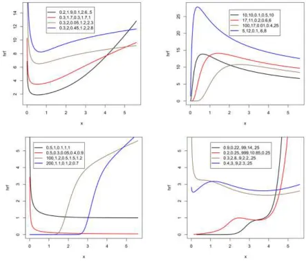
Note that, is a scale parameter and the other positive parameters a,b,p and c are shape parameters. The graphs of pdf in (2), for selected parameters values are given in Figure 1. This distribution is more flexible than Weibull Geometric distribution and can be model decreasing, right and left skew unimodal and bimodal data sets.

Figure 1: Plots of the pdf for some parameter values.

If X is a random variable with pdf (2), we write X~ . The survival and hazard rate functions corresponding to (2) are

and

(3)

( )

( )

1

( ) 1 ,

1 c c b a x X _x e S x pe   − −  _{ − }    = − _ _  _ − _   

, , , 0

a b c



1 ( ) 1 ( ) ( ) 2

( )

1 ( )

( )

1

( ) (1 ) (1 )

1

1

1 , 0.

1 c c c c c c a x

c c x x

X _x b a x x e

f x abc p c x e pe

pe e x pe      







1 ( ) 1 ( ) ( ) 2

( )

( )

( )

1

(1 ) (1 )

1 ( ) , 1 1 1 c c c c c c a x

c c x x

x

F a

x x

e

abc p c x e pe

pe h x e pe      





( )

( )

1

( ) 1 1 , 0,

1 c c b a x X _x e

F x x

respectively. The hf (3) is quite flexible for modeling survival data. See the plots of for selected parameter values given in Figure 2. The hf (3) can be increasing, decreasing, unimodal, bathtub and non monotone as shown in the Figure 2.

Figure 2: Plots of the Kw − WG(a,b,p,c,λ) hazard rate function for some parameter values.

Some properties of the Kw − WG distribution are:

A physical interpretation of the Kw − WG distribution (for positive integer value of a and b) is as follows. Suppose a system is made of b independent components and each component is made up of a independent subcomponents. Suppose the system fails if any of the b components fails and each component fails if all of the a subcomponents fail.

Let denote the lifetimes of the subcomponents within the jth component, j=1,…,b and let X denote the time to failure distribution of the entire system. The cdf of

( )

F h x

1

,...,

j ja

or

Therefore, X has the Kw − WG distribution given by (1).

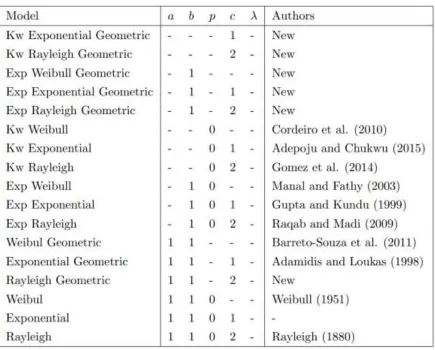
The distributions which are sub-models of the Kw − WG distribution are listed in Table 1.

Table 1: Some special cases of Kw − WG distribution

Asymptotics

The asymptotics of cdf, pdf and hf as x → 0 are given by

and





1 1

( ) 1 ( ,..., _b ) 1 1 ( ) b,

P X  x = −P X x X  x = − −P X x









(

) 1

1

(

,...,

)

1

1 ( (

))

.

Also, the asymptotics of cdf, pdf and hf as x → ∞ are given by

and

These equations show the effect of parameters on tails of distribution.

Extreme Value

If is a random sample from Kw−WG distribution and if

denotes the sample mean, then by usuall central limit theorem

approaches the standard normal distribution as n → ∞. One may be interested in the asymptotic of the extreme values and

For Kw − WG distribution, it can be seen that

and

Then it follows from Theorem 1.6.2 of Leadbetter et al. (1987) that there must be norming constant and such that

as n → ∞. Using Corollary 1.6.3 of Leadbetter et al. (1987), we can obtain the form of and .

Expansion for the density function

Let X follow the Kw− WG(a,b,p,c,λ) distribution. The pdf of X, using the generalized binomial expantions (Spiegel et al., 2009),

can be rewritten as the following series representation

(4)

0

(1 )n ( 1)i i, ,

i

n

z z n R

i 

=

 

− = _{ } −  

 



1

,

,...,

X X

X

1 2

( ... _n) /

X = X +X + +X n

( ( )) / ( )

n X−E X V x

1 2

( , ,..., )

n n

M =Max X X X mn =Min X X( 1, 2,...,Xn).

0, , 0

n n n

a  b c 

d

, ,

n n n

where

(5)

Moments and generating function

Some of the most important characteristics of a distribution can be studied through moments. For a random variable X having density function (2), is obtained by using Equation (4) and Gamma integral

as

(6)

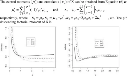
The skewness and kurtosis measures can be calculated from the ordinary moments using well−known relationships. Graphical representation of these quantities for some choices of parameter b as function of a, by fixing and , are given in Figures 3.

The central moments ( ) and cumulants ( ) of X can be obtained from Equation (6) as

and

respectively, where , etc. The pth descending factorial moment of X is

Figure 3: Skewness and kurtosis of the Kw − WG distribution as functions of a for some values of b.

(

)

E X

a

u

e

du

b

( )



=













p= c=



= 

r







1 0

( 1)

r

s s

r r s

s r s



 



r r s r s

s r s





 



1 1

,

,

3

2

where is the Stirling number of the first kind. Thus the factorial moments of X are given by

The moment genrating function (mgf) of X, can be expressed as

Thus the mgf of is

Quantile function

The quantile function, say , of the Kw WG distribution obtaines by inverting Equation (1) as

(7)

We can simulate data from the distribution by

where u has the uniform U(0,1) distribution.

Mean deviations

The amount of scatter in X is evidently measured to some extent by the totality of deviations from the mean and median. If X has the Kw− WG distribution (1), we can derive the mean deviations about the mean and about the median M as

and

respectively. The median M is obtained from Equation (7) as

These measures can be calculated from the relationships

and (8)

( )

(

)

X

M

t

=

E e

( , , , , ) Kw WG a b p c−



1

( ; , , , , )

( ; , , , , )

x

=

Q z a b p c



=

F

z a b p c



( , , , , ) Kw WG a b p c−



1

E X

( )

where is easily obtained from Equation (1) and From Equation (4) and using the incomplete gamma function we can obtain

(9)

Equation (9) is the basic value to compute the mean deviations and in Equation (8). It can also be used to determine Bonferroni and Lorenz curves. These curves have applications not only in economics in the study of income and poverty, but also in other fields like reliability, demography, insurance and medicine.

Mean residual life and mean inactivity time

The mean residual life has many applications in biomedical sciences, life insurance, maintenance and product quality control, economics and social studies, demography and product technology (see Lai and Xie, 2006). The MRL is given by

for t > 0, and it represents the expected additional life length for a unit, which is alive at age t.

The MRL of X can be computed as

where J(t) is Equation (9).

The mean inactivity time defined by (for t > 0) represents the waiting time elapsed since the failure of an item on condition that this failure had occurred in (0,t). The MIT of X is given by

where J(t) is Equation (9).

Entropy

The entropy of a random variable X is a measure of the uncertainty variation. The Renyi entropy is defined by

where and . Similarily, is expanded as follow

where

1

( )

F



0

( ) q _X( ) .

J q =



1 0

, z a u ,

a z u e du

_{( ) =} − −



1

d

d

( ) ( ),

X

m t =E X−t X t

*

( ) ( )

X

M t =E t−X X t

(10)

Therefore, the Renyi entropy for the Kw-WG distribution is given by

(11)

The q-entropy is defined by

Where ( and ), follows from (11) as

Order statistics and moments

In this section, we derive closed-form expressions for the pdf of the rth order statistic of X. Let be a random sample from the Kw − WG distribution with cdf and pdf given by (1) and (2), respectively. Let denote the order statistics obtained from this sample. The pdf of , say , is given by

where F(x) and f(x) are the cdf and pdf of X given by (1) and (2), respectively, and B(.,.) is the beta function. Similarily, expands as

where

The rth moment of the ith order statistic can be obtained from the following result: q

H

q  q  ( ) q

q X

J  f x dx −

=



q

J = −q e

1, 2,..., n

X X X

(1) (2)

...

X



X

 

X

( )i

X

i

X

f x

( )i ( )

X

f x

( )i

Characterizations

Characterizations of distributions is an important research area which has recently attracted the attention of many researchers. This section deals with various characterizations of Kw-WG family of distributions. These characterizations are based on: (i) a simple relationship between two truncated moments; (ii) the hazard function; (iii) the reverse hazard function; (iv) certain functions of the random variable. It should be mentioned that for characterization (i) the cdf need not have a closed form. We present our characterizations (i) − (iv) in four subsections.

Characterizations based on two truncated moments

In this subsection we present characterizations of Kw-WG distribution in terms of a simple rela-tionship between two truncated moments. This characterization result employs a theorem due to Gl¨anzel (1987) see Theorem 1 below. Note that the result holds also when the interval H is not closed. Moreover, as mentioned above, it could be also applied when the cdf F does not have a closed form. As shown in [10], this characterization is stable in the sense of weak convergence.

Theorem 1. Let (Ω, ℱ, 𝐏) be a given probability space and let 𝐻 = [𝑑, 𝑒] be an interval for some 𝑑 < 𝑒 (𝑑 = −∞, 𝑒 = ∞ might as well be allowed). Let 𝑋: Ω → 𝐻 be a continuous random variable with the distribution function 𝐹 and let 𝑔 and h be two real functions defined on 𝐻 such that

is defined with some real function . Assume that 𝑔, ℎ ∈ 𝐶1(𝐻), 𝜉 ∈ 𝐶2(𝐻) and 𝐹 is twice continuously differentiable and strictly monotone function on the set 𝐻. Finally, assume that the equation 𝜉ℎ = 𝑔 has no real solution in the interior of 𝐻. Then 𝐹 is uniquely determined by the functions 𝑔, ℎ and 𝜉 , particularly

where the function 𝑠 is a solution of the differential equation 𝑠′ = 𝜉

′_ℎ

𝜉ℎ−𝑔 and 𝐶 is the normalization constant, such that ∫_𝐻 𝑑𝐹 = 1.

Proposition 1. Let 𝑋: Ω → (0, ∞) be a continuous random variable and let

and



( ) 1

1 c c b a x x e h x pe   − − −  _{ − }    = −  _ _  −       ( ) ( )

1

( )

( )

1

e

g x

h x

for x > 0. The random variable X belongs to Kw-WG family (2) if and only if the function ξ defined in Theorem 1 has the form

Proof. Let X be a random variable with pdf (2), then

and

and finally

Conversely, if ξ is given as above, then

and hence

Now, in view of Theorem 1, X has density (2).

Corollary 1. Let 𝑋: Ω → (0, ∞) be a continuous random variable and let h(x) be as in Proposition 1.. The pdf of 𝑋 is (2) if and only if there exist functions 𝑔 and 𝜉 defined in Theorem 1 satisfying the differential equation

The general solution of the differential equation in Corollary 1 is

where D is a constant. Note that a set of functions satisfying the above differential

equation is given in Proposition 1 with . However, it should be also noted that

there are other triplets (h,g,ξ) satisfying the conditions of Theorem 1.

Characterization based on hazard function

It is known that the hazard function, , of a twice differentiable distribution function, F, satisfies the first order differential equation

(12)

For many univariate continuous distributions, this is the only characterization available in terms of the hazard function. The following characterization establish a non-trivial characterization of Kw-WG distribution, for a = 1, in terms of the hazard function, which is not of the trivial form given in (12).

Proposition 2. Let 𝑋: Ω → (0, ∞) be a continuous random variable. For a = 1,the pdf of X is (2) if and only if its hazard function satisfies the differential equation

(13)

with the initial condition for c > 1.

Proof. If X has pdf (2), then clearly (13) holds. Now, if (13) holds, then

or

which is the hazard function of the Kw-WG distribution for a = 1.

Characterization in terms of the reverse (or reversed) hazard function

The reverse hazard function, of a twice differentiable distribution function, F, is defined as

Proposition 3. Let 𝑋: Ω → (0, ∞) be a continuous random variable. For b = 1, the pdf of X is (2) if and only if its reverse hazard function satisfies the differential equation

(14)

Proof. If X has pdf (2), then clearly (14) holds. Now, if (14) holds, then

or

which is the reverse hazard function of the Kw-WG distribution. F

h

F

h

(0)

0

F

h

=

,

F

r

( )

F

Characterization based on certain functions of the random variable

The following propositions have already appeared in (Hamedani, 2013) , so we will just state them here which can be used to characterize Kw-WG distribution.

Proposition 4. Let 𝑋: Ω → (d, e) be a continuous random variable with cdf F. Let ψ(x) be a differentiable function on (d,e) with . Then for ,

If and only if

Proposition 5. Let 𝑋: Ω → (d, e) be a continuous random variable and let ψ(x) be a differentiable function on (d,e) with . Then for ,

implies

Remarks 3.4.1. (a) It is easy to see that for certain functions, e.g.,

and (d,e) = (0,∞) , Proposition 4 provides a characterization of Kw-WG

distribution.(b) Taking, e.g., and (d,e) = (0,∞) ,

Proposition 5 provides a characterization of Kw-WG distribution for b = 1. (c) Clearly

there are other suitable functions ψ, we choose the above ones for simplicity.

Maximum likelihood estimation

We calculate the maximum-likelihood estimates (MLEs) of the parameters of the Kw-WG dis-tribution from complete samples only. Let Let be a random sample of size n from the Kw − WG(a,b,p,c,λ) distribution. The log-likelihood function for the vector of parameters can be written as

(15)

The log-likelihood can be maximized either directly by using the R program or by solving the nonlinear likelihood equations obtained by differentiating Equation (15).





lim ( ) 1

x d

x



+

→ =

lim ( ) 1

x e x







( ) 1 ,

1 c c a x x e x pe    = − _ − −₋ _ −   1 b b



1

( )

,

1

1

e

b

x

b

pe



=







−









=

+

−





1

,

,...,

x x

x

( , , , , )

a b p c



=

Simulation

In this section, we investigate the behavior of the ML estimators for a finite sample size (n). Simulation study based on Kw−WG(a,b,p,c,λ) distribution is carried out. The random variables are generated by using quantile technique presented in section 2.5 from Kw − WG(a,b,p,c,λ). A simulation study consisting of following steps is being carried out for each (a,b,p,c,λ) such as (0.5,0.5,0.1,3,0.4) (unimodal pdf), (0.25,0.25,0.95,10.85,0.25) (bimodal pdf), (0.5,0.5,0.1,3,0.4), (0.9,1.6,0.9,2,0.5) (increasing pdf) for n = 200,400,600.

• Choose the initial value of for the corresponding elements of the parameter vector , to specify Kw − WG(a,b,p,c,λ) distribution

• choose sample size n

• generate 5000 independent samples of size n from Kw − WG(a,b,p,c,λ).

• compute the ML estimate of for each of the 5000 samples

• compute the mean of the obtained estimators over all 5000 samples, the average bias

and the average mean square error

of simulated estimates.

Table 2 presents bias and mean square error for some selected parameter values and for different values of n. The values in Table 2 indicate that the estimates are stable and are more close to the true values when the sample sizes increased.

Table 2: Average bias in paranthesis and average MSE of the simulated estimates 0

( ,

,

,

,

)

T

a b p c



=

θ

( , , , , )

a b p c



=

θ

ˆ

n

Application and comparison

In this section, we present an application of the Kw − WG distribution using two real data sets. The first data set is given by Raqab and Kundu (2009) on the gauge lengths of 20 mm and consists of n = 74 observations. Also, these data set is used by Nofal et al. (2015) and Afify et al. (2016). We use the same data to compare the Kw − WG model with some rival models. The second data set is an uncensored data set from Murthy et al. (2004) (page 180) consisting of 50 observation on failure times of 50 Components (per 1000 hours). These data were also analyzed by Merovci and Elbatal (2013).

In the applications, the information about the hazard shape can help in selecting a

particular model. For this aim, a device called the total time on test (TTT) plot (Aarset,

1987) is useful. The TTT plot is obtained by plotting

where r = 1,...,n and (i = 1,...,n) are the order statistics of the sample, against r/n. If

the shape is a straight diagonal the hazard is constant. It is convex shape for decreasing

hazards and concave shape for increasing hazards. The bathtub-shaped hazard is obtained

when the first convex and then concave and for bimodal shape hazard, the TTT plot is

first concave and then convex. The TTT plot for both datasets presented in Figure 4.

These figures indicates that first and second dataset has increasing hazard and decreasing

failure rate function.

Therefore, the proposed Kw-WG model can be used to fit these data, since it can be model data with increasing and decreasing shapes of failure rate functions. The MLE of parameters, maximized log-likelihood function, Cramer-von Mises ( ) and AndersonDarling ( ) statistics are determined for fitting distributions.

For first data, we compare the fits of the new model with models: Kumaraswamy complemen-tary Weibull Geometric (Kw-CWG) (Afify et al, 2016), Beta Weibull (BW) (Lee et al., 2007), McDonald Weibull (McW) (Cordeiro et al., 2014), modified Beta Weibull (MBW) (Khan, 2015), Kumaraswamy Weibull (Kw-W) (Cordeiro et al., 2010), complementary Weibull Geometric (CWG) (Tojeiro et al., 2014) and Weibull Geometric (WG) (Barreto-Souza et al., 2011) distributions. The rival models for second data set are McDonald Modified Weibull (McMW) (Merovci and El-batal, 2013), McDonald Weibull (McW) (Cordeiro et al., 2014), Beta Weibull (BW) (Lee et al., 2007), Weibull Geometric (WG) (Barreto-Souza et al., 2011) and Beta modified Weibull (BMW) (Silva et al., 2010) distributions.

Table 3 and Table 4 include the MLEs of the model parameters, their corresponding standard errors (SEs) and the values of maximized log-likelihood function, and . Figures 5 and 6 displays histogram and estimated cdf of dataset with fitted Kw-WG distribution.

( ) ( ) ( )

1 1

( / ) ( ) /

n n

i r i

i i

G r n y n r y y

= =

  

=_{ }+ − _

 







( )i

y

*

W

*

A

*

Figure 4: TTT-plot for the first dataset (left figure) and for the second dataset (right figure).

Table 3: MLEs, their SEs (in parentheses), maximized log-likelihood, , and for the fitted models to the first data set

*

W

*

Table 4: MLEs, their SEs (in parentheses), maximized log-likelihood, , and for the fitted models to the second data set

Figure 5: Left panel: The Kw − WG density estimate superimposed on the histogram of

gauge length data . Right panel: The Kw − WG cdf estimates and empirical cdf.

Figure 6: Left panel: The Kw − WG density estimate superimposed on the histogram of

failure times data . Right panel: The Kw − WG cdf estimates and empirical cdf.

*

W

*

It is seen that the proposed Kw−WG model provides the best fit for both data sets when considering maximized log likelihood, Anderson-Darling and Cramer-von Mises goodness of fit statistics.

Conclusion

This paper proposed a new five parameter lifetime distribution by using Kumaraswamy-G class of distributions and Weibull Kumaraswamy-Geometric distribution. It contains a number of known special submod-els such as Kumaraswamy Weibull distribution, Kumaraswamy Exponential distribution, Weibull Geometric distribution, Exponential Geometric distribution and etc. We have studied many statistical properties of Kw − WG distribution including its probability density function, explicit algebraic expressions of survival and hazard functions, mean deviation, order statistics and its mo-ments, entropy, moment generating function and its characterizations. The maximum likelihood estimation is discussed and a simulation study for its behavior is done. It is suitable for increasing, decreasing, bathtub shaped, and non monotone shaped hazard rates, indicating its flexibility for modeling lifetime data with various shaped hazard rate functions. Accordingly, we expect that the new distribution may attract wider applications in reliability, biology, and lifetime data analysis.

References

1. Adamidis, K., Loukas, S. (1998). A lifetime distribution with decreasing failure rate. Statistics and Probability Letters, 39: 35-42.

2. Adepoju, K.A., Chukwu, O.I. (2015). Maximum Likelihood Estimation of the Kumaraswamy Exponential Distribution with Applications. Journal of Modern Applied Statistical Methods, 14: 208-214.

3. Alizadeh, M., Rasekhi, M., Yousof, H.M. and Hamedani, G.G. (2017). The Transmuted Weibull-G Family of Distributions. Hacettepe Journal of Mathematics and Statistics. forthcoming.

4. Afify, A.Z., Cordeiro, G.M., Butt, N.S., Ortega, E.M.M. and Suzuki, A.K. (2016). A New Lifetime Model with Variable Shapes for the Hazard Rate. Brazilian Journal of Probability and Statistics, accepted and presented in future papers. 5. Aarset, M.V. (1987). How to identify bathtub hazard rate. IEEE Transection

Reliability, 36:106-108.

6. Barreto-Souza, W., Morais, A.L. and Cordeiro, G.M. (2011). The Weibull-geometric distribu-tion. Journal of Statistical Computation and Simulation, 60: 35-42.

7. Cordeiro, G.M. and de Castro, M. (2011). A new family of generalized distributions. Journal of Statistical Computation and Simulation, 81: 883-898. 8. Cordeiro, G.M., Hashimoto, E.M. and Ortega, E.M.M. (2014). The McDonald

Weibull model. Statistics: A Journal of Theoretical and Applied Statistics, 48: 256-278.

9. Cordeiro, G.M., Ortega, E.M.M. and Nadarajah, S. (2010). The Kumaraswamy Weibull distribution with application to failure data. Journal of the Franklin Institute, 347: 1317-1336.

11. Gl¨anzel, W. (1987). A characterization theorem based on truncated moments and its application to some distribution families. Mathematical Statistics and Probability Theory (Bad Tatz-mannsdorf, 1986), Vol.B, Reidel, Dordrecht: 75-84. 12. Gl¨anzel, W. (1990). Some consequences of a characterization theorem based on truncated moments. Statistics: A Journal of Theoretical and Applied Statistics, 21 (4): 613-618.

13. Gomes, A. E., da Silva, C.Q., Cordeiro, G.M. and Ortega, E.M.M. (2014). A new lifetime model: the Kumaraswamy generalized Rayleigh distribution. Journal of Statistical Computation and Simulation, 84: 290-309.

14. Gupta, R.D. and Madi, M.T. (1999). Generalized exponential distributions: Theory and methods. Australian and New Zealand Journal of Statistics, 41: 173-188.

15. Hamedani, G.G. (2013). On certain generalized gamma convolution distributions. II, Technical Report, No. 484, MSCS, Marquette University.

16. Khan, M.N. (2015). The modified beta Weibul distribution with applications. Hacettepe Journal of Mathematics and Statistics, 44: 1553-1568.

17. Lai, C.D., and Xie, M. (2006). Stochastic ageing and dependence for reliability. Springer Science and Business Media.

18. Lee, C., Famoye, F., and Olumolade, O. (2007). Beta-Weibull distribution: some properties and applications to censored data. Journal of Modern Applied Statistical Methods, 6: 173-186.

19. Leadbetter, M.R., Lindgren, G., and Rootzen, H. (1987). Extremes and related Properties of random sequences and processes. Springer, Verlag, New Yourk. 20. Manal, M.N. and Fathy, H.E. (2003). On the Exponentiated Weibull Distribution.

Communications in Statistics - Theory and Methods, 32: 1317-1336.

21. Merovci, F. and Elbatal I. (2013). The mcdonald modified weibull distribution: properties and application.arXiv preprint arXiv:1309.2961.

22. Murthy, D. P., Xie, M., and Jiang, R. (2004). Weibull models (Vol. 505). John Wiley and Sons.

23. Nadarajah, S.,Cordeiro, G.M. and Ortega, E.M.M. (2012).General results for the Kumaraswamy-G distribution. Journal of Statistical Computation and Simulation, 82: 951-979.

24. Nofal, Z. M., Afify, A. Z., Yousof, H. M. and Cordeiro, G. M. (2015). The generalized transmuted-G family of distributions. Communications in Statistics-Theory and Methods, 79: forthcoming.

25. Raqab, M.Z. and Kundu, D. (2009). Bayesian analysis for the exponentiated Rayleigh distribution. METRON - International Journal of Statistics, 3: 269-288. 26. Rayleigh, J.W.S. (1880). On the resultant of a large number of vibration of the

same pitch and arbitrary phase. Philosophical magazine, 5th Series, 10: 73-78. 27. Silva, G. O., Ortega, E. M., and Cordeiro, G. M. (2010). The beta modified

Weibull distribu-tion. Lifetime data analysis, 16: 409-430.

28. Spiegel, M.R., Lipschutz, S. and Liu, J. (2009). Mathematical Handbook of Formulas and Tables. McGraw-Hill Companies.

29. Tojeiro, C., Louzada, F., Roman, M. and Borges, P. (2014). The Complementary Weibull Geometric Distribution. Journal of Statistical Computation and Simulation, 84: 1345-1362.