Freie Universität, Fachrichtung Geophysik, Berlin, Germany
Correspondence to: R. Kind ([email protected])
Received: 10 February 2015 – Published in Solid Earth Discuss.: 6 March 2015 Revised: 13 July 2015 – Accepted: 15 July 2015 – Published: 31 July 2015
Abstract. We used more than 40 000 S-receiver functions recorded by the USArray project to study the structure of the upper mantle between the Moho and the 410 km discon-tinuity from the Phanerozoic western United States to the cratonic central US. In the western United States we ob-served the lithosphere–asthenosphere boundary (LAB), and in the cratonic United States we observed both the mid-lithospheric discontinuity (MLD) and the LAB of the cra-ton. In the northern and southern United States the western LAB almost reaches the mid-continental rift system. In be-tween these two regions the cratonic MLD is surprisingly plunging towards the west from the Rocky Mountain Front to about 200 km depth near the Sevier thrust belt. We interpret these complex structures of the seismic discontinuities in the mantle lithosphere as an indication of interfingering of the colliding Farallon and Laurentia plates. Unfiltered S-receiver function data reveal that the LAB and MLD are not single discontinuities but consist of many small-scale laminated dis-continuities, which only appear as single discontinuities after longer period filtering. We also observe the Lehmann discon-tinuity below the LAB and a velocity reduction about 30 km above the 410 km discontinuity.
1 Introduction
Lithospheric plates, including thick old cratons, translate over thousands of kilometers over the viscous mantle. How-ever, relatively little is still known about the internal structure of cratons and the transition between the craton and the con-vecting mantle. Even after more than half a century since the general acceptance of plate tectonic theory, the lithosphere–
asthenosphere boundary (LAB) below cratons is still thought to be “elusive” (Eaton et al., 2009) and an additional velocity drop frequently observed in seismic data in the shallow cra-tonic lithosphere (mid-lithospheric discontinuity, or MLD) is referred to as “enigmatic” (Karato, 2012). These descriptions not only apply to the petrophysical properties of the LAB and MLD but are also a result of still inadequate seismological imaging. The lithosphere–asthenosphere system was origi-nally a mechanical definition (Barrell, 1914) and is not a seis-mic definition. However, we are using the name LAB here for seismic velocity reductions observed near 200 km depth in cratons and near 100 km depth in oceans and Phanerozoic regions by tomography and receiver functions (e.g., Yuan and Romanowicz, 2010). Tomography is not directly sensitive to discontinuities, and therefore the transition from lithosphere to asthenosphere is derived from the velocity–depth func-tions or its vertical gradients (e.g., Yoshizawa, 2014). Only a few tomography studies observed in cratons a shallow low-velocity zone near 100 km depth, which could be related to the MLD (e.g., Lekic and Romanowicz, 2011).
The alternative view of the deep structure of cratons, in-dependent of the lithosphere–asthenosphere model, defines a tectosphere with the keel of the cratons reaching down to about 400 km (Jordan, 1975). This model is based on differ-ent versions of the tomography method (see Jordan and Paul-son, 2013, for a summary). The tectosphere may be decou-pled from the convecting mantle by a low-viscosity layer di-rectly above the 410 km discontinuity. A possibly related ve-locity reduction above the 410 is observed globally by Tauzin et al. (2010).
958 R. Kind et al.: Structure of the upper mantle from USArray S-receiver functions
by Rychert and Shearer (2009), Rychert et al. (2010), Fis-cher et al. (2010) and Kind et al. (2012). Since the MLD and in some places the cratonic LAB are relatively well observed with seismic body waves, both discontinuities must be rela-tively sharp. Rychert et al. (2007) deduced from P-receiver functions a sharpness of 11 km for the LAB at the east coast of the US. Li et al. (2007) obtained a sharpness of about 20 km in the western United States using S-receiver func-tions. Rychert et al. (2007) concluded that the sharpness of the LAB excluded temperature variation as the single cause of the LAB. Karato (2012) suggested the grain-boundary sliding model as the cause of the MLD and LAB. This model predicts a strong MLD and weak LAB below cratons. Ac-cording to Yuan and Romanowicz (2010) the North Ameri-can craton consists of two layers with different chemistry and anisotropy, with the upper layer reaching to about 100 km depth being the Archean lithosphere. Selway et al. (2015) re-viewed the mechanisms which could cause the MLD.
It would be difficult to show the existence of the MLD in Phanerozoic regions since here the LAB would also be ex-pected at a similar depth. Therefore it is interesting to study the structure of the MLD and LAB at continental collision zones as in the western US. Abt et al. (2010) and Kumar et al. (2012a, b) observed in almost the entire United States only a shallow negative discontinuity near 100 km depth. This dis-continuity varies to some extent in depth but nowhere does it reach 200 km depth. In the western United States and at the east coast this signal was called the LAB while in the cen-tral cratonic United States it was called the MLD by Abt et al. (2010), and the LAB by Rychert and Shearer (2009) and Kumar et al. (2012a, b). Levander and Miller (2012) have mapped the Phanerozoic LAB in the western US. More de-tailed regional studies in the western United States are pub-lished by Rychert et al. (2005, 2007), Li et al. (2007), Hopper et al. (2014), Hansen et al. (2013), Foster et al. (2014) and Lekic and Fischer (2014). Rare observations of the cratonic LAB near about 200 km depth have been obtained by Foster et al. (2014) in the US. Similar observations in other cra-tons have been obtained in Canada (Miller and Eaton, 2010), Scandinavia (Kind et al., 2013) and South Africa (Sodoudi et al., 2013).
The structure of the mantle lithosphere in western North America was formed by the collision of the Farallon plate with the Laurentia craton and was first resolved by to-mographic studies. The subducted Farallon plate is visi-ble in the upper and lower mantle, even below the east-ern United States (Grand, 1994; Schmandt and Lin, 2014). The collision with the Precambrian North American craton about 50 million years ago during the Laramide orogeny tore and broke the Farallon plate. An example is the “big break” in the western United States of Sigloch et al. (2008) and Sigloch (2011) and references therein, or the vertical high-velocity “curtain” near the longitude of Yellowstone (Schmandt and Humphreys, 2011). The boundary of the cra-ton follows approximately the Rocky Mountain Front (see
for example Yuan et al., 2011, and Zheng and Romanowicz, 2012).
2 Methodology
We use the S-receiver function technique (meaning S-to-P conversions) to image seismic discontinuities between the crust–mantle boundary (Moho) and the seismic discontinuity at 410 km depth (see, e.g., Yuan et al., 2006, or Kind et al., 2012, for a description of the technique). The receiver func-tion method determines the response of the Earth structure below a seismic station. Teleseismic waves arriving at a sta-tion are scattered by the underlying discontinuities, causing conversions and multiple reflections, which lead to images of the layered structure below the station.
The most important step in receiver function processing is stacking of many seismic traces in order to enhance the weakly converted waves. The simplest approach is to align many records for a given station with respect to a main phase, for example S, after amplitude and sign normalization, and sum these traces. The summation is performed for each com-ponent separately (vertical, radial and transverse). We rotated the components by theoretical back azimuth and incidence angle of the S phase and obtained approximately the P, SV and SH response of the medium below the station. As the travel-time moveout between the main phase and the scat-tered phase depends on epicentral distance, this kind of sum-mation can, without a moveout correction, only be done in narrow epicentral distance windows (Shearer, 1991). A tance moveout correction permits summation over larger dis-tance ranges (Yuan et al., 1997). However, a velocity model is required. Since the moveout correction can only be made for one type of phase at a time (for example P-to-S conversions, or multiples), signals traveling with different slownesses will be canceled by stacking.
Figure 1. Map of North America with seismic stations (triangles) from USArray (http://www.usarray.org/researchers/obs/transportable), the Berkeley Seismological Lab (https://seismo.berkeley.edu), the Southern California Seismic Network (http://www.scsn.org), and the perma-nent network of the US Geological Survey (http://earthquake.usgs.gov/monitoring/anss/). The data were obtained from the IRIS data archive (http://ds.iris.edu/data/). Seismicity (blue crosses) and relevant geological units are marked (RMF – Rocky Mountain Front, SRP – Snake River Plain, YS – Yellowstone, ST – Sevier thrust belt, CP – Colorado Plateau, MCRS – mid-continental rift system).
We use S-receiver functions in the present study, which have a significant advantage over P-receiver functions for up-per mantle studies. In S-receiver functions, the direct conver-sions arrive before the S signal while the crustal multiples arrive after the S signal. In P-receiver functions, both direct conversions and multiples arrive after the P signal. Multiples in P-receiver functions frequently overwhelm direct conver-sions and make it difficult to identify the true structure. How-ever, S-receiver functions have other problems which need to be considered. In the next section we include a discussion of some problems of the interpretation of the wave field of S precursors using the example of USArray data.
3 Data
We obtained the data from the open-access IRIS archive in Seattle, Washington (www.iris.edu). Most data are pro-vided by the USArray project (www.usarray.org), which is a continent-wide temporary mobile network with a spacing of about 70 km between stations. Stations recorded on aver-age for about 2 years at one site before they were moved to another site. The locations of the seismic stations used in this study are shown in Fig. 1. The distribution of the epicenters of the earthquakes used is shown in Fig. 2.
We have inspected manually over 200 000 records from events with magnitudes greater than 5.7 within the epicen-tral distance range of 60–85◦. Conditions for the selection of traces were a signal-to-noise ratio of at least two in the origi-nal broadband S sigorigi-nal on the SV component, a good approx-imation of a spike by the deconvolved SV signal, low energy at the time of the spike on the P component and no obviously disturbing signals before the S arrival on the P component.
Figure 2. Epicenters of 1102 earthquakes used in our study. Black triangle marks the center of the network used. Black circles with labels indicate epicentral distances from the center. Not all earth-quakes have been recorded at all sites since the USArray stations were moved every 2 years.
This procedure appears to be robust, since several persons participated in selecting data along these lines without a vis-ible personal influence.
pre-960 R. Kind et al.: Structure of the upper mantle from USArray S-receiver functions
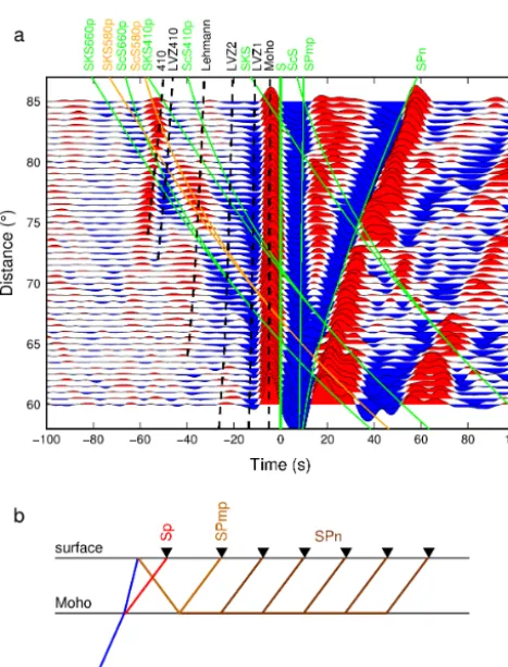
Figure 3. (a) Display of binned S-receiver functions as a function of the epicentral distance. Each bin contains more than one thou-sand traces. Precursors of the S phase from S-to-P conversions in the upper mantle are marked with dashed black lines (410 conver-sion at the 410, LVZ410 converconver-sion at a velocity reduction directly above the 410, Lehmann–Lehmann discontinuity, LVZ1, LVZ2 con-versions at velocity reductions between Moho and Lehmann, Moho conversion at the Moho). LVZ2 and Lehmann are more clear in Fig. 4; they are marked here for comparison. Additional theoretical travel-time curves of ScS, SKS, S-to-P conversions of ScS and SKS at the 410 and 660 discontinuities and at a possible discontinuity at 580 km depth (ScS410p, ScS580p, ScS660p, SKS410p, SKS580p, SKS660p), crustal multiples (SPmp) and SPn are marked in green. (b) Ray paths of Sp, SPmp and SPn.
cursors of all available data in different graphical presen-tations. The data in most of the following figures are low-pass-filtered with 8 s corner period. In Fig. 3a all traces are shown as a function of the epicentral distance. The traces are summed within 0.5◦windows of epicentral distance dis-regarding the back azimuth and station location. The same data are shown in Fig. 4 as common conversion point (CCP) stacks and as a function of the station locations. Distance (or slowness) moveout-corrected traces (reference slowness 6.4 s degree−1) are summed, with hypothetical S-to-P pierc-ing points at 200 km depth within a certain geographical box. The back azimuth of the sources is disregarded. The boxes are aligned along west–east and south–north profiles. West– east profiles are shown in Fig. 4a. The box size is 0.5◦
longi-Figure 4. Display of binned S-receiver function traces along a (a) west–east and (b) south–north line. LVZ1 is the LAB in the western United States and the MLD in the central US. Details of LVZ1 and LVZ2 are shown in the narrower profiles in Figs. 8 and 9. “Lehmann” indicates the bottom of the asthenosphere, and LVZ410 marks a velocity drop above the 410 km discontinuity. Note that this discontinuity is only weakly observed at the eastern end of the line. “410” is the discontinuity at 410 km depth. Although these disconti-nuities are greatly averaged in this display, they appear very clearly.
tude and extends in the south–north direction over the entire array. South–north profiles are shown in Fig. 4b. The box size is 1◦ latitude and extends in west–east direction also over the entire array. In Fig. 5 the traces are shown from the cratonic part of the network (east of 110◦W longitude) as a function of the back azimuth. There is no overlapping of windows. Neighboring stacked traces therefore do not con-tain any common traces.
Figure 5. Display of binned S-receiver functions as a function of the back azimuth (see Fig. 2) of the source of each record, inde-pendent of epicentral distance. Only stations on the cratonic part of the United States (east of 110◦W) are used. The same phases as in Fig. 4 are marked. Most phases do not show any clear dependence on the back azimuth. The only exception might be the 410 discon-tinuity, which is strongest for sources in the northwest quadrant.
“410”), a red discontinuity marked “Lehmann” and an-other blue discontinuity following closely the 410 signal and marked “LVZ410”. The Moho is not the focus of our study. The LVZ410 is observed in P- and S-receiver functions by a number of authors in different parts of the world (e.g., by Schaeffer and Bostock, 2010, in northwestern Canada; by Vinnik et al., 2010, in California and globally by Tauzin et al., 2010). It is interpreted by the presence of water causing partial melt. Jordan and Paulson (2013) discuss the role of this discontinuity for decoupling the thick continental tec-tosphere (which extends below the LAB) from the convect-ing mantle. The Lehmann discontinuity is widely considered as the bottom of the asthenosphere. A global study of the Lehmann discontinuity is given by Gu et al. (2001).
Theoretical travel-time curves of S precursors at the above mentioned discontinuities are marked by dashed black lines in Fig. 3a. They are computed using the IASP91 global refer-ence model with three negative discontinuities (LVZ1, LVZ2 and LVZ410 at 90, 170 and 380 km depth, respectively) and one positive discontinuity (Lehmann at 270 km) added. The Moho is set at 35 km depth. LVZ1 and the 410 are clearly observed in Figs. 3–5. The LVZ2 and the Lehmann disconti-nuity are better observed in Fig. 4.
Additional seismic phases, besides the ones discussed so far, are only visible in Fig. 3a but not in Figs. 4 and 5. The-oretical travel-time curves have been computed to explain these phases. They are marked in green. We see clear nega-tive SKS660p and ScS660p phases from the 660 km discon-tinuity cutting through all other phases prior to the S arrival. These phases are strong at 68–73◦and 75–79◦epicentral
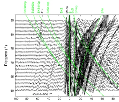
dis-Figure 6. Theoretical seismograms (vertical component) computed with the reflectivity method for comparison with the observed data in Fig. 3a. The strong SPn phase after S agrees well with the data in Fig. 3a. A disagreement between computed and observed seis-mograms is the source-side Pn in front of the S signal (this figure) which is not in the data (Fig. 3a). This is a phase traveling as P along the surface on the source side and is continuously radiating S waves downward. At the receiver side these phases are converted back to P and travel again horizontally along the uppermost mantle and are observed on the vertical component. These phases are not observed in the real data probably because of heterogeneities in the real Earth.
tances and 10–30 s precursor time, and at 75–80◦epicentral distance and 40–50 s precursor time, where they cut through the LVZ2 and the LVZ410 signals. However, the signals are caused by the SKS and ScS conversions at the 410 and 660 discontinuities and have very different slownesses than the S phase. This is the reason why they are canceled out in the moveout-corrected and stacked signals in Figs. 4 and 5. There are also surprisingly clear phases after the S signal in Fig. 3a. They are the crustal multiples SPmp and SPn below the stations (see the ray path of SPn in Fig. 3b), which are so far not much used to infer information about the P velocity below the stations.
the-962 R. Kind et al.: Structure of the upper mantle from USArray S-receiver functions
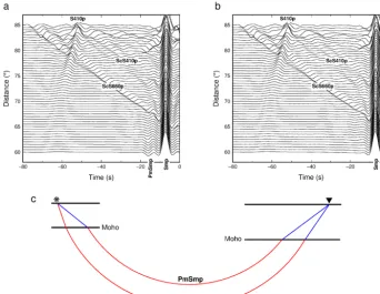
Figure 7. Theoretical seismograms for different structures at the source and receiver sides. (a) Moho is at 50 km depth at the source side, (b) no crust at the source side. Moho depth is 40 km at the receiver side in both cases. The source crust causes a negative precursor before the receiver side S-to-P conversion at the Moho (see PmSmp ray path in c), which could be mistaken as an indication of a velocity drop in the mantle below the Moho. Such phases will only be a problem in interpretations of single data traces. In receiver function processing of real data this should not be a problem since source side models and source depths are different for each record and these effects are erased by summation. (c) Ray paths of Smp and PmSmp.
oretical seismograms, which cause a high noise level in front of the S phase making it difficult to obtain good S precursors. An approximated spike was used as the source time function. The strong SPn and SsPmp phases after S agree well with the data in Fig. 3a. A disagreement between computed and ob-served seismograms is the source-side Pn in front of the S signal (Fig. 6), which is not in the data (Fig. 3a). This is a phase traveling as P along the surface on the source side and continuously radiating S waves downward. At the receiver side these phases are converted back to P and travel again horizontally along the surface. These phases are not observed in the stacked S-receiver functions (Fig. 3a) because of stack-ing of records from many regions with different structures and source depths. The same phases marked green in the data (Fig. 3a) are also marked green in the theoretical seis-mograms in Fig. 6. Note that the IASP91 model has neither an upper-mantle low-velocity zone, the Lehmann discontinu-ity, nor the negative discontinuity above the 410. Therefore these phases are not computed.
In order to point out another possible source of disturb-ing S precursors, we have computed theoretical seismograms similar to Fig. 6 for different crustal models at the source and receiver sides (see Fig. 7). A narrower slowness integration window was used, which excludes source-side Pn. There is a
50 km thick crust at the source side in Fig. 7a and no crust is included at the source side in Fig. 7b. Receiver-side crust is in both cases 40 km thick. The rotated L component is shown, which carries practically only P energy. We see ScS and SKS conversions at the 410 and 660 discontinuities, which cross the Sp conversions at the Moho and at the 410. In Fig. 7c ray paths of Smp with a conversion at the receiver-side Moho (Fig. 7b) and of PmSmp with an additional P-to-S conversion at the source-side Moho (Fig. 7a) are shown. The PmSmp phase is visible in Fig. 7a as a negative precursor of the Moho conversion, which might be mistaken in the real data as a S-to-P conversion at a negative discontinuity below the Moho underneath the station. In receiver functions, however, this phase is reduced due to summation of many events with dif-ferent source depths and source-side structures. Care should be taken if single seismograms are used because it seems im-possible to identify all phases uniquely in these cases.
4 Topography of the discontinuities in the mantle lithosphere
Figure 8.
depth-migrated profiles and in Figs. 10 and 11 several pro-files in the time domain. The width of the propro-files is two de-grees or more of latitude or longitude. The profiles cannot be chosen much narrower because the number of traces avail-able for summation would be too small. Each of the traces in Figs. 10 and 11 was obtained by summation of several hundred traces. The depth domain profiles are chosen along great circles and the time domain data along latitude and lon-gitude. The traces in the time domain profiles (Figs. 10 and
964 R. Kind et al.: Structure of the upper mantle from USArray S-receiver functions
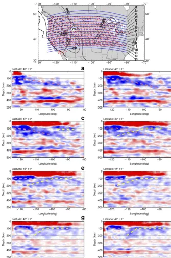
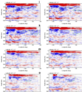
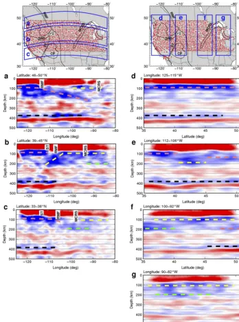
Figure 8. Depth-migrated west–east S-receiver function profiles (see location map at the top of the figure). The width of each profile is 2◦ latitude with 1◦overlap. The latitude of the profiles is marked at each profile. The magenta dashed line is interpreted as the LAB of the Farallon plate, the yellow dashed line as the MLD and the green dashed line as the LAB of the Laurentia plate, respectively. The dashed black line is a low-velocity zone above the 410 discontinuity. See text for a discussion of these discontinuities.
below the Moho we observe several clearly correlatable blue signals (velocity decrease downward). We interpreted these signals as being caused by the LAB in the western United States (marked with magenta lines) and the MLD in the cen-tral United States (marked with yellow lines) and the cratonic LAB in the eastern United States (marked with green lines). In the following we discuss the topography of each of these negative discontinuities in the mantle lithosphere.
4.1 Structure of the western LAB
North of about 46◦N the western LAB extends from the west coast to at least 100◦W where it ends (Figs. 8a–d and 9a). In the wider profile of Fig. 9a it even seems to extend to 90◦W. It is smoothly dipping from about 100 km depth at the west coast to about 200 km depth at its eastern end. Between 46
and 48◦N the depth domain Fig. 8c is not in very good agree-ment with the time domain Fig. 10 (46–48◦N). The reason could be that Fig. 8c has more traces in the north because it follows the great circle. The western LAB is laterally very heterogeneous just north of about 45◦N (see Fig. 10; 46– 48 and 43-46◦N). South of about 45◦N the western LAB reaches from about 114 to about 104◦W with increasing easterly extension towards the south. There is some indica-tion of a local easterly dip also in this part of the western LAB (see Fig. 8l).
Figure 9. The same data and same correlation marks as in Fig. 8 but summed along broader south–north and west–east profiles. The profile width and orientation is shown in the location maps at the top of the figure. Region (a) (northernmost west–east profile) does not have any stations in Canada. However, due to the shallow incidence angle of the S-receiver functions, the mantle below southern Canada is also sampled by events from the northwest. The westernmost south–north profile (d) shows only the western LAB in the mantle lithosphere. In profile (e) we see at the southern and northern ends the western LAB, and in the central part the deep MLD. In profile (f) we see the cratonic MLD (yellow), the cratonic LAB (green) and in the north the deep western LAB (magenta). In the easternmost south–north profile (g) we see the MLD and weakly the cratonic LAB. See Fig. 1 for explanation of the abbreviations of tectonic units.
4.2 The structure of the MLD
The MLD is marked yellow in the figures and it is visible in most profiles in the central United States near 100 km depth where it is expected. It is poorly seen south of about 37◦N, which is probably due to insufficient data (Fig. 8m–p).
966 R. Kind et al.: Structure of the upper mantle from USArray S-receiver functions
an extension of the western LAB or MLD (see Fig. 9b and e). The westerly dip of the MLD is clearer in Fig. 10 (41– 43◦N). There are similar indications in the profile in Fig. 10 (38–41◦N). In Fig. 10 (43–46◦N) it may also be visible, al-though in this profile there is additionally an indication of the east-dipping western LAB. This apparent crossing of discon-tinuities could be caused by lateral variations within the 3◦ latitude wide profile. The observation of such a west-dipping structure in the mantle lithosphere in this part of the United States seems to be new to our knowledge. We will return to this question below when Fig. 11 is discussed.
4.3 The structure of the cratonic LAB
The signals we interpreted as cratonic LAB near 200 km depth are marked green in Figs. 8, 9 and 10. These signals are relatively weak in some of the narrow profiles in Fig. 8. In the wider profiles in Fig. 9c, f and g, the cratonic LAB signals are clearer. In the time domain data in Fig. 10 (33–38◦N) we see a very strong cratonic LAB separated by a sharp step from the western LAB. In Fig. 10 (38–41◦N) the cratonic LAB is also clearly visible. In this 3◦ latitude wide profile we find also indications of the west-dipping MLD, which suggests strong heterogeneities here. Our observations of the cratonic LAB indicate, together with other S-receiver function obser-vations (Miller and Eaton, 2010, in Canada and Kind et al., 2013, in Scandinavia), that the deep cratonic LAB is visible in converted waves. A study of the complete USArray data in the east is required for a more comprehensive analysis of the cratonic LAB. Close to the east coast the LAB again seems to occur near 100 km depth (Rychert et al., 2007).
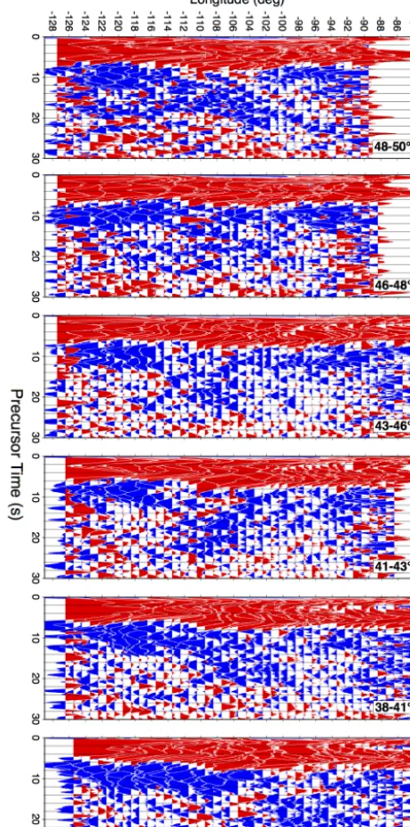
4.4 View on the discontinuities with unfiltered S-receiver functions (Fig. 11)
In Fig. 11 the same data are shown as in Fig. 10, except that no filter is applied apart from the deconvolution. The data are much shorter period than in Fig. 10. If a discontinuity is sharp we expect that its signal also becomes sharper if a shorter period filter or no filter is applied. This seems not to be the case for all the upper mantle discontinuities ob-served in this study such as the western and cratonic LAB and MLD. The discontinuities seem to dissolve in a sequence of sharper discontinuities with a very scattered appearance with sometimes a relatively short correlation length. A kind of scattered lamella structure with stepwise decreasing ve-locity could cause such signals. This means that these dis-continuities are in reality transition zones with stepwise de-creasing velocities. A lamella structure of the upper mantle has been observed in long-range controlled source profiles for a long time, for example in Phanerozoic western Europe (see Kind, 1974) and in the cratons of northern Eurasia (see Mechie et al., 1993) and North America (see Thybo and Per-chuc, 1997). No phases are marked in Fig.11 in order not to bias the reader. Generally the same phases as in Fig. 10 are
also visible in Fig. 11, however, as groups of scattered sig-nals. The signal with the largest amplitudes is the western LAB, especially in Fig. 11 (33–38◦N). It spreads out over more than 5 s, which corresponds to at least 50 km. We see in Fig. 11 (48–50◦N) the east-dipping western LAB reach-ing far below the MLD. West-dippreach-ing structures are visible in Fig. 11 (43–46◦N) and especially clearly in Fig. 11 (41– 43◦N). The connection between these structures and the cra-tonic MLD seems obvious. As in the north, indications of an east-dipping structure are also observed in Figs. 8l and 11 (38–41◦N) and. The sharp step between the western LAB and cratonic LAB near 105◦W is also clear in the unfiltered data in Fig. 11 (33–38◦N) as in the longer period filtered data in Fig. 10 (33–38◦N).
How do our observations agree with earlier seismic im-ages of the mantle lithosphere in the western and central US? Levander and Miller (2012) also used S-receiver func-tion data from USArray in the same area. They also observe the break in the LAB along the Sevier thrust belt. However they interpret the deep velocity drop east of the Sevier thrust belt as the cratonic LAB of the Laurentia plate. They do not report on the MLD and a west-dipping structure between the Rocky Mountain Front and the Sevier thrust belt. Hopper et al. (2014) observed in the Yellowstone region the same break in the mantle lithosphere, also using S-receiver functions. They observed east of Yellowstone a faint shallow MLD but no west-dipping structure. Hansen et al. (2013) observed the LAB below the Colorado Plateau at 100–150 km depth and east of it at 150–200 km depth. This agrees with our LAB observations along 38◦N (Fig. 8l). Foster et al. (2014) also studied the lithosphere in the American Midwest with USAr-ray S-receiver functions. They observed east of about 98◦W a strong MLD near 100 km depth and the cratonic LAB at 200–250 km depth. Their data are close to our profile shown in Fig. 8d. We also see here a strong MLD east of about 98◦W. However we see, in addition, indications of the east-dipping LAB and the west-east-dipping MLD within the 2◦ lat-itude wide profile in Fig. 8d. Lekic and Fischer (2014) ob-served below the Colorado Plateau and surroundings scat-tered negative signals near 100 km depth in S-receiver func-tions which they interpreted as the LAB beneath the Basin and Range Province and the Rocky Mountain Front, west and east of the Colorado Plateau, respectively. Beneath the stable Colorado Plateau and the Great Plains they interpreted a negative phase in the same depth range as the MLD. We observe below the Colorado Plateau the LAB of the western United States at about 100 km depth (Fig. 9c).
5 Anisotropy of the MLD?
Figure 10. West–east S-receiver function profiles in the time do-main. The latitude of the distribution of piercing points in 200 km depth is marked in each panel. The data are filtered with an 8 s low-pass filter. Correlated phases are marked with the same colors as in Figs. 8 and 9, except that here black represents the LAB of the Juan de Fuca plate.
The MLD in our data does not show any sign change or sig-nificant change of the amplitudes as a function of the back azimuth (see LVZ1 in Fig. 5). This means that there are no indications in our data for azimuthal anisotropy as the cause of the MLD signal in the cratonic US. The azimuthal cov-erage of seismic sources is good for the identification of
az-Figure 11. The same profiles as in Fig. 10 but with no filter applied.
968 R. Kind et al.: Structure of the upper mantle from USArray S-receiver functions
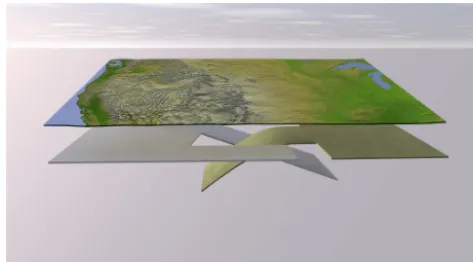
Figure 12. Visualization of the interfingering of the colliding Far-allon LAB in the west with the Laurentia MLD in the east. The cratonic LAB is left out of the figure. The profiles in Figs. 9a, b, c and 10 (48–50, 41–43, and 33–38◦N) represent the east-dipping part of the Farallon LAB in the north, the west-dipping Laurentia MLD and the flat part of the far-east-reaching Farallon plate in the south. The lateral transition between these three parts is in reality not as sharp as indicated here, but much more heterogeneous.
6 Low-velocity zone above the 410 km discontinuity
Tauzin et al. (2010) observed a nearly global velocity reduc-tion at about 350 km depth without any relareduc-tion to surface tectonics. The cause of this low-velocity layer is thought to be partial melt caused by dehydration (Bercovici and Karato, 2003). We observed a similar discontinuity in the USAr-ray S-receiver functions (see, e.g., Figs. 4 and 9). Jordan and Paulson (2013) suggested that a low-viscosity zone di-rectly above the 410 discontinuity decouples the thick cra-tonic tectosphere from the flowing mantle. Looking at Fig. 9 it seems that the strongest signals of the phase LVZ410 are observed in the western United States where the LAB oc-curs at about 100 km depth. The signal is weaker in the cra-tonic United States (Fig. 9b, c, g). This means that the veloc-ities directly above the 410 are lower in Phanerozoic regions than in cratonic regions of the US. This supports the tomo-graphic results summarized by Jordan and Paulson (2013) of the cratonic tectosphere having higher velocities down to the 410 km discontinuity.
7 Conclusions
We have been able to image with S-receiver functions the major seismic discontinuities in the upper mantle below large regions of the western and central United States. In the upper 200 km we see complex structures of the western LAB and the MLD (Fig. 12). The east-dipping LAB interferes with the west-plunging MLD in a complicated manner. We inter-pret these structures as being caused by the continental colli-sion of the Farallon plate and the Laurentia plate. The MLD appears to be deformed in this collision in a similar way as could be expected for a shallow non-cratonic LAB. This
could mean that the Archean lithosphere of the craton (Yuan and Romanowicz, 2010) was deformed during the collision with the Farallon plate. The western LAB dips partly far to the east to the mid-continental rift system, where it could be mistaken for the cratonic LAB. The deep cratonic LAB near 200 km depth is weakly observed at the eastern end of the considered area (from about 90–82◦W). Its connection to the previously observed shallow LAB near the Atlantic coast needs further investigation with all eastern USArray data. The cratonic LAB is very strong in the south-western part of the US. Below 200 km depth we have observed a scattered Lehmann discontinuity, which is considered to be the bottom of the asthenosphere. Directly above the 410 km discontinu-ity mainly in the western United States we observed a strong velocity reduction. Such a velocity reduction directly above the 410 is not observed in the cratonic US, which indicates higher velocity here.
Acknowledgements. This research was supported by the Deutsche Forschungsgemeinschaft. The facilities of the IRIS Data Manage-ment System, and specifically the IRIS Data ManageManage-ment Center, were used for access to waveform and metadata required in this study (http://ds.iris.edu/data/). The IRIS DMS is funded through the National Science Foundation and specifically the GEO Directorate through the Instrumentation and Facilities Program of the National Science Foundation under Cooperative Agreement EAR-1063471. We also wish to thank Gene Humphreys and Shun Karato for discussions, and Theresia Ziegs and Irene Kind for help in the data processing. Finally we would like to thank Barbara Romanowicz and an anonymous reviewer for their very helpful comments.
The article processing charges for this open-access publication were covered by a Research
Centre of the Helmholtz Association.
Edited by: J. Plomerova
References
Abt, D. L., Fischer, K. M., French, S. W., Ford, H. A., Yuan, H., and Romanowicz, B.: North American lithospheric discontinuity structure imaged by Ps and Sp receiver functions, J. Geophys. Res., 115, B09301, doi:10.1029/2009JB006914, 2010.
Barrell, J.: The strength of the Earth’s crust, J. Geol., 22, 655–683, 1914.
Bercovici, D. and Karato, S.: Whole mantle convection and transition-zone water filter, Nature, 425, 39–44, 2003.
Bock, G.: Multiples as precursors to S, SKS and ScS, Geophys. J. Int., 119, 421–427, 1994.
rounding oceans, J. Geophys. Res., 99, 11591–11621, 1994. Gu, J. Y., Dziewonski, A. M., and Ekström, G.: Preferential
detec-tion of the Lehmann discontinuity beneath continents, Geophys. Res. Lett., 28, 4655–4658, 2001.
Hansen, S., Dueker, K., Stachnik, J., Aster, R., and Karl-strom, K. A.: A rootless rockies – support and lithospheric struc-ture of the Colorado Rocky Mountains inferred from CREST and TA seismic data, Geochem. Geophy. Geosy., 14, 2670–2695, doi:10.1002/ggge.20143, 2013.
Hopper, E., Ford, H. E., Fischer, K. M., and Lekic, V.: The lithosphere-asthenosphere boundary and the tectonic-magmatic history of the northwestern United States, Earth Planet. Sc. Lett., 402, 69–81, 2014.
Jones, C. H. and Phinney, R. A.: Seismic structure of the lithosphere from teleseismic converted arrivals observed at small arrays in the southern Sierra Nevada and vicinity, California, J. Geophys. Res., 103, 10065–10090, doi:10.1029/97JB03540, 1998. Jordan, T. H.: The continental tectosphere, Rev. Geophys. Space
Ge., 13, 1–12, 1975.
Jordan, T. H. and Paulson, E. M.: Convergence depths of tectonic regions from an ensemble of global tomographic models, J. Geo-phys. Res.-Sol. Ea., 118, 4196–4225, doi:10.1002/jgrb.50263, 2013.
Karato, S.: The origin of the asthenosphere, Earth Planet. Sc. Lett., 321–322, 95–103, doi:10.1016/j.epsl.2012.01.001, 2012. Kind, R.: Long range propagation of seismic energy in the lower
lithosphere, J. Geophys., 40, 189–202, 1974.
Kind, R.: The reflectivity method for different source and receiver structures, J. Geophys., 58, 146–152, 1985.
Kind, R., Yuan, X., and Kumar, P.: Seismic receiver functions and the lithosphere-asthenosphere boundary, Tectonophysics, 536– 537, 25–43, doi:10.1016/j.tecto.2012.03.005, 2012.
Kind, R., Sodoudi, F., Yuan, X., Shomali, H., Roberts, R., Gee, D., Eken, T., Bianchi, M., Tilmann, F., Balling, N., Ja-cobsen, B. H., Kumar, P., and Geissler, H. W.: Scandinavia: a former Tibet?, Geochem. Geophy. Geosy., 14, 4479–4487, doi:10.1002/ggge.20251, 2013.
Kosarev, G., Kind, R., Sobolev, S. V., Yuan, X., Hanka, W., and Oreshin, S.: Seismic evidence for detached Indian lithospheric mantle beneath central Tibet, Science, 283, 1306–1308, 1999. Kumar, P., Kind, R., and Yuan, X. H.: Receiver function
summa-tion without deconvolusumma-tion, Geophys. J. Int., 180, 1223–1230, doi:10.1111/j.1365-246X.2009.04469.x, 2010.
discontinuity structure in the western US, Geochem. Geophy. Geosy., 13, Q0AK07, doi:10.1029/2012GC004056, 2012. Li, X., Yuan, X. H., and Kind, R.: The lithosphere–asthenosphere
boundary beneath the western United States, Geophys. J. Int., 170, 700–710, doi:10.1111/j.1365-246X.2007.03428.x, 2007. Mechie, J., Egorkin, A. V., Fuchs, F., Ryberg, T., Solodilov, L.,
and Wenzel, F.: P-wave mantle velocity structure beneath north-ern Eurasia from long-range recordings along the profile Quartz, Phys. Earth Planet. Inter., 79, 269–286, 1993.
Miller, M. S. and Eaton, D. W.: Formation of the cratonic mantle keels by accreation: evidence from S receiver functions, Geo-phys. Res. Lett., 37, L18305, doi:10.1029/2010GL044366, 2010. Rychert, C., Fischer, K., and Rondenay, S. A.: A sharp lithosphere– asthenosphere boundary imaged beneath eastern North America, Nature, 436, 542–547, doi:10.1038/nature03904, 2005. Rychert, C. A. and Shearer, P. M.: A global view of the
lithosphere-asthenosphere boundary, Science, 324, 495–498, 2009. Rychert, C. A., Shearer, P. M., and Fischer, K. M.: Scattered wave
imaging of the lithosphere–asthenosphere boundary, Lithos, 120, 173–185, doi:10.1016/j.lithos.2009.12.006, 2010.
Rychert, K., Rondenay, S., and Fischer, K.: P-to-S and S-to-P imaging of a sharp lithosphere–asthenosphere boundary be-neath eastern NorthAmerica, J. Geophys. Res., 112, B08314, doi:10.1029/2006jb004619, 2007.
Schaeffer, A. J. and Bostock, M. G.: A low-velocity zone atop the transition zone in northwestern Canada, J. Geophys. Res., 115, B06302, doi:10.1029/2009JB006856, 2010.
Schmandt, B. and Humphreys, E.: Seismically imaged relict slab from the 55 Ma Siletzia accretion to the northwest United States, Geology, 39, 175–178, doi:10.1130/G31558.1, 2011.
Schmandt, B. and Lin. F.-C.: P and S wave tomography of the man-tle beneath the United States, Geophys. Res. Lett., 41, 6342– 6349, doi:10.1002/2014GL061231, 2014.
Selway, K., Ford, H., and Kelemen, P.: The seismic mid-lithospheric discontinuity, Earth Planet. Sc. Lett., 414, 45–57, doi:10.1016/j.epsl.2014.12.029, 2015.
Shearer, P. M.: Constraints on upper mantle discontinuities from ob-servations of long-period reflected and converted phases, J. Geo-phys. Res., 96, 18147–18182, 1991.
970 R. Kind et al.: Structure of the upper mantle from USArray S-receiver functions
Sigloch, K., McQuarrie, N., and Nolet, N.: Two-stage subduction history under North America inferred from multiple-frequency tomography, Nat. Geosci., 1, 458–462, doi:10.1038/ngeo231, 2008.
Sodoudi, F., Yuan, X., Kind, R., Lebedev, S., Adam, J. M.-C., Käs-tle, E., and Tilmann, F.: Seismic evidence for stratification in composition and anisotropic fabric within the thick lithosphere of Kalahari Craton, Geochem. Geophy. Geosy., 14, 5393–5412, doi:10.1002/2013GC004955, 2013.
Tauzin, B., Debayle, E., and Wittlinger, G.: Seismic evidence for global low-velocity layer within the Earth’s upper mantle, Nat. Geosci., 3, 718–721, doi:10.1038/NGEO969, 2010.
Thybo, H. and Perchuc, E.: The seismic 8 degrees discontinuity and partial melting in continental mantle, Science, 275, 1626–1629, 1997.
Vinnik, L., Ren, Y., Stutzmann, E., Farra, V., and Kise-lev, S.: Observations of S410p and S350p phases at seismo-graph stations in California, J. Geophys. Res., 115, B05303, doi:10.1029/2009JB006582, 2010.
Wilson, D. C., Angus, D. A., Ni, J. F., and Grand, S. P.: Constraints on the interpretation of S-to-P receiver functions, Geophys. J. Int., 165, 969–980, 2006.
Yoshizawa, K.: Radially anisotropic 3-D shear wave structure of the Australian lithosphere and asthenosphere from multi-mode surface waves, Phys. Earth Planet. In., 235, 33–48, doi:10.1016/j.pepi.2014.07.008, 2014.
Yuan, H. Y. and Romanowicz, B.: Lithospheric layering in the North American craton, Nature, 466, 1063–1071, doi:10.1038/nature09332, 2010.
Yuan, H., Romanowicz, B., Fischer, K., and Abt, D.:3-D shear wave radially and azimuthally anisotropic velocity model of the north American upper mantle, Geophys. J. Int., 184, 1237–1260, doi:10.1111/j.1365-246X.2010.04901.x, 2011.
Yuan, X., Ni, J., Kind, R., Mechie, J., and Sandvol, E.: Lithospheric and upper mantle structure of southern Tibet from a seismolog-ical passive source experiment, J. Geophys. Res., 102, 27491– 27500, 1997.
Yuan, X., Kind, R., Li, X., and Wang, R.: The S receiver func-tions; synthetics and data example, Geophys. J. Int., 165, 555– 564, doi:10.1111/j.1365-246X.2006.02885.x, 2006.