https://doi.org/10.5194/soil-5-275-2019
© Author(s) 2019. This work is distributed under the Creative Commons Attribution 4.0 License.
SOIL
Error propagation in spectrometric functions
of soil organic carbon
Monja Ellinger1, Ines Merbach2, Ulrike Werban3, and Mareike Ließ1 1Department of Soil System Science,
Helmholtz Centre for Environmental Research – UFZ, Halle (Saale), Germany 2Department of Community Ecology,
Helmholtz Centre for Environmental Research – UFZ, Bad Lauchstädt, Germany 3Department of Monitoring and Exploration Technologies,
Helmholtz Centre for Environmental Research – UFZ, Leipzig, Germany
Correspondence:Mareike Ließ ([email protected])
Received: 30 November 2018 – Discussion started: 23 January 2019 Revised: 9 August 2019 – Accepted: 29 August 2019 – Published: 25 September 2019
Abstract. Soil organic carbon (SOC) plays a major role concerning chemical, physical, and biological soil properties and functions. To get a better understanding of how soil management affects the SOC content, the precise monitoring of SOC on long-term field experiments (LTFEs) is needed. Visible and near-infrared (Vis– NIR) reflectance spectrometry provides an inexpensive and fast opportunity to complement conventional SOC analysis and has often been used to predict SOC. For this study, 100 soil samples were collected at an LTFE in central Germany by two different sampling designs. SOC values ranged between 1.5 % and 2.9 %. Regression models were built using partial least square regression (PLSR). In order to build robust models, a nested repeated 5-fold group cross-validation (CV) approach was used, which comprised model tuning and evaluation. Various aspects that influence the obtained error measure were analysed and discussed. Four pre-processing methods were compared in order to extract information regarding SOC from the spectra. Finally, the best model perfor-mance which did not consider error propagation corresponded to a mean RMSEMVof 0.12 % SOC (R2=0.86). This model performance was impaired by1RMSEMV=0.04 % SOC while considering input data uncertainties (1R2=0.09), and by1RMSEMV=0.12 % SOC (1R2=0.17) considering an inappropriate pre-processing. The effect of the sampling design amounted to a1RMSEMVof 0.02 % SOC (1R2=0.05). Overall, we empha-size the necessity of transparent and precise documentation of the measurement protocol, the model building, and validation procedure in order to assess model performance in a comprehensive way and allow for a com-parison between publications. The consideration of uncertainty propagation is essential when applying Vis–NIR spectrometry for soil monitoring.
1 Introduction
Soil is at the same time one of the most important and one of the most limited natural resources. Most of all, it is needed for food production, as well as for the production of energy crops and fibre, and for the provision of freshwater (John-son, 2008; Lorenz and Lal, 2016). All these aspects depend on the quality of the soil, which is determined by its site-specific properties. And this quality, in turn, is much influ-enced by its soil organic carbon (SOC) content since it affects
carbon (Stockmann et al., 2011), achieving both food secu-rity and a strategy against the increasing CO2concentration in the atmosphere (Lal, 2004; Lorenz and Lal, 2016; McBrat-ney et al., 2014). As the SOC content of soils reacts very slowly to environmental changes (Meersmans et al., 2009), long-term field experiments (LTFEs) are required to under-stand the impact of soil management and farming systems on the rate of SOC sequestration (Lal, 2004), as well as on yield and crop quality in the long run.
The precise monitoring of SOC on an LTFE with con-ventional laboratory analysis is labour- and cost-intensive (Adamchuk and Viscarra Rossel, 2010; Loum et al., 2016) as it requires the analysis of a rather high number of samples. Visible and near-infrared (Vis–NIR) reflectance spectrome-try can facilitate this procedure. It is non-destructive, fast, and economical (Mouazen et al., 2010) and requires the con-ventional laboratory analysis to be conducted on only a small number of soil samples, as well as little sample preparation (Conforti et al., 2015). The obtained spectrum contains infor-mation about many different soil components (Conforti et al., 2015; Viscarra Rossel et al., 2006b); please compare Sten-berg et al. (2010) for a review on the past and current role of Vis–NIR spectrometry in soil science. Spectral absorption features are caused by vibrational stretching and bending of structural molecule groups and electronic excitation (Ben-Dor et al., 1999; Dalal and Henry, 1986). Molecule vibrations from hydroxyl, carboxyl, and amine functional groups pro-duce absorption features related to soil organic matter in the mid-infrared (MIR) region of the spectra (Croft et al., 2012). In comparison, Vis–NIR spectra show only broad and un-clear adsorption features related to overtone vibrations from the MIR, but instruments are less cost-intensive and available for field monitoring as well (Stenberg and Viscarra Rossel, 2010; Viscarra Rossel et al., 2006a). Furthermore, in diffuse reflectance spectroscopy, scattering properties depend on the particular wavelengths and can vary significantly over the Vis–NIR spectral range (Pilorget et al., 2016). Hence, the pre-processing of Vis–NIR spectra is necessary in order to extract soil property-related information (Stenberg and Vis-carra Rossel, 2010). As there is no standard pre-processing technique which works on all spectral data (Stenberg and Viscarra Rossel, 2010), it is recommended to always test var-ious techniques and to choose the one which performs best for the respective data. Several studies, therefore, have com-pared a rather high number of pre-processing methods. Scat-tering and other effects attributed to within-sample variance can be addressed by repeated measurements of replicate sam-ples (e.g. Pimstein et al., 2011). Altogether, Vis–NIR soil spectrometry has been used on many occasions to build SOC prediction models (Jiang et al., 2016; Kuang and Mouazen, 2013; Nocita et al., 2013).
However, the application of Vis–NIR soil spectrometry for SOC determination involves a couple of uncertainties. The required calibration data are determined with standard labo-ratory analysis, e.g. dry combustion, with associated
uncer-tainties. On the other hand, the spectral measurements are af-fected by the sample preparation, e.g. drying, sieving, grind-ing (e.g. Nduwamungu et al., 2009). Furthermore, sensor noise and other spectrometer internal sources (electronic and mechanical) can affect the measurements (Schwartz et al., 2011). Finally, these two uncertain data sources are related by a regression model. And the model building procedure in-volves a couple of error sources itself. The development of robust models requires a resampling procedure to determine the model parameters and to avoid overfitting; the applied re-sampling method impacts model performance (e.g. Molinaro et al., 2005; Beleites et al., 2005). Further aspects that im-pact model performance are the available dataset in concor-dance with the applied sampling design, the handling of out-liers, spectral pre-processing, and last but not least the model evaluation procedure. In most studies dealing with SOC pre-diction from Vis–NIR spectra, no clear statement about in-put data uncertainties or their handling is made. The reported prediction errors only refer to the model building procedure, while uncertainties from laboratory measurements are ne-glected. Commonly, only a single SOC measurement per soil sample is available, and in spectrometric laboratory measure-ments, the general approach consists in averaging the multi-ple measured spectra of one sammulti-ple to one spectrum, which is then used for model building (Ge et al., 2011; Stevens et al., 2013; Viscarra Rossel et al., 2003). However, the number of measurements used to gain one averaged spectrum differs between studies. Jiang et al. (2016), for example, averaged 10 measurements to receive one spectrum, while Volkan Bilgili et al. (2010) and Wang et al. (2014) used four measurements. This difference is also assumed to have an influence on the uncertainties contained in the input data.
Overall, to allow for comparison between studies, in terms of predictive uncertainty in % SOC, a modelling proce-dure is required that deals with the propagation of the in-put data uncertainties. For discussion of the general concept, please refer to Jansen (1998); for applications in soil mod-elling, compare, for example, Heuvelink (1999) and Pog-gio and Gimona (2014). Although the problem of the in-volved uncertainties in Vis–NIR spectrometry is well-known (e.g. Gholizadeh et al., 2013; Nduwamungu et al., 2009; Mortensen, 2014), implementations of uncertainty propaga-tion in Vis–NIR spectrometric modelling are lacking.
2 Material and methods
2.1 The Static Fertilization Experiment Bad Lauchstädt
charac-terized as a Haplic Chernozem developed from loess (Alter-mann et al., 2005) with a soil texture of 21.1±1.2 % clay, 72.1±1.7 % silt, and 6.9±1.9 % sand (Dierke and Wer-ban, 2013). Saturated water conductivity and air capacity are medium to high in the topsoil (Altermann et al., 2005). The Static Fertilization Experiment was initialized in 1902 by Schneidewind and Gröbler and is about 4 ha in size (Merbach and Schulz, 2013). Its objective is to investigate the impact of organic and mineral fertilization on soil fertility as well as yield and quality of crops (Körschens and Pfefferkorn, 1998; Schulz, 2017). The experiment includes eight subfields with a width from 25.2 to 28.5 m and a length of 190 m which are each divided into 18 plots that are treated with different min-eral and organic fertilizer as well as planted with different crops following a crop rotation (Körschens and Pfefferkorn, 1998). The plots of subfields 4 and 5 are additionally split into 5 smaller subplots.
2.2 Sampling design
A total of 100 soil samples were taken at the soil surface (0–10 cm) in September 2016. The exact location of the sam-pling points was determined by a differential GPS/GNSS Le-ica Viva GS08. It was decided to sample at precise point locations instead of taking samples representative of LTFE plots to allow for a direct comparison with spectrometric field measurements for area-wide regionalization (not included in this study). The sampling points were determined beforehand by two sampling designs. Based on the LTFE treatment fac-tors and per-plot soil archive data includingCorg,Ntot, plant-available P, plant-plant-available K (both with double lactate ex-tract method (VDLUFA, 2012), and pH (Fig. 1), both de-signs strived to select a dataset of 50 samples representative of the soil variability of the entire LTFE. Categorical and continuous data first entered a factor analysis for mixed data (FAMD) performed with R package FactoMineR (Lê et al., 2008) to allow for further joint analysis. For design A the LTFE plots were then grouped by ak-means cluster analysis. R package NbClust (Charrad et al., 2014) automatically de-termines the optimal number of clusters making use of 30 in-dices. In the end, 10 plots were randomly selected from each of the resulting five clusters, making a total of 50 plots to be sampled. For design B, the Kennard–Stone algorithm was applied with R package prospectr (Kennard and Stone, 1969; Stevens and Ramirez Lopez, 2014); 50 LTFE plots were se-lected involving 5 repetitions of the algorithm to reduce inter-point dependence. Finally, one sampling inter-point was randomly selected from each of the 50 LTFE plots for design A and B based on a 5 cm×5 cm raster. Plot margins of 1.5 m (3 m be-tween plots) were excluded. Figure 2 shows the location of the obtained 100 soil samples.
Figure 1.Soil archive data of the LTFE measured from 2004 to 2007 (reports of the experimental station Bad Lauchstädt 2004– 2007; unpublished data).
2.3 Laboratory measurements
The soil samples were air-dried, sieved, and ground prior to carbon measurements with dry combustion. A high-end elemental analyser vario EL cube CN was used. Measure-ments were repeated in three replicate samples. Carbon mea-surements were taken as SOC due to negligibly small car-bonate contents (below detection limit). The Vis–NIR con-tact measurements were performed on air-dried and sieved (2 mm) samples in July 2017, using Veris® Vis–NIR spec-trophotometer by Veris Technologies, Inc. (hereinafter called Veris) containing an Ocean Optics USB4000 instrument (200 to 1100 nm) and a Hamamatsu TG series mini-spectrometer (1100 to 2200 nm, resolution 6 nm). The device was warmed up for at least 20 min before performing measurements. All measurements were taken in a dark room to prevent day-light from affecting the outcome. The soil samples were scanned from the top. Before and between soil sample mea-surements, Veris was calibrated using four Avian Technolo-gies Fluorilon™ grayscale standards. Each soil sample was divided into three subsamples filled into Petri dishes (Schott Duran Petri dishes; Duran Group, Mainz, Germany). These replicate samples were not related to the three replicate sam-ples used for SOC measurements. For each replicate sample, six spectra were gained by measuring each replicate sample three times, rotating it by 90◦, and then measuring it three
times again. This procedure resulted in 18 spectra for each soil sample. Internally the spectrometer averaged 25 scans for each spectrometer reading (spectrometer setting).
2.4 Spectral pre-processing
anal-Figure 2.Site of the Static Fertilization Experiment in Bad Lauchstädt with LTFE plots and sampling points according to design A and B. Plot margins excluded from sampling are visible as 3 m wide stripes between plots.
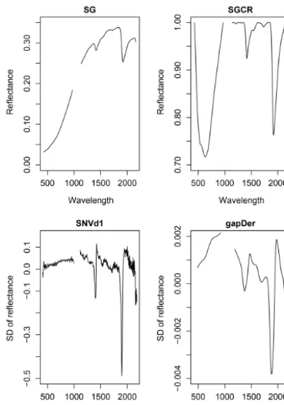
ysis (PCA) is performed, using then the first two obtained PCs for outlier detection with function aq.plot. Out of the tested pre-processing methods, four different combinations are shown in this study in order to demonstrate their impact on model performance. Their application resulted in spectra with different wavelength ranges (Table 1) and different ap-pearance (Fig. 3). These pre-processing techniques include the Savitzky–Golay algorithm (SG), the continuum removal (CR), the standard normal variate (SNV), the first deriva-tive (d1), and the gap-segment algorithm (gapDer). All pre-processing methods for this study were conducted using R package prospectr (Stevens and Ramirez Lopez, 2014). The SG algorithm fits a polynomial regression on the spectral data to find the derivative at a centre point i of a defined smoothing window (w) (Savitzky and Golay, 1964). CR can be seen as a spectra normalization technique which enables the comparison of different absorption characteristics from a mutual baseline. The continuum is calculated by linear in-terpolation of the reflectance spectrum’s maxima. We imple-mented CR following Stevens and Ramirez Lopez (2014) by calculating
φi = xi ci
(1)
fori=1, . . ., p, withxi andci being the initial and the
con-tinuum reflectance values at wavelengthiof a set ofp wave-lengths. φi then gives the continuum-removed reflectance
value. SNV is a scatter-corrective pre-processing method (Barnes et al., 1989). The basic formula is as follows:
xcorr=
xorg−a0 a1
, (2)
wherea0 is the measured spectrum’s average value which shall be corrected, and a1 is the sample spectrum’s stan-dard deviation. xorg is the original spectrum and xcorr the corrected spectrum after applying SNV. In this study, SNV operates row-wise, and each observation is processed on its own (Stevens and Ramirez Lopez, 2014). d1 is calculated by the finite difference method, i.e. the difference between two subsequent data pointsxi andxi−1(Eq. 3):
Figure 3. Impact of different pre-processing techniques on a spectrum; SG−Savitzky–Golay, CR−continuum removal, SNV−standard normal variate, d1−1st derivative, gapDer− gap-segment algorithm.
wherexi0 is the value of the first derivative at theith wave-length (Rinnan et al., 2009). The downside of using deriva-tive spectra is their tendency to increase noise so that smooth-ing of the data is required (Stevens and Ramirez Lopez, 2014). With the gapDer, smoothing is performed under a cho-sen segment size (s) and then a derivative follows (Stevens and Ramirez Lopez, 2014).
2.5 Error propagation
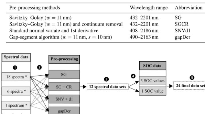
A problem occurring in every model building process is un-certainty propagation. Uncertainties of the input data and model result in uncertainties in the output (Brown and Heuvelink, 2006). Uncertainties in the input data are caused by errors in data acquisition (e.g. measurement errors) as well as variation in the data themselves (e.g. within-sample variability) (Heuvelink, 1999). For this study, there are two different sources for errors in data acquisition: the measure-ment of the spectral data and the measuremeasure-ment of the SOC content of the soil samples. In order to investigate the in-fluence of these errors, different datasets were built in this study. Figure 4 gives an overview. From the measured Vis– NIR spectra, three different spectral data variants were cre-ated (Fig. 4, step 1). For the first variant, all 18 spectra were
retained. The inclusion of all 18 spectra reveals the influence of the error implemented in the spectral measurements as well as the influence of the within-sample variability. For the second variant, the three measurements obtained before and after sample rotation were averaged separately resulting in 6 spectra per sample showing the influence of within-sample variability (replicate measurements). For the third data vari-ant, all 18 spectra were averaged to 1 mean spectrum per sample, removing the influence of the measurement error as well as the within-sample variability. The different spectra obtained through this procedure can be seen in Fig. 5; only parts of the spectra are depicted in order to show their dif-ferences. The three different spectral data variants were then pre-processed with the methods from Table 1 (Fig. 4, step 2), resulting in 12 different spectral datasets (Fig. 4, step 3). These were then combined with single and averaged SOC values in step 4 so that altogether 24 datasets were obtained (Fig. 4, step 5). In order to compare the two sampling de-signs, this procedure was carried out for the 50 soil samples labelled “A” and “B” and also for the complete set of soil samples. In this way, three different soil sample sets (“A”, “B” and “all” samples) were obtained.
2.6 Model building and validation
Regression models were built using partial least square re-gression (PLSR). Out of the many algorithms, PLSR is seen as a standard method for spectral calibration and prediction (Mouazen et al., 2010; Viscarra Rossel et al., 2006b). For re-cent applications to predict SOC from Vis–NIR soil spectra, see e.g. Liu et al. (2018) and Yang et al. (2019). PLSR is described in detail by Martens and Næs (1989) and Naes et al. (2002). It incorporates characteristics from PCA and mul-tiple regression (Abdi, 2007). The concept behind PLSR is to seek a small number of linear combinations (components or latent factors) obtained from the measured spectral data and to use them in the regression equation to predict SOC instead of the initial values (Martens and Næs, 1989; Naes et al., 2002). These components are constructed so that they ac-count for most of the variance in the measured spectral data (X) and the SOC content (Y), and at the same time they max-imize the correlation betweenXandY. In other words, PLSR leads to the covariance betweenX andY being maximized (Bjørsvik and Martens, 2008; Wehrens, 2011).
Table 1.Combinations of pre-processing techniques used in this study;wis window size,ssegment size.
Pre-processing methods Wavelength range Abbreviation
Savitzky–Golay (w=11 nm) 432–2201 nm SG
Savitzky–Golay (w=11 nm) and continuum removal 432–2201 nm SGCR
Standard normal variate and 1st derivative 408–2186 nm SNVd1
Gap-segment algorithm (w=11 nm,s=10 nm) 490–2163 nm gapDer
Figure 4. Datasets to investigate the uncertainty propagation. SG−Savitzky–Golay, CR−continuum removal, SNV−standard normal variate, d1−1st derivative, gapDer−gap-segment algorithm.
parameters (Guio Blanco et al., 2018; Hastie et al., 2009; Kuhn and Johnson, 2013). For small datasets, k-fold cross-validation (CV) is recommended (Hastie et al., 2009).
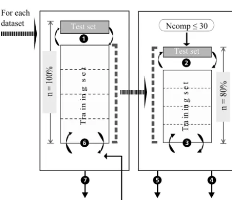
In this study, model building, model validation, and model tuning were implemented using a nested CV approach (Fig. 6; e.g. Varma and Simon, 2006, and Guio Blanco et al., 2018). The CV for model validation and tuning con-sisted of a repeated k-fold group CV. In order to calculate reliable error measures, the subdivision of the spectral data into the folds had to account for repeated scans and repli-cate measurements per sample. Accordingly, all spectra for one sample were assigned to the same fold duringk-fold CV, i.e. k-fold group CV. Furthermore, to allow for comparison of the models built on behalf of the 24 datasets (Fig. 4), the created folds coincide for all datasets; the data of cer-tain sample IDs were always assigned to the same fold ID. For the model validation CV, two further aspects were taken into account that were neglected for the model tuning CV. The group CV was adapted to also guarantee that neighbour-ing points of≤5 m distance were assigned to the same fold to avoid spatial autocorrelation and error measures that are too optimistic. Furthermore, the response variable’s density distribution was taken into account during fold creation, i.e. a stratified CV. Overall, a nested repeatedk-fold group CV was applied. Five repetitions of a 5-fold group CV were con-ducted in this case. Kuhn and Johnson (2013) recommend 5-fold CV as it can increase the precision of the prediction while maintaining a small bias.
Figure 6 shows the various steps of the modelling pro-cedure involving repeated 5-fold group CV for model tun-ing (right box) and validation (left box). In the process, the dataset (n=100 %) is randomly subdivided into 5 folds of
Table 2.Data basis per soil sample.
Number of Number of The resulting
SOC values spectra size of the
per sample per sample dataset
per sample
Dataset111 3 18 54
Dataset101 3 6 18
Dataset100 3 1 3
Dataset011 1 18 18
Dataset001 1 6 6
Dataset000 1 1 1
com-Figure 5.Zoom-in to a sample’s spectral dataset:(a)18 spectra comprised of 6 replicate sample measurements with 3 scans each,(b)6 spec-tra related to replicate sample measurements (average of 3 scans each) and(c)1 averaged spectrum.
Figure 6. Model tuning and model validation procedure with a nestedk-fold group CV approach. The right box shows the model tuning, the left one the model validation procedure; Ncomp in-dicates the number of components; adapted from Guio Blanco et al. (2018).
pared based on their RMSEMVmean and interquartile range. Table 2 displays the respective dataset size per soil sample. The resulting datasets and models were named according to the following scheme: Datasetx1x2x3with the SOC measure-ment error (x1), the spectral measurement error (x2), and the within-sample variability (x3). A value of 1 indicates that the respective error is included in the model; a value of 0 shows that the error was removed beforehand by averaging the data.
3 Results and discussion
3.1 Soil organic carbon content
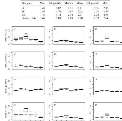
Figure 7 compares the distribution of the SOC content of the three soil sample sets to the LTFE archive data (Fig. 1). A Mann–WhitneyUtest was applied. The statistics of the data
Figure 7.Soil organic carbon (SOC) content of the three soil sam-ple sets A (left), B (middle), and all (middle) and of archive data measured from 2004 to 2007 (right). The thin line shows the 95 % confidence interval, the bar the interquartile range, and the dot the median. Mann–WhitneyUtest was used to compare A, B, and all samples to the archive data. The three soil sample sets were not compared among each other.
Table 3.Statistics of soil organic carbon in percent for the three different soil sample sets and the per-plot soil archive data.
Samples Min. 1st quartile Median Mean 3rd quartile Max.
A 1.47 1.82 2.21 2.11 2.36 2.93
B 1.49 1.70 1.97 2.02 2.31 2.74
all 1.47 1.72 2.12 2.01 2.35 2.93
Archive data 1.49 1.89 2.09 2.08 2.33 2.64
Figure 8.Boxplots of test-set RMSEMVobtained with the various datasets. Figure columns refer to datasets using(a)A samples,(b)B samples, and(c)all samples. Figure rows refer to the applied pre-processing, 1−SG, 2−SGCR, 3−SNVd1, 4−gapDer.
3.2 Comparison of datasets and pre-processing methods
Figure 8 shows the box plots of the RMSEMV. The results of the six datasets corresponding to different information con-cerning SOC values and spectra (Table 2) are displayed in one plot. The results according to the various pre-processing methods (compare Fig. 4) are displayed in figure lines 1 to 4, and the results of the models built from the data correspond-ing to A samples, B samples, and all samples are shown in figure columns a, b, and c. As 5-fold CV with five repetitions was performed, five RMSEMVtest sets are shown in each box plot.
As expected, the dataset of three SOC replicate measure-ments with one averaged spectrum (Dataset100) resulted in
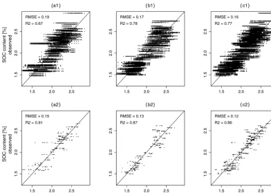
Figure 9.Comparison of predicted and observed soil organic carbon (SOC) values for Dataset111(a1toc1) and Dataset000(a2toc2) for five repetitions with the corresponding best pre-processing (SGCR for data A and all data, SG for data B);(a)shows results for A samples, (b)for B samples, and(c)for all samples. The depicted RMSE andR2values refer to the mean of five repetitions.
considered: model performance results display an increase of RMSE values from Dataset000to Dataset001to Dataset011 due to the fact that more spectral variance was related to the same target information concerning SOC. This applies to three of the four spectral pre-processing variants (SG, SGCR, gapDer), while SNVd1 pre-processing displays an unexpected pattern with datasets including replicate mea-surements and multiple scans even outperforming those with averaged data. Overall SGCR resulted in the best model per-formance for data A (Fig. 8a2) and all samples (Fig. 8c2), while SG pre-processing resulted best for data B (Fig. 8b1). However, the latter does not apply for Dataset000, where gapDer pre-processing resulted in the best model perfor-mance with RMSEMV=0.13.
The overall best pre-processing methods in this study were the combination of SG and CR as well as SG alone. SG was used successfully by many authors before for spectral pre-processing. CR was used by, for example, Viscarra Rossel et al. (2016) and Loum et al. (2016) with acceptable success. The combination of SG and CR could not be found in liter-ature, though. SNV was applied before by other authors in order to remove baseline effects (Knadel et al., 2015; Mi-nasny et al., 2011; Viscarra Rossel et al., 2006a). The pre-processing technique d1 was found to lead to poorer model results and rather unexpected performance patterns in this
study. The former may have its cause in the tendency of d1 to increase noise (Leone et al., 2012; Stevens and Ramirez Lopez, 2014). We do not have an explanation for the latter, though. Leone et al. (2012) suggested the usage of SG in combination with d1 to solve the problem. For the usage of gapDer no comparison could be found in the literature.
Comparing the mean RMSEMV, the models built on sam-ples B resulted in better model performance than those built on samples A with the exception of Dataset100. The Mann– WhitneyUtest did not show a significant difference. The A samples, as well as B samples, seem to represent the archive data in an adequate way. Nevertheless, the difference in the distribution of SOC values of A and B samples may have led to the observed different predictive capability in certain SOC value ranges. However, whether this difference is the reason for the better performance of the B models cannot be stated with certainty.
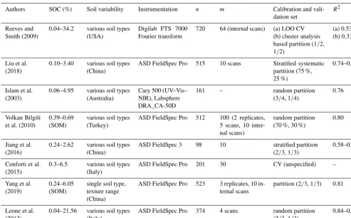
Table 4.R2model performance values from Vis–NIR applications to predict SOC.
Authors SOC (%) Soil variability Instrumentation n m Calibration and vali-dation set
R2
Reeves and Smith (2009)
0.04–34.2 various soil types (USA)
Digilab FTS 7000 Fourier transform
720 64 (internal scans) (a) LOO CV (b) cluster analysis based partition (1/2, 1/2)
(a) 0.534 (b) 0.335
Liu et al. (2018)
0.10–3.40 various soil types (China)
ASD FieldSpec Pro 515 10 scans Stratified systematic partition (75 %, 25 %)
0.74–0.83
Islam et al. (2003)
0.06–4.95 various soil types (Australia)
Cary 500 (UV–Vis– NIR), Labsphere DRA_CA-50D
161 – random partition (3/4, 1/4)
0.76
Volkan Bilgili et al. (2010)
0.39–0.69 (SOM)
various soil types (Turkey)
ASD FieldSpec Pro 512 100 (2 replicates, 5 scans, 10 inter-nal scans)
random partition (70 %, 30 %)
0.80
Jiang et al. (2016)
0.24–2.62 various soil types (China)
ASD FieldSpec 3 98 10 stratified partition (2/3, 1/3)
0.58–0.85
Conforti et al. (2015)
0.3–6.5 various soil types (Italy)
ASD FieldSpec Pro 201 30 CV (unspecified) –
Yang et al. (2019)
0.24–6.05 (SOM)
single soil type, texture range (China)
ASD FieldSpec Pro 523 3 replicates, 10 in-ternal scans
partition (2/3, 1/3) 0.81
Leone et al. (2012)
0.04–21.56 various soil types (Italy)
ASD FieldSpec Pro 374 4 scans random partition (2/3, 1/3)
0.84–0.92
n, number of samples;m, averaged spectral measurements per sample; LOO CV, leave-one-out cross-validation.
anR2of 0.77. This is further illustrated in Fig. 9 and could be expected, as Dataset000contained no input data uncertain-ties. The RMSEMVvalues, therefore, only correspond to the model building process. Overall, the best model performance which did not consider error propagation corresponded to a mean RMSEMVof 0.12 % SOC (R2=0.86). This model per-formance was impaired by1RMSEMV=0.04 % SOC while considering input data uncertainties (1R2=0.09), and by
1RMSEMV=0.12 (1R2=0.17) considering an inappro-priate pre-processing. The effect of the sampling design amounted to a 1RMSEMV of 0.02 % SOC (1R2=0.05). Overall, the additional accounting of neighbouring sample locations during fold division not only for model validation CV but also for model tuning CV might still improve the per-formance of all models. This is currently not implemented in the applied R package caret. We will, therefore, opt for other implementations in future studies.
Model performance values between studies that use Vis– NIR spectral information to predict soil properties are often compared to one another without mentioning the underly-ing range of the target variable, the variability of the mea-sured soils, the applied sampling design, measurement pro-tocol, validation approach, or applied instrumentation. Of-ten, this information is not even provided by the respective
samples for laboratory measurements. In none of the studies listed in Table 4 was the error in SOC measurements men-tioned to be considered during model building. Also, in most studies the available dataset was randomly parted into cal-ibration and validation set, using different data proportions for the two sets. Jeong et al. (2017) and Beleites et al. (2005) showed that different validation strategies led to different er-ror values. As shown in Fig. 8, the input data uncertainty had a major influence on model performance. Accordingly, the applied measurement protocol should be reported with com-plete details.
4 Conclusions
This study addressed the impact of various data and mod-elling aspects on model performance with a focus on the propagation of input data uncertainties. Overall, the best model performance which did not consider uncertainty prop-agation corresponded to a mean RMSEMV of 0.12 % SOC (R2=0.86). This model performance was impaired by
1RMSEMV=0.04 % SOC considering input data uncer-tainties (1R2=0.09) and by 1RMSEMV=0.12 % SOC (1R2=0.17) considering an inappropriate pre-processing. The effect of the sampling design amounted to a1RMSEMV of 0.02 % SOC (1R2=0.05).
Overall, the applied nestedk-fold group CV approach can be recommended in general. Furthermore, this study showed that it is of uttermost importance to clarify which informa-tion is contained in the reported error values. We, therefore, emphasize the necessity of a transparent and precise docu-mentation of the measurement protocol, the model building, and validation procedure, including the calculation of the er-ror measure, in order to assess model performance in a com-prehensive way and allow for comparison between publica-tions. Particularly, when Vis–NIR spectrometry is used for soil monitoring, the aspect of uncertainty propagation in the involved modelling procedure becomes essential.
Data availability. The data of this study are available from https://doi.org/10.17605/OSF.IO/TN4KU (Ließ, 2019).
Author contributions. ME conducted spectral lab measure-ments, data analysis, and manuscript writing. IM provided access to the LTFE site as well as corresponding information and the archive data. UW provided lab facilities and supervised the spectral mea-surements. ML was responsible for sampling setup and data acquisi-tion, conceptual embedding of the manuscript, manuscript writing, and revision during the review process.
Competing interests. The authors declare that they have no con-flict of interest.
Acknowledgements. We are grateful to the support of our col-leagues from the UFZ departments of Soil System Science, Com-munity Ecology, Monitoring and Exploration Technologies, and Computational Landscape Ecology for support during the field cam-paign and the consequent sample preparation and laboratory analy-sis.
Review statement. This paper was edited by Nikolaus J. Kuhn and reviewed by three anonymous referees.
References
Abdi, H.: Partial Least Square Regression – PLS-Regression, in: Encyclopedia of Measurement and Statistics, edited by: Salkind, N., ThousandOaks (CA), Sage., 2007.
Adamchuk, V. I. and Viscarra Rossel, R. A.: Development of On-the-Go Proximal Soil Sensor Systems, in: Proximal Soil Sens-ing. Progress in Soil Science, edited by: Viscarra Rossel, R. A., McBratney, A., and Minasny, B., 15–28, Springer, Dordrecht, 2010.
Altermann, M., Rinklebe, J., Merbach, I., Körschens, M.,
Langer, U., and Hofmann, B.: Chernozem – Soil of
the Year 2005, J. Plant Nutr. Soil Sc., 168, 725–740, https://doi.org/10.1002/jpln.200521814, 2005.
Barnes, R. J., Dhanoa, M. S., and Lister, S. J.: Standard Normal Variate Transformation and De-Trending of Near-Infrared Dif-fuse Reflectance Spectra, Appl. Spectrosc., 43, 772–777, 1989.
Beleites, C., Baumgartner, R., Bowman, C., Somorjai,
R., Steiner, G., Salzer, R., and Sowa, M. G.:
Vari-ance reduction in estimating classification error using sparse datasets, Chemometr. Intell. Lab., 79, 91–100, https://doi.org/10.1016/j.chemolab.2005.04.008, 2005.
Ben-Dor, E., Irons, J. A., and Epema, A.: Soil Spectroscopy, in: Manual of Remote Sensing, edited by: Rencz, A., 111–188, J. Wiley & Sons, Inc., NewYork, 1999.
Ben Dor, E., Ong, C., and Lau, I. C.: Reflectance measurements of soils in the laboratory: Standards and protocols, Geoderma, 245– 246, 112–124, https://doi.org/10.1016/j.geoderma.2015.01.002, 2015.
Bjørsvik, H.-R. and Martens, H.: Data Analysis: Calibration of NIR Instruments by PLS Regression, in Handbook of Near-Infrared Analysis, edited by: Burns, D. A. and Ciurczak, E. W., 189–205, 2008.
Brown, J. D. and Heuvelink, G. B. M.: Assessing Uncertainty Prop-agation through Physically Based Models of Soil Water Flow and Solute Transport, in: Encyclopedia of Hydrological Sciences, edited by: Anderson, M. G., 1181–1195, Wiley, Chicester, UK, 2006.
Charrad, M., Ghazzali, N., Boiteau, V., and Niknafs, A.: NbClust: An R Package for Determining the Relevant Number of Clusters in a Data Set, J. Stat. Softw., 61, 1–36, 2014.
Croft, H., Kuhn, N. J., and Anderson, K.: On the use of remote sensing techniques for monitoring spatio-temporal soil organic carbon dynamics in agricultural systems, Catena, 94, 64–74, https://doi.org/10.1016/j.catena.2012.01.001, 2012.
Dalal, R. C. and Henry, R. J.: Simultaneous Determination of Moisture, Organic Carbon, and Total Nitrogen by Near Infrared Reflectance Spectrophotometry1, Soil Sci. Soc. Am. J., 50, 120, https://doi.org/10.2136/sssaj1986.03615995005000010023x, 1986.
Dierke, C. and Werban, U.: Geoderma
Relation-ships between gamma-ray data and soil properties
at an agricultural test site, Geoderma, 199, 90–98,
https://doi.org/10.1016/j.geoderma.2012.10.017, 2013.
Filzmoser, P. and Gschwandtner, M.: Package “mvoutlier”: Multi-variate outlier detection based on robust methods, R package ver-sion 2.0.9, available at: https://cran.r-project.org/web/packages/ mvoutlier/mvoutlier.pdf (last access: 18 September 2019), 2018. Ge, Y., Morgan, C. L. S., Grunwald, S., Brown, D. J., and Sarkhot, D. V.: Comparison of soil reflectance spectra and calibra-tion models obtained using multiple spectrometers, Geoderma, 161, 202–211, https://doi.org/10.1016/j.geoderma.2010.12.020, 2011.
Gholizadeh, A., Boruvka, L., Sbaerioon, M., and Vasat, R.: Visible, near-infrared, and mid-infrared spectroscopy applications for soil assessment with emphasis on soil organic matter content and quality: State-of-the-art and key issues, Appl. Spectrosc., 67/12, 1349–1362, 2013.
Guio Blanco, C. M., Brito Gomez, V. M., Crespo, P., and Ließ, M.: Spatial prediction of soil water retention in a Páramo landscape: Methodological insight into machine learning using random forest, Geoderma, 316, 100–114, https://doi.org/10.1016/j.geoderma.2017.12.002, 2018.
Hastie, T., Tibshirani, R., and Friedman, J. H.: The Elements of Sta-tistical Learning, 2nd Edn., Springer, New York, 2009.
Heuvelink, G. B. M.: Propagation of error in spatial modelling with GIS, in: Geographical Information Systems, edited by: Longley, P. A., Goodchild, M. F., Maguire, D. J., and Rhind, D. W., 207– 217, New York, John Wiley & Sons, 1999.
Islam, K., Singh, B., and McBratney, A. B.: Simultaneous estima-tion of several soil properties by ultra-violet, visible, and near-infrared reflectance spectroscopy, Aust. J. Soil Res., 41, 1101– 1114, https://doi.org/10.1071/SR02137, 2003.
Jansen, M.: Prediction error through modelling concepts and un-certainty from basic data, Nutr. Cycl. Agroecosys., 50, 247–253, https://doi.org/10.1023/A:1009748529970, 1998.
Jeong, G., Choi, K., Spohn, M., Park, S. J., Huwe, B., and Ließ, M.: Environmental drivers of spatial patterns of top-soil nitrogen and phosphorus under monsoon conditions in a complex terrain of South Korea, PLoS One, 12, 1–19, https://doi.org/10.1371/journal.pone.0183205, 2017.
Jiang, Q., Chen, Y., Guo, L., Fei, T., and Qi, K.: Estimating Soil Organic Carbon of Cropland Soil at Different Levels of Soil Moisture Using VIS-NIR Spectroscopy, Remote Sens., 8, 755, https://doi.org/10.3390/rs8090755, 2016.
Johnson, M. G.: Soil carbon sequestration: Quantifying this ecosys-tem service, Present. Oregon Soc. Soil Sci. Annu. Meet., 28– 29 February 2008, Newport, OR, 2008.
Kennard, R. W. and Stone, L. A.: Computer Aided Design of Ex-periment, Technometrics, 11, 137–148, 1969.
Knadel, M., Thomsen, A., Schelde, K., and Greve, M. H.: Soil organic carbon and particle sizes mapping using vis-NIR, EC and temperature mobile sensor platform, Comput. Electron. Agr., 114, 134–144, https://doi.org/10.1016/j.compag.2015.03.013, 2015.
Körschens, M. and Pfefferkorn, A.: Bad Lauchstädt – The Static Fertilization Experiment and other Long-Term Field Experi-ments, UFZ – Umweltforschungszentrum Leipzig-Halle GmbH, 1998.
Kuang, B. and Mouazen, A. M.: Non-biased prediction of soil or-ganic carbon and total nitrogen with vis e NIR spectroscopy, as affected by soil moisture content and texture, Biosyst. Eng., 114, 249–258, https://doi.org/10.1016/j.biosystemseng.2013.01.005, 2013.
Kuhn, M.: Package “caret”: Classification and regression train-ing, Version 6.0-84, available at: https://cran.r-project.org/web/ packages/caret/caret.pdf (last access: 18 September 2019), 2017. Kuhn, M. and Johnson, K.: Applied Predictive Modeling, Springer,
New York Heidelberg Dordrecht London, 2013.
Lal, R.: Soil Carbon Sequestration Impacts on Global Cli-mate Change and Food Security, Science, 304, 1623–1627, https://doi.org/10.1126/science.1097396, 2004.
Lê, S., Josse, J., and Husson, F.: FactoMineR: An R Pack-age for Multivariate Analysis, J. Stat. Softw., 25, 1–18, https://doi.org/10.1016/j.envint.2008.06.007, 2008.
Leone, A. P., Viscarra Rossel, R. A., Amenta, P., and Buondonno, A.: Prediction of Soil Properties with PLSR and vis-NIR Spectroscopy?: Application to Mediterranean Soils from Southern Italy, Curr. Anal. Chem., 8, 283–299, https://doi.org/10.2174/157341112800392571, 2012.
Ließ, M.: DATA: Error propagation in
spectromet-ric functions of soil organic carbon, OSF Home,
https://doi.org/10.17605/OSF.IO/TN4KU, 2019.
Liu, Y., Zhou, S., Zhang, G., Chen, Y., Li, S., Hong, Y., Shi, T., Wang, J., and Liu, Y.: Application of spectrally derived soil type as ancillary data to improve the estimation of soil organic car-bon by using the Chinease soil Vis-NIR spectral library, Remote Sens., 10, 1–16, https://doi.org/10.3390/rs10111747, 2018. Lorenz, K. and Lal, R.: Soil Organic Carbon – An Appropriate
In-dicator to Monitor Trends of Land and Soil Degradation within the SDG Framework?, edited by: Starke, S. M. and Ehlers, K., Umweltbundesamt, Dessau-Roßlau„ 2016.
Loum, M., Diack, M., Ndour, N. Y. B., and Masse, D.: Effect of the Continuum Removal in Predicting Soil Or-ganic Carbon with Near Infrared Spectroscopy (NIRS) in the Senegal Sahelian Soils, Open J. Soil Sci., 6, 135–148, https://doi.org/10.4236/ojss.2016.69014, 2016.
Martens, H. and Næs, T.: Multivariate Calibration, JohnWiley & Sons, Chichester, UK, 1989.
McBratney, A. B., Stockmann, U., Angers, D. A., Minasny, B., and Field, D. J.: Challenges for Soil Organic Carbon Research, in Soil Carbon, Progress in Soil Science, edited by: Hartemink, A. E. and McSweeney, K., p. 57, Springer International Publishing, Switzerland, 2014.
Merbach, I. and Schulz, E.: Long-term fertilization effects on crop yields, soil fertility and sustainability in the Static Fer-tilization Experiment Bad Lauchstädt under climatic condi-tions 2001–2010, Arch. Agron. Soil Sci., 59, 1041–1057, https://doi.org/10.1080/03650340.2012.702895, 2013.
Minasny, B., McBratney, A. B., Bellon-Maurel, V., Roger, J.-M., Gobrecht, A., Ferrand, L., and Joalland, S.: Removing the ef-fect of soil moisture from NIR diffuse reflectance spectra for the prediction of soil organic carbon, Geoderma, 167–168, 118–124, https://doi.org/10.1016/j.geoderma.2011.09.008, 2011.
Molinaro, A. M., Simon, R., and Pfeiffer, R. M.: Prediction error es-timation: a comparison of resampling methods, Bioinformatics, 21, 3301–3307, 2005.
Mortensen, P.: Myth: A partial least squares calibration model can never be more precise than the reference method. . . , NIR News, 25, 20–22, 2014.
Mouazen, A. M., Kuang, B., De Baerdemaeker, J., and Ramon, H.: Comparison among principal component , partial least squares and back propagation neural network analyses for ac-curacy of measurement of selected soil properties with vis-ible and near infrared spectroscopy, Geoderma, 158, 23–31, https://doi.org/10.1016/j.geoderma.2010.03.001, 2010.
Naes, T., IsakssonT., Fearn, T., and Davies, T.: A User Friendly Guide to Multivariate Calibration and Classification, NIR Pub-lications, Chichester, 2002.
Nieder, R. and Benbi, D. K.: Carbon and Nitrogen in the Terrestrial Environment, Springer, the Netherlands, 2008.
Nduwamungu, C., Ziadi, N., Parent, L.-E., Tremblay, G. F., and Thuriès, T.: Opportunities for, and Limitations of, Near Infrared Reflectance Spectroscopy Applications in Soil Analysis: A Re-view, Can. J. Soil Sci., 89, 531–541, 2009.
Nocita, M., Stevens, A., Noon, C., and Van Wesemael, B.: Pre-diction of soil organic carbon for different levels of soil moisture using Vis-NIR spectroscopy, Geoderma, 199, 37–42, https://doi.org/10.1016/j.geoderma.2012.07.020, 2013.
Pilorget, C., Fernando, J., Ehlmann B., Schmidt, F., and Hiroi, T.: Wavelength dependence of scattering properties in the VIS–NIR and links with grain-scale physical and compositional properties, Icarus, 267, 296–314, 2016.
Pimstein, A., Notesco, G., and Ben-Dor, E.: Performance of Three Identical Spectrometers in Retrieving Soil Reflectance under Laboratory Conditions, Soil Sci. Soc. Am. J., 75, 746, https://doi.org/10.2136/sssaj2010.0174, 2011.
Poggio, L. and Gimona, A.: National scale 3D modelling of soil or-ganic carbon stocks with uncertainty propagation – An example from Scotland, Geoderma, 232–234, 284–299, 2014.
Reeves, J. B. and Smith, D. B.: The potential of mid- and near-infrared diffuse reflectance spectroscopy for determining major-and trace-element concentrations in soils from a geochemical survey of North America, Appl. Geochem., 24, 1472–1481, https://doi.org/10.1016/j.apgeochem.2009.04.017, 2009. Rinnan, Å., van den Berg, F., and Engelsen, S. B.: Review
of the most common pre-processing techniques for near-infrared spectra, TrAC – Trend Anal. Chem., 28, 1201–1222, https://doi.org/10.1016/j.trac.2009.07.007, 2009.
Savitzky, A. and Golay, M. J. E.: Smoothing and Differentiation of Data by Simplified Least Squares Procedures, Anal. Chem., 36, 1627–1639, https://doi.org/10.1021/ac60214a047, 1964.
Schulz, E.: Static Fertilization Experiment Bad Lauchstädt, avail-able at: http://www.ufz.de/index.php?en=37010 (last access: Oc-tober 2018), 2017.
Schwartz, G., Eshel, G., and Ben-Dor, E.: Reflectance Spectroscopy as a Tool for Monitoring Contaminated Soils, in: Soil Con-tamination, edited by: Pascucci, S., InTech, New York, 67–90, https://doi.org/10.5772/23661, 2011.
Stenberg, B. and Viscarra Rossel, R. A.: Diffuse Reflectance Spec-troscopy for High-Resolution Soil Sensing, in: Proximal Soil Sensing. Progress in Soil Science, edited by: Viscarra Rossel, R. A., McBratney, A., and Minasny, B., 29–47, Springer, Dordrecht, 2010.
Stenberg, B., Viscarra Rossel, R. A., Mouazen, A. M., and Wet-terlind, J.: Visible and Near Infrared Spectroscopy in Soil Sci-ence, Adv. Agron., 107, 163–215, https://doi.org/10.1016/s0065-2113(10)07005-7, 2010.
Stevens, A. and Ramirez Lopez, L.: An introduction to the prospectr package, 1–22, available at: http://cran.r-project.org/ web/packages/prospectr/vignettes/prospectr-intro.pdf (last ac-cess: November 2018), 2014.
Stevens, A., Nocita, M., Tóth, G., Montanarella, L., and
van Wesemael, B.: Prediction of Soil Organic
Car-bon at the European Scale by Visible and Near In-fraRed Reflectance Spectroscopy, PLoS One, 8, e66409, https://doi.org/10.1371/journal.pone.0066409, 2013.
Stockmann, U., Adams, M. A., Crawford, J. W., Field, D. J., Henakaarchchi, N., Jenkins, M., Minasny, B., Mcbratney, A. B., Remy, V. De, Courcelles, D., Singh, K., Wheeler, I., Abbott, L., Angers, D. A., Baldock, J., Summers, D., Lewis, M., Ostendorf, B., and Chittleborough, D.: Visible near-infrared reflectance spectroscopy as a predictive indicator of soil properties, Ecol. In-dic., 11, 123–131, https://doi.org/10.1016/j.ecolind.2009.05.001, 2011.
Varma, S. and Simon, R.: Bias in error estimation when using cross-validation for model selection, BMC Bioinformatics, 7, 91, https://doi.org/10.1186/1471-2105-7-91, 2006.
VDLUFA: Methodenbuch Band I Die Untersuchung von Böden, in: Das VDLUFA Methodenbuch, VDLUFA-Verlag, Darmstadt, 2012.
Viscarra Rossel, R. A., Walter, C., and Fouad, Y.: Assessment of two reflectance techniques for the quantification of the within-field spatial variability of soil organic carbon, edited by: Stafford, J. and Werner, A., Precision Agriculture. Fourth European Con-ference on Precsision Agriculture, Wageningen Academic Pub-lishers, Berlin, 697–702, 2003.
Viscarra Rossel, R. A., McGlynn, R. N., and McBratney, A. B.: De-termining the composition of mineral-organic mixes using UV-vis-NIR diffuse reflectance spectroscopy, Geoderma, 137, 70–82, https://doi.org/10.1016/j.geoderma.2006.07.004, 2006a. Viscarra Rossel, R. A., Walvoort, D. J. J., McBratney, A. B., Janik,
L. J., and Skjemstad, J. O.: Visible, near infrared, mid infrared or combined diffuse reflectance spectroscopy for simultaneous assessment of various soil properties, Geoderma, 131, 59–75, https://doi.org/10.1016/j.geoderma.2005.03.007, 2006b. Viscarra Rossel, R. A., Behrens, T., Ben-Dor, E., Brown, D. J.,
C., Grunwald, S., Gubler, A., Guerrero, C., Hedley, C. B., Knadel, M., Morrás, H. J. M., Nocita, M., Ramirez-Lopez, L., Roudier, P., Campos, E. M. R., Sanborn, P., Sellitto, V. M., Sudduth, K. A., Rawlins, B. G., Walter, C., Winowiecki, L. A., Hong, S. Y., and Ji, W.: A global spectral library to characterize the world’s soil, Earth-Sci. Rev., 155, 198–230, https://doi.org/10.1016/j.earscirev.2016.01.012, 2016.
Volkan Bilgili, A., van Es, H. M., Akbas, F., Durak, A., and Hively, W. D.: Visible-near infrared reflectance spec-troscopy for assessment of soil properties in a
semi-arid area of Turkey, J. Arid Environ., 74, 229–238,
https://doi.org/10.1016/j.jaridenv.2009.08.011, 2010.
Wang, Y., Lu, C., Wang, L., Song, L., Wang, R., and Ge, Y.: Predic-tion of Soil Organic Matter Content Using VIS/NIR Soil Sensor, Sensors & Transducers, 168, 113–119, 2014.
Wehrens, R.: Chemometrics with R – Multivariate Data Analysis in the Natural Sciences and Life Sciences, edited by: Gentleman, G. P. R. and Hornik, K., Springer-Verlag Berlin Heidelberg, 2011. Yang, M., Xu, D., Chen, S., Li, H., and Shi, Z.: