A Machine Learning Approach to Study the
Relationship between Features of the Urban
Environment and Street Value
Alessandro Venerandi1,*,† , Giovanni Fusco1,† , Andrea Tettamanzi2,‡ and David Emsellem3,§
1 ESPACE, CNRS, Université Côte d’Azur, 06200 Nice, France; [email protected] 2 I3S, Inria, CNRS, Université Côte d’Azur, 06900 Sophia Antipolis, France;
3 KCITYLABS (Kinaxia Group), 06560 Valbonne, France; [email protected]
* Correspondence: [email protected] † Current address: 98, Bd Herriot, BP 3209, 06200 Nice, France.
‡ Current address: 2000, route des Lucioles, 06900 Sophia Antipolis, France. § Current address: 80, route des Lucioles, 06560 Valbonne, France.
Received: 17 July 2019; Accepted: 10 September 2019; Published: 14 September 2019
Abstract: Understanding what aspects of the urban environment are associated with better socioeconomic/liveability outcomes is a long standing research topic. Several quantitative studies have investigated such relationships. However, most of such works analysed single correlations, thus failing to obtain a more complete picture of how the urban environment can contribute to explain the observed phenomena. More recently, multivariate models have been suggested. However, they use a limited set of metrics, propose a coarse spatial unit of analysis, and assume linearity and independence among regressors. In this paper, we propose a quantitative methodology to study the relationship between a more comprehensive set of metrics of the urban environment and the valorisation of street segments that handles non-linearity and possible interactions among variables, through the use of Machine Learning (ML). The proposed methodology was tested on the French Riviera and outputs show a moderate predictive capacity (i.e., adjustedR2=0.75) and insightful
explanations on the nuanced relationships between selected features of the urban environment and street values. These findings are clearly location specific; however, the methodology is replicable and can thus inspire future research of this kind in different geographic contexts.
Keywords:urban environment; street value; machine learning; ensemble method; French Riviera
1. Introduction
Since the advent of Geographic Information Systems (GIS), several researchers have quantitatively investigated the relationship between aspects of the urban environment and various liveability and socioeconomic outputs, in particular in the fields of urban design and urban morphology. For example, Vaughan et al. analysed the relationship between street network accessibility and socioeconomic levels in East London and found that more segregated streets were associated with more disadvantaged social classes [1]. Hillier studied whether dead-end roads were related to more or less crimes in a London neighbourhood and found that they were not associated with more criminal activity, if the surrounding streets were characterised by through passage and buildings abutting on them [2]. Urban crimes have also been studied in relation to density. While Harries did not find a significant relationship [3], other researchers found that more density was associated with less reported crimes [4]. Other researchers analysed density in relation to social aspects. While Duany et al. found that the former was associated with better social ties [5], Burchell et al. reported that lower densities not only diminished social
interactions, but also favoured car use [6]. Such studies clearly provide relevant empirical results on the relationships between single urban features and different socioeconomic aspects. However, the urban environment is a much more complex entity, characterised by multiple factors that act together rather than in isolation [7,8]. More recently, a methodology to study socioeconomic indexes that accounted for multiple urban features and utilised multivariate spatial regression rather than correlation has been proposed [9]. It was tested on six UK cities and showed that more population density, unbuilt land, and dead-end roads, as well as a more regular street layout were associated with more socioeconomically deprived neighbourhoods. However, the methodology proposed only nine metrics, which is certainly an improvement over previous works, but, we argue, they are not enough to obtain a comprehensive picture of the urban realm. Furthermore, the use of linear models implies linearity and independence among regressors. These two conditions are hardly met considering that the phenomena under exam might not behave in a linear fashion. For example, if we consider socioeconomic deprivation, it might well be that areas near major infrastructures are more deprived. However, this relationship might decay faster than in a linear manner in areas located further away. Secondly, variables measuring spatial phenomena in the same study area tend to be correlated, thus violating the assumption of independence of observations. Thirdly, it was suggested to use areas as spatial units of analysis, although street segments (i.e., the line connecting two street intersections), in our view, might be a better choice, especially when analysing configurational and morphological aspects of cities.
The phenomenon investigated in this paper is place value—or at least one of its aspects—as more widely discussed by Carmona [10]. More precisely, we aimed at explaining the geography of place value of each street segment, in any large metropolitan area, as it emerges from housing transactions (i.e., street value). Without denying the interest in other facets of social valorisation of urban space (e.g., symbolic and cultural valorisation), we used housing prices as a practical thermometer to gauge a fairly comparable social value, granted by households and urban actors in different city areas. Explaining the spatial distribution of street value using metrics of the urban environment is a challenging task for which no unified theoretical approach exists. Natural movement theory [11], urban morphology approaches [8], human ecology and its subsequent reinterpretations by urban geography [12] propose different and concurrent theoretical frameworks. Together with the aforementioned methodological issues, this justifies more exploratory approaches in high-dimensional databases of metrics of the urban environment, which can today be investigated through ML.
In this paper, we thus propose an ensemble method based on ML—and thus able to handle non-linearity and interactions among regressors—to analyse the relationship between a comprehensive set of features of the urban environment and street value. More specifically, such method: (i) computes a metric of residential valorisation at the street level (i.e., street value), through the aggregation of housing transactions; (ii) provides instructions on how to characterise the urban environment of any study area in the most comprehensive way possible; (iii) applies a ML feature selection algorithm to select the best descriptors for the study area under exam; (iv) implements Gradient Boosting (GB) to model the relationships between street value and the selected variables; (v) tests residuals for spatial autocorrelation, whose presence is sign of model under-specification; and (vi) uses a recently developed algorithm to render the outcomes of the GB model human-interpretable. Such methodology was tested on the French Riviera to study the relationship between street values, obtained from around 110,000 housing transactions exchanged in the period 2008–2017, and more than 100 metrics quantifying different aspects of the urban environment, including configurational, morphological, and natural features. Outcomes of such analysis show a moderately high predictive capacity (i.e., adjusted
effect with distance to rail track. Being at easy reach to the coast but, at the same time, close to rail tracks depresses street values.
The use of housing transaction data echoes a well-developed line of research in econometrics, i.e., the explanation of housing price formation through hedonic modelling [13]. These models traditionally rely on a set of intrinsic (e.g., habitable surface, number of bedrooms, and presence of a garden and other elements of comfort) and extrinsic features (e.g., proximity to the closest underground station and accessibility to services and amenities) to explain house prices. They are also increasingly integrating place-based effects through multi-level approaches [14,15] and the combination of spatial (e.g., geographically weighted regression) and repeat sales models [16]. More recently, ML techniques have also been adopted, for example, to correct spatial errors in predictions of repeat sales models [17] and to improve the aggregation of spatial effects in econometric models [18]. Our aim is however different. We are not interested in the prediction of prices per se or in discovering the monetary contribution of each of the features used in the model. Our focus is understanding the subtleties of the relationship between a set of relevant features of the urban environment and the valorisation of fragments of urban space (i.e., street segments) widely recognised as fundamental spatial units for the study of urban phenomena [11,19,20].
We argue that the ensemble method proposed in this paper might help researchers in the fields of urban geography, urban morphology, and urban design who are interested in exploring the nuanced relationships existing between locally relevant features of the urban environment and street value. The methodology can also be used for comparative analysis and thus to test whether or not specific relationships hold in different geographic contexts. Finally, it contributes to an emerging need in the study of social systems (i.e., coupling predictive accuracy and interpretability of outcomes) [21].
The remainder of this paper is structured as follows. In the next section, we provide details on the methodology proposed, including the metrics of street value, metrics of the urban environment and the ensemble of ML techniques to model the relationship between them. We then follow by illustrating the empirical application of the proposed method to the French Riviera. This part includes a presentation of the data sources used to compute the metrics, the empirical outputs and their interpretations. Finally, we conclude with limitations, future work, and final remarks.
2. Methodology
In this section, we present, firstly, the spatial unit of analysis adopted; secondly, we illustrate how to compute the metric of street value by aggregating housing transactions for street segments; thirdly, we suggest what aspects of the urban environment to consider for calculating metrics; finally, we provide details on the proposed ensemble of ML techniques to model the relationship between the metrics previously calculated.
2.1. Spatial Unit of Analysis
2.2. Street Value
This step assumes that the housing transactions to be analysed are in data point format. To compute the metric of residential valorisation at the street level, it is necessary to, firstly, process the data on housing transactions to render values comparable across different years and housing types and, secondly, to compute a measure of central tendency from such processed dataset. We illustrate these two steps next.
2.2.1. Pre-Processing
Housing transactions of different years and housing typologies cannot be directly compared due to yearly inflation, housing market cycles (e.g., economic recession or upturn), and specific market behaviours affecting different housing types. For example, bigger properties tend to be sold less frequently as they are more expensive and are thus long-term investments, while smaller properties, due to their relatively lower values, tend to be exchanged more easily and tend to be short-term investments. The average price per square metre tends also to be structurally higher for small flats for technical reasons (even the smallest flat needs sanitary and cooking equipment, which proportionally weigh more on the average price per surface unit compared to a larger property). The very notion of average price per square metre can thus be challenged when applied to such diverse housing markets. To address these issues, instead of the conventional price per square metre, our method requires to separate the transactions by year and housing type and compute ventiles of prices for each subset year of transaction and housing type. We consider such statistic an appropriate normalised value, which account for different market segments and years, thus making transactions comparable among them.
2.2.2. Computation of Median of Values
Having classified each transaction in a ventile of value, the next step requires to, firstly, assign to each data point the street segment to which they belong and, secondly, aggregate the information on value at the street level through the computation of a measure of central tendency (i.e., median). Such measure provides information on the central point of the distribution of housing values, in each spatial unit. We suggest performing such computation for the ensemble of each street segment and its immediate neighbouring streets, with at least 10 transactions, for three reasons: firstly, transactions located in streets directly connected to one another tend to have similar valuations (due to the influence of the same locational factors, presence of properties at the intersection of streets segments, etc.); secondly, data on house prices tend to be quite sparse, even for several years, and thus a local interpolation would allow having more streets covered with data; and, thirdly, we want to assure the reliability of the median statistics.
2.3. Metrics of the Urban Environment
cities. Finally, the accessibility to amenities and proximity to nuisances (e.g., noisy and polluting infrastructures) are further known factors that influence values. See, for example, the works by Bartholomew and Ewing [29] and Brainard et al. [30]. Next, we present possible metrics derived from these studies, categorised in three main urban subsystems: settlement system, infrastructural system, and environmental system. Note that the aim of this section is not to provide a fixed list of metrics, but rather to offer guidance on what aspects to measure. It is then up to the researcher to choose the best list of descriptors for her study area.
2.3.1. Settlement System
Urban Fabric
The urban fabric is the set of relations between buildings, streets, parcels and open space at the scale of a small urban fragment. Modern European cities are characterised by the presence of different types of urban fabrics; for example, there exist a dense and irregular one, typical of historic centres, a more spaced out and regular one, common to urban extensions of the XIX and early XX century, and a more discontinuous one, characterised by free-standing buildings surrounded by lawns and parking lots, typical of the modernist period. Quantitative measures of the forms of urban fabrics can be found, for example, in the works by Berghauser-Pont and Haupt [31], Gil et al. [32], Araldi and Fusco [33], and Venerandi et al. [34]. For example, Araldi and Fusco proposed the Multiple Fabric Assessment method (MFA), a technique that automatically detects types of urban fabrics based on morphometric descriptors of proximity bands around street segments, by taking into account the contextual role of interconnected street segments.
Configuration of the Street Network
The configuration of the street network concerns the way streets are arranged, the extent to which they are inter-connected among one another, and their relative importance for the functioning of the overall network. Configurational analyses can be used to characterise the positional characteristics of street segments at different scales (e.g., the whole city, a given neighbourhood around a specific street). Metrics to quantify such aspects are, for example, betweenness and closeness centrality [19]. The former is based on the concept that central means to be used by many of the shortest paths linking couples of street intersections in a street network. The latter measures centrality as a function of distance and thus street segments that are connected and lie at short distance between one another will have higher values of closeness. These two are not the only centrality measures that one can use, but they are the ones that were more widely adopted and for which there exist more robust scientific findings. See, for example, the works by Porta et al. in Parma (Italy) [35], Baton Rouge (LA, US) [36], and Barcelona (Spain) [37].
Functions
values. Fusco et al. utilised this very same approach to compute a measure of density of retailers in Nice, France [39].
Housing Stock
Housing stock refers to the status of the properties in each street segment, for example, their build periods or whether they are occupied as main or second homes, or whether they are vacant or not. These aspects can be quantified, for example, by calculating the proportion of properties with any special status with respect to the total number of properties present in a street. A further aspect that might affect valuations and that should thus be eventually considered is the presence of social housing. This can be quantified, for example, through the NetKDE technique mentioned in the paragraph above, whose output would consist of hotspot of social housing at the street level.
2.3.2. Infrastructural System
Public Transport Hubs
Public transport hubs are the exchange nodes in the public transport network and can be, for example, bus stops, tram stops, and train stations. The same density computation technique (i.e., NetKDE) presented in the paragraph Functions can be adopted in this case to obtain density measures of public transport hubs on the street network.
Nuisances
Nuisances in cities are usually due to noise and pollution and tend to be associated with the presence/proximity to large infrastructures, such as major roads/intersections and main transport hubs (e.g., airports and main train stations). Since noise and pollution tend to spread through air, we argue that metrics of nuisances can be computed as Euclidean distances from the midpoints of each street segment to the sources of such nuisances.
2.3.3. Environmental System
Green/Blue Infrastructures and Landforms
With the term green/blue infrastructures, we refer not only to the natural features surrounding each street segment or accessible from it (e.g., water bodies and urban forests), but also to the form of its physical site (e.g., valley, ridge, and plateau). The former can be measured, for example, by simply calculating the distance from the midpoint of a street to its nearest landscape feature or by computing the distance covered by the shortest path that connects a street midpoint to the nearest landscape feature, along the street network. The shapes of the landscape (i.e., landforms) can be classified through specific algorithms that interpret changes and patterns in altitude in a Digital Elevation Model (DEM) and also include differences in land orientation (for matter of lighting, a north facing flank does not have the same potential impact on values than a south facing one). For classification techniques of landforms, see, for example, the work by Tagil and Jenness [40].
2.4. Ensemble Method
of the GB model human-comprehensible. We provide more details for each step next. Note that the words estimator and feature are used interchangeably in the remainder of this paper.
2.4.1. Sequential Forward Selection
In the absence of a well-established theory of the residential valorisation of urban streets, the aspects of the urban environment that one can hypothetically compute are numerous. This can potentially pose several issues at the modelling stage, for example, large computational time and data redundancy which, in turn, might add noise and ultimately lead to overfitting. To overcome these issues, we thus propose utilising the Sequential Forward Selection (SFS) technique developed by Raschka [41]. This specific type of feature selection adds one feature at the time based on a regressor performance until an optimal subset of features of the desired size is reached. In the context of this paper, the target feature would be our metric of street value, while the recursively tested features would be the metrics of the urban environment. The approach is thus both theory-driven (even if only weak theoretical assumptions are used when identifying suitable metrics of the urban environment) and data-driven (through the SFS and subsequent GB protocol). Since the modelling part of the method hereby proposed is based on GB (details on its functioning are provided in the next section), we suggest using the same kind of regressor for performance evaluation at this stage. Furthermore, to obtain a statistically robust selection, it is crucial to utilise training and testing subsets. Firstly, the algorithm should be trained on a random subset of the whole dataset. Secondly, its performance should be evaluated on the portion of dataset that has not been used. To further increase the robustness of the result,k-fold cross validation should also be implemented. This consists in splitting the dataset intok
folds, using each foldk−1 times as training set and once as testing set to be predicted. The SFS final output is a set of very significant metrics ready to be input in the GB model.
2.4.2. Modelling
To model the relationship between the metrics of the urban environment selected by the SFS technique and our measure of street value, we propose to use GB, a very versatile and robust type of non-parametric ML technique, which can be used both for classification and regression purposes [42]. The basic approach underlying GB relies on the combination of several relatively weak simple models to obtain a stronger ensemble prediction. Other ML algorithms, for example, Random Forests (RF), are based on the same concept. However, while the RF prediction is based on a simple average of the outputs of such base models, GB iteratively fits new decision tree models to output a more accurate prediction of the response variable. At each specific iteration, a new base-learner is trained based on the error of the previous iteration. The minimisation of such error is based on a functional gradient descent that optimises a loss cost function pointing in the negative gradient direction. The definition of this loss function can be arbitrary chosen. If the purpose is regression, the error function should be the classic squared-error loss. A decision tree approach (more precisely, a refined nested sequence of decision trees) offers clear advantages over linear models as it accounts for non-linear and non-monotonic relations between the target variable and the possible regressors, and for interactions among them (i.e., a threshold rule for regressor A only applies when regressor B is above or below another given threshold).
a maximum depth decreases the risk of overfitting; and to obtain higher resolution predictions, a minimum number of leaves should be used, which could also lead to overfitting. To set these hyperparameters, we suggest using a trial and error approach and inspection of learning curves, a useful tool to visualise validation and training scores for a ML model, for varying numbers of training samples. The best-case scenario, for regression purposes, has it that the curves of validation and training scores should converge to an error as close as possible to 0. This corresponds to a small variance and means that the tested model generalises well the phenomenon under exam. Usually, the most common exploratory outputs in applied research are attributable to two main scenarios: the two curves converge (i.e., low variance) but the error stays relatively high or the two curves show a significant gap (i.e., high variance), with a small error on the side of the training curve. The former scenario is synonym of poor fit and generalisation, that is no matter the amount of information we feed, the model does not represent well the underlying relationship and has high systematic errors. The latter scenario has a high variance that can eventually be reduced, for example, by adding more training instances or reducing the number of features.
Having set the GB hyperparameters through a trial and error process involving the visual inspection of learning curves, the last step consists in the performance evaluation of the fitted GB model. This can be carried out through the computation of the root mean squared error and adjusted
R2. The former indicates the average error that the model is making in predicting the response variable.
Note that such error is measured in median of ventiles, considered as cardinal values. The latter represents the amount of variance in the response variable that is predicted from the variables used in the model.
2.4.3. Testing for Spatial Autocorrelation
2.4.4. Interpretation Tool
As mentioned above, the performance of a GB model can be evaluated through root mean squared error and adjustedR2. However, these values do not provide any information on the behaviours
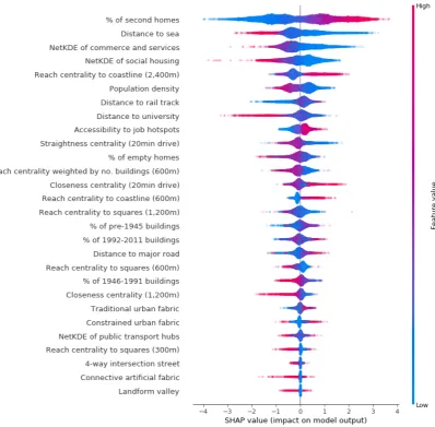
of the variables used in the model, while, from an urban geography perspective, interpreting such behaviours is of paramount importance. To contravene this, we propose the use of SHAP, a recently developed algorithm that assigns to each feature an importance value for a local prediction [46,47]. Such algorithm belongs to the class of additive feature attribution methods, a set of techniques that explain a specific prediction from a model by choosing interpretable features sampling, and then build a linear model for the local region around that prediction. However, unlike other methods, SHAP is the only one that simultaneously satisfies three properties (i.e., local accuracy, missingness, and consistency) that guarantee the quality of local approximations. The algorithm by Lundberg and Lee is able not only to provide local predictions with relative feature importance, but also—and most importantly for the scope of our work—to compute such values for the entire dataset and then summarise such information in dependence plots and a summary plot [47]. The former shows the effects that a single feature has on model outcomes and its level of interaction with another feature, which is automatically chosen by the algorithm. The latter provides an overview of the importance of all the features used in the model and also the range of their effects (positive and negative). Both dependence plots and a summary plot are crucial to understand and interpret the effects that each feature (i.e., each of the metrics of the urban environment) has on the target variable (i.e., the residential valorisation at the street level).
3. Application to the French Riviera
This section presents the results of the application of the proposed methodology to the street values, obtained from the aggregation of the housing transactions exchanged in the period 2008–2017, in the French Riviera. This section is structured as follows: firstly, we briefly introduce the study area; secondly, we illustrate the datasets from which we extracted our metrics; thirdly, we present the street values (our target variable) in the French Riviera and the metrics of the urban environment considered (our estimators); and, finally, we illustrate and interpret the outcomes of the ensemble method proposed.
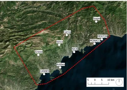
3.1. The French Riviera
Figure 1.Extents of the study area.
3.2. Datasets
To compute the metrics of street value and the urban environment for the selected study area, we accessed five different data sources: PERVAL, the French registry of housing transactions; BD TOPO, the French GIS dataset of geographic features, in vector format; census data and SIRENE, for the housing stock and urban functions; an openly accessible web platform and OpenStreetMap (OSM), for public transport data; and an official DEM, for information on the physical conformation of the area under exam. Next, we present each data source in more detail.
3.2.1. Perval
the same time period, wase475,589. In Table1, we provide more details on number of transactions and median prices, for each year.
Table 1.Number of transactions and median price for flats and single houses, for each year.
Year Flats Single Houses
No. Transactions Median Price No. Transactions Median Price
2008 - - 1858 e500,000
2009 - - 1457 e450,000
2010 13,483 e189,742 1813 e450,000
2011 14,028 e195,001 1912 e483,425
2012 11,981 e190,000 1831 e466,000
2013 12,065 e190,000 1897 e455,900
2014 12,143 e185,000 1904 e455,050
2015 12,793 e184,550 2200 e445,000
2016 10,431 e188,120 1717 e445,000
2017 9914 e190,000 1703 e445,000
3.2.2. BD TOPO
BD TOPO [49] is an official GIS database, freely accessible for research purposes, that provides vector data on various geographic entities, such us, roads, buildings, and natural features. It is issued and kept updated by IGN (the French National Institute of Geography and Forestry). BD TOPO is constituted by several datasets, one for each type of geographic entity. For the purpose of this analysis, we focused on the one containing the street network of the area under exam. This specific dataset not only had georeferenced representations of street segments, but also information on further aspects, such as street width, category (e.g., highway, regional road, local street), and travel directions. BD TOPO data are also necessary to identify and characterise urban fabrics through the MFA protocol previously mentioned [33]. The street dataset of the French Riviera utilised in this analysis dates back to March 2016 and consists of 98,297 street segments, with a median length of 78 m and a total length of 12,872 km.
3.2.3. Census Data and Sirene
In France, the French National Institute of Statistics and Economic Studies (INSEE) produces both census data and SIRENE, a dataset of commercial establishments and services. SIRENE [50] is monthly updated by INSEE and is freely accessible on the open portal of the French government. It covers the entirety of France and provides information on many aspects of commercial establishments, for example, name and surname of the owner, geographic coordinates, opening date, and category. The latter is based on a detailed taxonomy created by INSEE, which consists of several nested categories. For the purpose of this analysis, we focused on the meso-categoriesCommerce de détail(retail) and
the one used in this work. In the 426 census areas of the French Riviera, there are a total of 712,778 properties, 492,050 of which are main residences, 159,678 are second homes, and 61,050 are vacant.
3.2.4. Public Transport Data
We relied on two sources for obtaining information on public transport hubs for the area under exam: OpenMobilityData [52], a web platform that collects and makes available for download open-source public transit data from around the world, and OSM [53], probably the most renown open platform for geographic crowd-sourcing. The former provided public transit data for the network Lignes d’Azur, the transport company that serves the metropolitan region of Nice. Such data consist of georeferenced points indicating public transport hubs, such as bus stops and stations, and means of transport (e.g., bus and tram). We obtained a total of 2691 public transport hubs for the city of Nice. To fully cover the study area, we integrated this information with OSM data. This was extracted from Geofabrik [54], a website that periodically collects, organises, and makes available for download OSM data, in shapefile format, for regions and sub-regions of the world. The number of public transport hubs collected from Geofabrik, outside the city of Nice, was 1216. Thus, the total number of such hubs for the entirety of the study area was 3907. OpenMobilityData and OSM data were both accessed and downloaded in August 2018.
3.2.5. Digital Elevation Model
Information on the landforms of the French Riviera was obtained from the official DEM of the Département Alpes-Maritimes (Department of the Maritime Alps). Such DEM is issued by Aérodata France, a company specialised in the production of cartographic data through aerial photography, and comes in raster format, at a resolution of 5 m. An estimated altitude with respect to the sea level is assigned to each of the pixels of the DEM. For the study area under exam, such value ranged between 0 and 1331 m. The DEM used in this work dates back to 2009.
3.3. Metrics
3.3.1. Street Value
After having obtained PERVAL data for the portion of French Riviera under exam, we firstly performed a filtering and then applied the pre-processing presented above, before computing classes of housing values at the street level. Firstly, we filtered out those transactions that could have biased the analysis, that is properties with special contractual agreements (e.g., retirement homes), and those that did not have sufficient spatial accuracy (e.g., those geocoded at the municipal level). Secondly, since PERVAL does not provide housing types (an information required by our methodology), we created such types by combining the broad categorisation provided by PERVAL (i.e., flat or single house) with the number of rooms. By doing so, we ended up with seven housing types:
• T1 for studios and one-room flats; • T2 for two-room flats;
• T3 for three-room flats; • T4 for four-room flats:
• T5 for five (or more)-room flats;
• PM (petites maisons, small houses) for houses with up to four rooms; and • GM (grandes maisons, big houses) for houses with five or more rooms.
Figure 2.Street-level valorisation of the housing market in the French Riviera.
A first visual inspection of this map revealed some patterns. For example, more valued streets tended to be located by the sea (e.g., Boulevard de la Croisette and neighbouring streets in Cannes, Promenade des Anglais and neighbouring streets in Nice). However, this pattern was not constant. For example, the streets located by the sea but in the western part of Nice (i.e., La Californie) and Cannes (i.e., La Bocca) tended to be devalorised. A further noticeable aspect was the presence of pockets of less valued streets in some urban neighbourhoods of Nice, Cannes, and Antibes and in the historic centres of Grasse, Vallauris, and Vence. These first observations were helpful to generate hypotheses on the possible reasons of these patterns and, ultimately, to define quantitative metrics to explain such patterns.
3.3.2. Urban Environment
3.4. Application
3.4.1. Feature Selection
As mentioned in the Methodology, a large number of estimators can pose several issues at the modelling stage (e.g., large computational time and overfitting). Since we had 111 metrics, to avoid such issues, we applied the SFS technique to select an optimal number of estimators to model street value. To do so, we split the 14,319 street segments for which we had data into training (80%) and test (20%) sets and we set the GB regressor for the feature selection. Finally, we set the SFS algorithm to select an optimal number of features comprised between 10 and 30, through a five-fold cross-validation on the training set. Furthermore, the negative mean squared error was utilised as scoring system to evaluate the performance at each iteration. The SFS algorithm selected 28 features (Table2) and achieved a best score of−5.67, which we deemed satisfactory given that it corresponded to an average absolute error of 2.38 and the target feature varied between 1 and 20. The selection process with number of features selected at each step and relative performance is presented in Figure3.
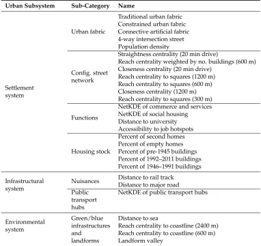
Table 2.The 28 features of the urban environment selected by the SFS technique, categorised by main urban subsystems, and sub-categories of subsystems.
Urban Subsystem Sub-Category Name
Settlement system
Urban fabric
Traditional urban fabric Constrained urban fabric Connective artificial fabric 4-way intersection street Population density
Config. street network
Straightness centrality (20 min drive)
Reach centrality weighted by no. buildings (600 m) Closeness centrality (20 min drive)
Reach centrality to squares (1200 m) Reach centrality to squares (600 m) Closeness centrality (1200 m) Reach centrality to squares (300 m)
Functions
NetKDE of commerce and services NetKDE of social housing
Distance to university Accessibility to job hotspots
Housing stock
Percent of second homes Percent of empty homes Percent of pre-1945 buildings Percent of 1992–2011 buildings Percent of 1946–1991 buildings
Infrastructural system
Nuisances Distance to rail track Distance to major road Public
transport hubs
NetKDE of public transport hubs
Environmental system Green/blue infrastructures and landforms
Distance to sea
Figure 3.Feature selection process.
3.4.2. GB Model
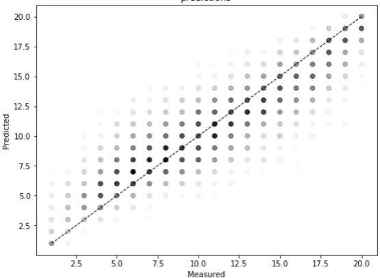
To model the relationship between the 28 features selected by the SFS technique and street value, we performed the following steps. Firstly, we split the data into training (80%) and test (20%) sets. Secondly, we set the hyperparameters of the GB regressor. More specifically, we set the maximum number of features to consider at each split and the maximum depth of each tree to a third of such number, a value commonly accepted in ML modelling [55]. Finally, we set to 128 the number of decision trees used by the algorithm. All these hyperparameters were double-checked through visual inspections of the learning curves. Finally, we set the mean squared error with improvement score by Friedman to measure the quality of each split in the decision trees and a 10-fold cross-validation. The resulting model had an average mean squared error of 1.05 for the training sets and 2.43 for the test sets. The adjustedR2values were 0.95 for the former and 0.75 for the latter, indicating that the 28 features chosen by the SFS technique could explain 75% of the variance of street value. In Figure4, we present the plot of the predicted versus real values. In Figure5, we present a map of the predicted street values in the study area under exam.
Figure 5.Predicted street-level valorisation of the housing market in the French Riviera.
As we explained above, spatial autocorrelation in the residuals of a GB model can help to identify missing explanatory features. To try to fully explain the spatial phenomenon under exam (i.e., the street values), we thus used the topological version of the Moran’s test presented in the Methodology as an exploratory tool to add further estimators to the ones selected by the SFS technique. If the Moran’s
I, in the residuals of a model obtained through a specific set of features, were to be significant at 10 topological steps (i.e., 10 street segments), we added an estimator that quantified a local phenomenon. Conversely, if the Moran’sIwere to be significant at a distance of 20 topological steps, we added an estimator that accounted for a more global phenomenon. This, together with an inspection of the map of the residuals, was helpful, for example, to identify the metric distance to university, a local aspect that was missing from the model and was important to explain the target feature. The output of the Moran’s test for the final model was as follows. At 10 topological steps, the Moran’sIwas 0.13 and statistically significant (i.e.,p-value = 0.0099), meaning that there were still traces of SA in the residuals and that some local explanatory variables were still missing. However, we could not access more data that would have allowed us to compute and test further metrics (e.g., data on housing stock at finer level of spatial granularity). At 20 topological steps, SA was significant but almost absent (i.e., Moran’sI= 0.08,p-value = 0.0099). We thus did not consider it necessary to calculate further metrics to quantify aspects at a larger scale.
3.4.3. Interpretations
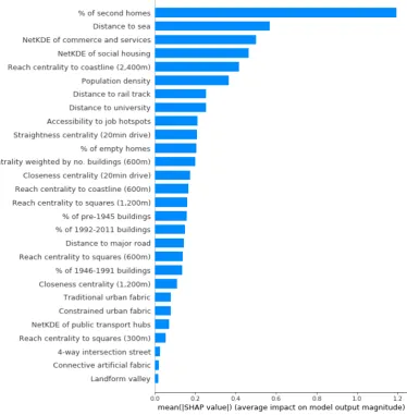
output magnitude (values in tabular format are provided in the AppendixA, in TableA1), and Figure7, which summarises, through a density scatter plot, the impacts (positive and negative) that each of the features used in the model had on street values. Vertical dispersion of points corresponds to a high concentration of observations with similar SHAP values. On the other hand, a slim dispersion corresponds to a small concentration of observations with similar SHAP values.
Figure 7.Summary plot of the impacts of the features used in the model.
computed on the street network at 800 m, had positive impacts on the valuation of streets for smaller values of such measure, while had negative effects for greater ones. The interpretation of this regressor is straightforward: greater concentrations of social housing contribute to the depreciation of the streets that surround them. We argue that this phenomenon is due to the social stigma usually assigned to such places. This finding is corroborated by previous works that found significant relationships between house prices discounts and proximity to social housing estates [56,57].
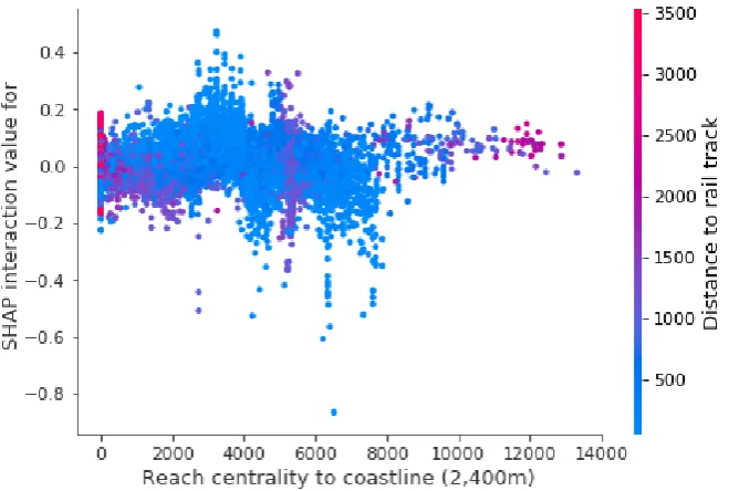
Impacts on street values for the remaining features were less polarised, meaning that great or small values of a specific estimator had both positive and negative effects on the valuations at the street level. Reach centrality at 2400 m with coastline as target tended to have positive effects on street values for greater centrality values (i.e., street that are at easy reach from the coast are more likely to have greater appreciations). Conversely, it tended to produce negative impacts on valuations at the street level for smaller values of reach. This finding was expected as the more a street is at easy reach from the coast, the higher its value should be. However, the distribution of negative and positive impacts with respect to the values of this measure was not neat as many observations with medium to high levels of reach centrality were actually associated with negative SHAP values. We hypothesise that the reason for this is related to the presence of rail tracks on many traits of the coastline of the French Riviera. To be more specific, the combination being close to the coastline, but not directly on it, and being close to a rail track depressed street values. The dependence plot (Figure8) between the measure of reach and the one of distance to rail track seems to confirm this hypothesis since negative SHAP interaction values are associated with higher levels of reach centrality than the average (but not in the top of the distribution) and short distances to rail tracks (i.e., between 0 and 500 m). This finding highlights the importance of using techniques that can handle non-linearity and interactions among features as they allow the investigation of complex relationships.
Figure 8.Dependence plot of reach centrality to coastline at 2400 m and distance to rail track.
respect to the others. For what regards accessibility to job hotspots (see the Supplementary Materials for details on how this metric was computed), SHAP values vary between−1 and 1, suggesting that higher levels of accessibility to job hotspots had positive effects on street values, while lower levels had negative ones. This finding is aligned with a previous study that found a relationship between residential valorisation and job accessibility (see, for example, the work by Osland and Thorsen [58]).
Finally, straightness centrality at 20 min drive, a measure of street network performance at 20 min drive radius, was associated with positive impacts on values at the street level for smaller values, while it was related to negative effects for greater values. This suggests that streets that are highly performing and thus function as pure connective elements (e.g., major routes near airports, important infrastructural nodes) tend to be devalued. We hypothesise that this might be due to the unpleasantness of the urban environment surrounding such streets, but also to air, noise pollution, and possible congestion.
Further estimators were used in the model; however, they had weaker impacts on street values. For example, reach centrality weighted by the number of buildings in each street segment and computed at 600 m radius showed that areas with a more sparse street network tended to be more valued than areas with a denser street layout. Reach centrality at 600 m with coastline as target specified at a more local scale the relationship found at 2400 m, highlighting the positive effects on values of the capes of the French Riviera (i.e., Cap d’Ail, Cap Ferrat, and Cap d’Antibes). Greater percentages of buildings built between 1946 and 1991 seemed to affect negatively street values, as compared to buildings built before the war or after 1992. For what concerns the metrics of urban fabric computed through the MFA method [33], only probability of MFA class 2 (i.e., streets with high probability of representing the traditional urban fabric) positively affected street values.
4. Limitations
Although PERVAL is an official dataset managed and kept updated by the French association of notaries, the geolocalisation of some observations might still be imprecise. Furthermore, Casanova et al. remarked that some housing transactions are missing in PERVAL and that particular attention should be given to the treatment of transactions concerning several items [59]. These issues might have thus introduced inaccuracies in the computation of our metric of street value.
By focusing on spatial units comprising of each street and immediate neighbouring streets with more than 10 transactions, we lost part of the information present in the original housing transaction dataset. Although we have done so to make our findings more statistically robust, such data might have helped to provide a more complete picture of the relationship between our metrics of the urban environment and values at the street level. In this respect, our findings are to be considered limited to the best known sub-spaces of the study area (in terms of recorded transactions).
Some limitations also come from the use of the ensemble ML method. The hyperparameters of the GB model were set through a trial and error process based on a visual evaluation of learning curves. Although this proved to be a valid technique in the specific case of the application presented in this paper, it is also time consuming and, to a certain extent, imprecise. For example, to better tune the maximum number of features that the GB model uses at each split, one could implement a cross validated grid search, an automatic algorithm that iteratively tests different numbers of features and outputs an optimal number for any given model, in a cross validated regime.
As pointed out in the Application Section, local SA is not completely absent from the residuals of the best model we could achieve. While this does not invalidate the results obtained, it informs us that potential explanatory variables are still missing.
5. Future Work
finer level of spatial granularity) to compute and test further local metrics that can reduce or completely eliminate SA at the local level and also increment the amount of explained variance in our model.
The methodology presented in this paper proposes analysing the relationship between features of the urban environment and a metric of street value based on the computation of ventiles of housing prices, which were previously harmonised to account for their heterogeneity. However, more street-based metrics can potentially be extracted from housing transaction data and tested against the metrics of the urban environment. For example, future work might consider a measure of dispersion of values, which could provide relevant information on whether specific streets are able to offer a range of housing values, and thus eventually be more prone to social mix.
Finally, uncertainty-based approaches such as Bayesian probabilities and possibility theory could be used to integrate the observations that were excluded in this analysis due to the requirements of the proposed methodology. Streets with few transactions could provide uncertain information on their median valorisation, but still contribute to gain a better understanding of how factors of the urban environment can contribute to the valorisation of streets in urban space.
6. Conclusions
Previous quantitative studies in the fields of urban design and urban morphology have investigated the relationship between aspects of the urban environment and socioeconomic as well as liveability aspects. However, such studies focused on single relationships (e.g., street network accessibility and socioeconomic levels) and thus did not consider the complex nature of the urban realm. A more recent quantitative methodology did propose a multivariate analysis of the relationship between multiple aspects of the urban environment and socioeconomic indexes. However, it was limited as: (i) it described the urban environment through a small number of descriptors; (ii) it proposed the use of areal units of analysis, rather than more fine grained ones, better associated with configurational and morphological aspects of cities; and (iii) it assumed linearity and independence among variables, while it might well be that urban phenomena do not behave in a linear manner and do have interactions.
In this paper, we propose a quantitative methodology to study the relationship between features of the urban environment and street value that overcomes previous limitations by: (i) providing detailed indications on the many aspects that could be included in the model (as the application showed, these can reach the hundreds); (ii) using the street segment as spatial unit of analysis; and (iii) implementing an ensemble of ML techniques (i.e., SFS, GB, topological Moran’s test, and SHAP) that handles non-linearity and interactions among variables, addresses issues of spatial autocorrelation in model residuals, and outputs interpretable results.
Such methodology was tested to analyse the relationship between 111 features of the urban environment and street values, obtained from the aggregation of around 110,000 housing transactions exchanged in the French Riviera, in the period 2008–2017. The model could explain up to 75% of the variance of the target variable and provided insightful information on the nuanced relationships existing among the selected features and street values. For example, reach centrality to the coast, which should theoretically hold a constant and positive relationship with street values, did not behave constantly across the study area due to an interaction effect with distance to rail track that ultimately depressed street values.
Supplementary Materials:The following are available online athttp://www.mdpi.com/2413-8851/3/3/100/s1.
Author Contributions: Conceptualisation, G.F., A.T. and A.V.; methodology, A.V.; software, A.V. and D.E.; validation, G.F. and D.E.; formal analysis, A.V. and D.E.; investigation, A.V. and D.E.; data curation, A.V. and D.E.; writing—original draft preparation, A.V.; writing—review and editing, G.F. and A.V.; visualisation, A.V.; supervision, G.F. and A.T.; project administration, G.F.; and funding acquisition, G.F.
Funding:This research was funded by the IDEX UCA JEDI, within the AAP Partenariat 2016 (action 6.5).
Acknowledgments: The authors of this paper would like to thank: data scientist Guillaume Ereteo for indispensable inputs on ML techniques and for having implemented and tested the first version of the algorithm presented in this paper; Denis Overal, director of the R&D at Kinaxia, for his supervision and insightful inputs that permitted the smooth advancement of the research project; PhD candidate Alessandro Araldi, who helped with the computation of some of the metrics used in this work; and, finally, Diego Moreno and Karine Emsellem, professors of Geography at the University of Nice, for their insightful observations, in the brainstorming phase of the research project.
Conflicts of Interest:The authors declare no conflict of interest.
Abbreviations
The following abbreviations are used in this manuscript:
ML Machine Learning GB Gradient Boosting
SHAP SHapley Additive exPlanations MFA Multiple Fabric Assessment NetKDE Network Kernel Density Estimation SFS Sequential Forward Selection RF Random Forests
SA Spatial Autocorrelation OSM OpenStreetMap DEM Digital Elevation Model
IGN Institut National de l’Information Géographique et Forestière (National Institute of Geography and Forestry) INSEE Institut National de la Statistique et des Etudes Economiques (National Institute of Statistics and Economic Studies) PM Petites Maisons (Small Houses)
GM Grandes Maisons (Big Houses)
Appendix A
Appendix A.1
The 111 metrics of the urban environment used in the analysis presented in this paper, including categorisation in subsystems, names, brief descriptions, and observed values are provided in the Supplementary Materials.
Appendix A.2
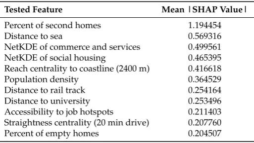
Table A1. Average impacts (i.e., SHAP values) in absolute terms of the features on the model output magnitude.
Tested Feature Mean |SHAP Value|
Percent of second homes 1.194454
Distance to sea 0.569316
NetKDE of commerce and services 0.499561 NetKDE of social housing 0.465395 Reach centrality to coastline (2400 m) 0.416618
Population density 0.364529
Distance to rail track 0.254164
Distance to university 0.253496
Accessibility to job hotspots 0.211403 Straightness centrality (20 min drive) 0.207760
Table A1.Cont.
Tested Feature Mean |SHAP Value|
Reach centrality weighted by No. buildings (600 m) 0.198957 Closeness centrality (20 min drive) 0.174979 Reach centrality to coastline (600 m) 0.166626 Reach centrality to squares (1200 m) 0.161731
Percent of pre-1945 buildings 0.157978
Percent of 1992–2011 buildings 0.149031
Distance to major road 0.144553
Reach centrality to squares (600 m) 0.139323
Percent of 1946–1991 buildings 0.134130
Closeness centrality (1200 m) 0.108757
Traditional urban fabric 0.080152
Constrained urban fabric 0.080079
NetKDE of public transport hubs 0.069642
Reach centrality to squares (300 m) 0.053538
4-way intersection street 0.024855
Connective artificial fabric 0.019045
Landform valley 0.017471
References
1. Vaughan, L.; Clark, D.L.C.; Sahbaz, O.; Haklay, M. Space and exclusion: Does urban morphology play a part in social deprivation?Area2005,37, 402–412. [CrossRef]
2. Hillier, B. Can streets be made safe? Urban Des. Int.2004,9, 31–45. [CrossRef]
3. Harries, K. Property Crimes and Violence in United States: An Analysis of the influence of Population density. Int. J. Crim. Justice Sci.2006,1, 24–34.
4. Hillier, B.; Sahbaz, O. An Evidence Based Approach to Crime and Urban Design. Or, Can We Have Vitality, Sustainability and Security All at Once; Bartlett School of Graduates Studies University College London: London, UK, 2008.
5. Duany, A.; Plater-Zyberk, E.; Speck, J.Suburban Nation: The Rise of Sprawl and the Decline of the American Dream; Macmillan: New York, NY, USA, 2001.
6. Burchell, R.W.; Shad, N.A.; Listokin, D.; Phillips, H.; Downs, A.; Seskin, S.; Davis, J.S.; Moore, T.; Helton, D.; Gall, M. The Costs of Sprawl-Revisited. Number Project H-10 FY’95. 1998. Available online: http:// onlinepubs.trb.org/onlinepubs/tcrp/tcrp_rpt_39-a.pdf(accessed on 12 September 2019).
7. Conzen, M.R.G. Alnwick, Northumberland: A study in town-plan analysis. Trans. Pap. (Inst. Br. Geogr.) 1960,27, iii–122. [CrossRef]
8. Caniggia, G.; Maffei, G.L.Architectural Composition and Building Typology: Interpreting Basic Building; Alinea Editrice: Firenze, Italy, 2001; Volume 176.
9. Venerandi, A.; Quattrone, G.; Capra, L. A scalable method to quantify the relationship between urban form and socio-economic indexes. EPJ Data Sci.2018,7, 4. [CrossRef]
10. Carmona, M. Place value: Place quality and its impact on health, social, economic and environmental outcomes.J. Urban Des.2019,24, 1–48. [CrossRef]
11. Hillier, B.Space Is the Machine: A Configurational Theory of Architecture; Space Syntax: London, UK, 2007. 12. Shearmur, R.; Charron, M. From Chicago to LA and back again: A Chicago-inspired quantitative analysis
of income distribution in Montreal.Prof. Geogr.2004,56, 109–126.
13. Rosen, S. Hedonic prices and implicit markets: Product differentiation in pure competition.J. Political Econ. 1974,82, 34–55. [CrossRef]
14. Orford, S. Modelling spatial structures in local housing market dynamics: A multilevel perspective. Urban Stud.2000,37, 1643–1671. [CrossRef]
15. Law, S. Defining Street-based Local Area and measuring its effect on house price using a hedonic price approach: The case study of Metropolitan London.Cities2017,60, 166–179. [CrossRef]
17. Caplin, A.; Chopra, S.; Leahy, J.V.; LeCun, Y.; Thampy, T. Machine Learning and the Spatial Structure of House Prices and Housing Returns. Available at SSRN 1316046 2008. Available online:http://yann.lecun. com/exdb/publis/pdf/caplin-ssrn-08.pdf(accessed on 12 September 2019).
18. Sommervoll, Å.; Sommervoll, D.E. Learning from man or machine: Spatial fixed effects in urban econometrics. Reg. Sci. Urban Econ.2019,77, 239–252. [CrossRef]
19. Porta, S.; Crucitti, P.; Latora, V. The network analysis of urban streets: A primal approach.Environ. Plan. B Plan. Des.2006,33, 705–725. [CrossRef]
20. Batty, M. Cities as Complex Systems: Scaling, Interaction, Networks, Dynamics and Urban Morphologies; Springer: Berlin, Germany, 2009.
21. Hofman, J.M.; Sharma, A.; Watts, D.J. Prediction and explanation in social systems. Science2017, 355, 486–488. [CrossRef] [PubMed]
22. Carpenter, A.; Peponis, J. Poverty and connectivity. J. Space Syntax2010,1, 108–120.
23. Gourdon, J.L. La rue: Essai sur l’économie de la forme urbaine; Editions de l’Aube: La Tour-d’Aigues, France, 2001.
24. Hillier, B. Cities as movement economies. Urban Des. Int.1996,1, 41–60. [CrossRef]
25. Bourdieu, P.La distinction. Critique Sociale du Jugement; Les Editions de Minuit: Paris, France, 1979. 26. Ærø, T. Residential choice from a lifestyle perspective. Hous. Theory Soc.2006,23, 109–130. [CrossRef] 27. Kauko, T. Expressions of housing consumer preferences: Proposition for a research agenda.
Hous. Theory Soc.2006,23, 92–108. [CrossRef]
28. Luttik, J. The value of trees, water and open space as reflected by house prices in the Netherlands. Landsc. Urban Plan.2000,48, 161–167. [CrossRef]
29. Bartholomew, K.; Ewing, R. Hedonic price effects of pedestrian-and transit-oriented development. J. Plan. Lit.2011,26, 18–34. [CrossRef]
30. Brainard, J.S.; Jones, A.P.; Bateman, I.J.; Lovett, A.A.; Fallon, P.J. Modelling environmental equity: Access to air quality in Birmingham, England. Environ. Plan. A2002,34, 695–716. [CrossRef]
31. Berghauser-Pont, M.; Haupt, P. SPACEMATRIX, Space, Density and Urban Form; NAi Publishers: Amsterdam, The Netherlands, 2010.
32. Gil, J.; Beirão, J.N.; Montenegro, N.; Duarte, J.P. On the discovery of urban typologies: Data mining the many dimensions of urban form.Urban Morphol.2012,16, 27.
33. Araldi, A.; Fusco, G. From the street to the metropolitan region: Pedestrian perspective in urban fabric analysis. Environ. Plan. B Urban Anal. City Sci.2019,46, 1243–1263. [CrossRef]
34. Venerandi, A.; Zanella, M.; Romice, O.; Dibble, J.; Porta, S. Form and urban change–An urban morphometric study of five gentrified neighbourhoods in London. Environ. Plan. B Urban Anal. City Sci. 2017,44, 1056–1076. [CrossRef]
35. Porta, S.; Crucitti, P.; Latora, V. Multiple centrality assessment in Parma: A network analysis of paths and open spaces. Urban Des. Int.2008,13, 41–50. [CrossRef]
36. Wang, F.; Antipova, A.; Porta, S. Street centrality and land use intensity in Baton Rouge, Louisiana. J. Transp. Geogr.2011,19, 285–293. [CrossRef]
37. Porta, S.; Latora, V.; Wang, F.; Rueda, S.; Strano, E.; Scellato, S.; Cardillo, A.; Belli, E.; Cardenas, F.; Cormenzana, B.; et al. Street centrality and the location of economic activities in Barcelona.Urban Stud. 2012,49, 1471–1488. [CrossRef]
38. Okabe, A.; Sugihara, K.Spatial Analysis along Networks: Statistical and Computational Methods; John Wiley & Sons: Hoboken, NJ, USA, 2012.
39. Fusco, G.; Caglioni, M.; Araldi, A. Street network morphology and retail locations. Application to the city of Nice (France). Plurimondi2015,17, 15–22.
40. Tagil, S.; Jenness, J. GIS-based automated landform classification and topographic, landcover and geologic attributes of landforms around the Yazoren Polje, Turkey. J. Appl. Sci.2008,8, 910–921. [CrossRef] 41. Raschka, S. MLxtend: Providing machine learning and data science utilities and extensions to Python’s
scientific computing stack.J. Open Source Softw.2018,3. [CrossRef]
42. Friedman, J.H. Greedy function approximation: A gradient boosting machine. Ann. Stat. 2001, 29, 1189–1232. [CrossRef]
44. Legendre, P. Spatial autocorrelation: Trouble or new paradigm? Ecology1993,74, 1659–1673. [CrossRef] 45. Moran, P.A. Notes on continuous stochastic phenomena. Biometrika1950,37, 17–23. [CrossRef] [PubMed] 46. Lundberg, S.M.; Lee, S.I. A unified approach to interpreting model predictions. In Advances in Neural
Information Processing Systems; The MIT Press: Cambridge, MA, USA, 2017; pp. 4765–4774.
47. Lundberg, S.M.; Erion, G.G.; Lee, S.I. Consistent individualized feature attribution for tree ensembles. arXiv2018, arXiv:1802.03888.
48. Perval. Available online:https://www.perval.fr(accessed on 31 July 2019).
49. BD TOPO. Available online:http://professionnels.ign.fr/bdtopo(accessed on 31 July 2019).
50. Base Sirene des entreprises et de leurs établissements. Available online:https://www.data.gouv.fr/fr/ datasets/base-sirene-des-entreprises-et-de-leurs-etablissements-siren-siret/(accessed on 31 July 2019). 51. Logement en 2014. Available online: https://www.insee.fr/fr/statistiques/3137421 (accessed on 31
July 2019).
52. OpenMobilityData. Available online: https://transitfeeds.com/l/541-nice-france (accessed on 31 July 2019).
53. OpenStreetMap (OSM). Available online:https://www.openstreetmap.org/(accessed on 31 July 2019). 54. GEOFABRIK Downloads. Available online:http://download.geofabrik.de(accessed on 31 July 2019). 55. Trevor, H.; Robert, T.; JH, F. The Elements of Statistical Learning: Data Mining, Inference, and Prediction;
Springer: Berlin, Germany, 2009.
56. Grether, D.M.; Mieszkowski, P. The effects of nonresidential land uses on the prices of adjacent housing: Some estimates of proximity effects.J. Urban Econ.1980,8, 1–15. [CrossRef]
57. Du Preez, M.; Sale, M. The Impact of Social Housing Developments on Nearby Property Prices: A N elson M andela B ay Case Study. S. Afr. J. Econ.2013,81, 451–466. [CrossRef]
58. Osland, L.; Thorsen, I. Effects on housing prices of urban attraction and labor-market accessibility. Environ. Plan. A2008,40, 2490–2509. [CrossRef]
59. Casanova, L.; Boulay, G.; Gérard, Y.; Yahi, L. Deux bases de données, aucune référence de prix. Revue d’Economie Regionale Urbaine2017,4, 711–732. [CrossRef]
c