www.nonlin-processes-geophys.net/18/243/2011/ doi:10.5194/npg-18-243-2011
© Author(s) 2011. CC Attribution 3.0 License.
Nonlinear Processes
in Geophysics
On the Kalman Filter error covariance collapse
into the unstable subspace
A. Trevisan1and L. Palatella2
1Istituto di Scienze dell’Atmosfera e del Clima del CNR, via Gobetti 101, 40129 Bologna, Italy
2Istituto di Scienze dell’Atmosfera e del Clima del CNR, UdR di Lecce, via Lecce-Monteroni, km 1,200, 73100 Lecce, Italy Received: 9 February 2011 – Revised: 10 March 2011 – Accepted: 21 March 2011 – Published: 28 March 2011
Abstract. When the Extended Kalman Filter is applied to
a chaotic system, the rank of the error covariance matri-ces, after a sufficiently large number of iterations, reduces toN++N0whereN+ andN0are the number of positive and null Lyapunov exponents. This is due to the collapse into the unstable and neutral tangent subspace of the solution of the full Extended Kalman Filter. Therefore the solution is the same as the solution obtained by confining the assimila-tion to the space spanned by the Lyapunov vectors with non-negative Lyapunov exponents. Theoretical arguments and numerical verification are provided to show that the asymp-totic state and covariance estimates of the full EKF and of its reduced form, with assimilation in the unstable and neu-tral subspace (EKF-AUS) are the same. The consequences of these findings on applications of Kalman type Filters to chaotic models are discussed.
1 Introduction
This work is motivated by the problem of data assimilation in meteorology and oceanography. Atmospheric and oceanic observations are noisy and very scattered in space and time. Dynamical models describing the evolution of the state of the atmosphere and the ocean are chaotic and, moreover, the number of degrees of freedom is huge (>108). In the Earth sciences, the classical problem of estimating the state from noisy and incomplete observations and the approximate knowledge of the equations governing the system’s evolution is known as data assimilation.
Data assimilation methods can be classified in two cat-egories: sequential and variational, the most notable in the two classes being Kalman Filters and four-dimensional
Correspondence to: A. Trevisan
(a.trevisan@isac.cnr.it)
variational assimilation (4DVar), respectively (Ghil and Malanotte-Rizzoli (1991); Kalnay (2003) and references therein). 4DVar is an advanced technique that seeks the model trajectory that best fits the observations distributed within a given time interval with the dynamical constraint of the model equations (Talagrand and Courtier, 1987). The op-timal control theory (Le Dimet and Talagrand, 1986) allows the minimization of the 4D-Var cost function to be made with respect to the state at the beginning of the interval. The solu-tion of the minimizasolu-tion problem is obtained by forward inte-gration of the model and backward inteinte-gration of the adjoint of the tangent linear propagator that yields the expression of the cost function gradient.
The Kalman Filter was originally developed for linear sys-tems. Based on information about the error covariance of the data and model forecast, the KF provides the optimal linear estimate of the state of the system. A straightforward way of extending the linear results to the nonlinear case is given by the Extended Kalman Filter (EKF) (Jazwinski, 1970; Miller et al., 1994): in the EKF the error covariance is propagated in time according to linearized model dynamics. In the fore-cast step the nonlinear model is integrated, starting from the previous analysis to obtain the background state, and the tan-gent linear equations propagate the analysis error covariance to obtain an estimate of the background error covariance. When observations become available they are assimilated in the analysis step that combines the background and the ob-servations with the appropriate weights. The error covariance associated with the state estimate at the analysis step is also updated.
Singular Value Decomposition (SVD), Eigenvalue Decom-position (EVD) or projection on the leading Empirical Or-thogonal Functions (Pham et al., 1998). A Monte Carlo approach, referred to as Ensemble Kalman Filter (EnKF) (Evensen, 1994), provides ensemble representations for the probability distribution of the state estimate. The EnKF has also proven effective in reducing the computational cost associated with the full EKF. In the EnKF, the ensemble-predicted error statistics are estimated from the ensemble perturbations. In the forecast step their evolution is computed as difference between nonlinear integrations of the model, a procedure similar to the breeding method (Toth and Kalnay, 1993, 1997). For sufficiently small analysis errors, this pro-cedure would give the same result as using the tangent linear propagator.
The various flavors of the Ensemble Kalman Filter (EnKF) testify the importance of this problem for real world ap-plications (see Blum et al., 2008; Kalnay, 2003 and refer-ences therein). These include several ad-hoc refinements as perturbing observations, covariance localization, additive or multiplicative inflation. In particular, covariance localization is beneficial to prevent filter divergence when the number of ensemble members is small (for a review see Evensen, 2003). In all these studies, how many members of the ensemble are needed is empirically estimated on a case to case basis.
Ott et al. (2004) estimate the local dimensionality (E-dimension) from the perturbations of the Local Ensemble Kalman Filter and the number of members of the ensem-ble necessary to represent the forecast error covariance in different geographical regions (tropics, extra-tropics, polar regions).
We consider the application of the EKF to a chaotic sys-tem and we concentrate on issues related to the dimension of its unstable subspace. So et al. (1994) addressed a similar problem in control theory; in reconstructing the state vec-tor of a chaotic system from the time series of an observed scalar, they showed that the control vector lies in the unsta-ble space. The Assimilation in the Unstaunsta-ble Subspace (AUS), developed by Trevisan and co-authors, consists in confining the analysis update to the subspace spanned by the leading unstable directions (Trevisan and Uboldi, 2004). Applica-tions to atmospheric and oceanic models (Uboldi and Tre-visan, 2006; Carrassi et al., 2008b) showed that even dealing with high-dimensional systems, an efficient error control can be obtained by monitoring only a limited number of unstable directions. The forecast error in these directions was esti-mated with empirical techniques. More recently, Trevisan et al. (2010) formulated a reduced subspace 4-dimensional as-similation algorithm, 4DVar-AUS (Four-dimensional Varia-tional Assimilation in the Unstable Subspace). The key result of this study is the existence of an optimal subspace dimen-sion for the assimilation that is approximately equal to the unstable and neutral subspace dimension.
The methodology of the present paper goes back to the roots of the filtering theory, the EKF, to address questions re-garding the number of degrees of freedom that describe the filter error evolution in a chaotic system of given unstable manifold dimension. In this work we first show how it is possible to define a mathematically rigorous algorithm with the following properties: the solution of the Kalman filter equations is reproduced when all degrees of freedom are con-sidered; with assimilation increments limited to a subspace of the tangent space, a reduced order algorithm is obtained where the estimated errors are confined to the most unstable subspace of the system. We will discuss the equivalence of the full EKF with its reduced form (EKF-AUS) with assim-ilation in the unstable and neutral space, i.e. the span of the firstN++N0Lyapunov vectors, whereN+andN0are the number of positive and null Lyapunov exponents. Then we compare numerical solutions obtained with the full EKF and the reduced algorithm EKF-AUS. Throughout the paper, the unified notation of (Ide et al., 1997) is used.
The results of this paper are based on the hypothesis that observations are accurate enough to ensure small analysis er-rors so that the erer-rors evolution is correctly described by the tangent linear operator. In practice these are the same pothesis of validity of the standard EKF algorithm. This hy-pothesis is crucial for all the considerations we will make regarding the Lyapunov exponents and vectors, since they are well-defined along the true trajectory while here we ex-tend their properties to the pseudo-trajectory determined by the forecast-analysis cycle. This is reasonable if the pseudo-trajectory remains close enough to the true pseudo-trajectory.
If the observations are so few and noisy that the analysis errors are large, the theoretical results of this paper do not apply directly. However, a straightforward generalization of the EKF-AUS algorithm to account for the nonlinear error behavior is possible, as discussed in the conclusions. Due to nonlinear error dynamics, the perturbations will not remain exactly in the unstable and neutral subspace and it may be necessary to use a larger subspace. Indeed the results ob-tained with the 4DVar-AUS algorithm (Trevisan et al., 2010) showed that, when observation errors are large enough that nonlinearity becomes important, the dimension of the sub-space where errors live also increases; in such case a larger number of perturbations is needed.
2 The extended Kalman Filter and its reduction to the unstable space
2.1 The extended Kalman Filter
noisyp-dimensional observations y0k=H(xk)+εkogiven at discrete timestk> t0,k∈ {1,2,...}. The observation errorεko is assumed to be Gaussian with zero mean and knownp×p covariance matrix R.His the observation operator. The es-timate update is given by the analysis equation:
xak=xfk −KkH(xfk)+Kkyok, (1) where xfk is the forecast obtained by integrating the model equations from a previous analysis time:
xfk =M(xak−1), (2)
Mbeing the nonlinear evolution operator. Kk is the gain
matrix at timetk given by: Kk=PfkHT
HPfkHT+R−1, (3)
where H is the Jacobian ofH. The analysis error covariance update equation is given by:
Pak=(I−KkH)Pfk, (4)
and Pfk, the forecast error covariance, is given by:
Pfk =MkPak−1MTk, (5)
where M is the linearized evolution operator associated with
M. We have assumed that there is no model error.
2.2 The algorithm EKF-AUS
We introduce an algorithm that belongs to the family of square-root implementations of the EKF (Thornton and Bier-man, 1976; Tippett et al., 2003). A reduced version is then obtained from the full rank algorithm. We perform the assim-ilation in a manifold of dimensionm. Whenmis equal to the numbernof degrees of freedom of the system, the algorithm solves the standard EKF equations.
We consider a chaotic system with a numberN+of pos-itive Lyapunov exponents andN0 of null Lyapunov expo-nents. Whenm=N++N0the reduced form, with Assimi-lation in the Unstable Subspace (EKF-AUS) is obtained.
At timet=tk−1, let then×mmatrix Xa be one of the square roots of Pa, namely Pa=XaXaT and let the columns of Xa= [δxa1,δxa2,...,δxam] be orthogonal. At time t=t0, the vectorsδxai,i=1,2,...,mare arbitrary independent ini-tial perturbations. (Here and in the following we drop the time-step subscript from the equations since, unless other-wise stated, all terms refer to the same time stepk).
In the standard EKF algorithm, the number of perturba-tions is equal to the total number of degrees of freedom of the system,m=n. In the reduced order algorithm referred to as EKF-AUS the number of perturbations is equal to the di-mension of the unstable and neutral manifold:m=N++N0
2.2.1 The forecast step
In the forecast step, the tangent linear operator M acts on the perturbations Xa defined at (analysis) time t=tk−1 (other terms in this and the following equations refer to time step t=tk):
Xf=MXa (6)
where Xf= [δxf1,δx2f,...,δxfm]. Then×nforecast error co-variance matrix:
Pf=XfXf T (7)
can be cast in the form:
Pf=Ef0fEf T (8)
where themcolumns of Ef are obtained by a Gram-Schmidt orthonormalization of the columns of Xf. The m×m (in general non-diagonal) symmetric matrix0f defined as:
0f=Ef TXfXf TEf (9)
represents the forecast error covariance matrix, confined to the subspaceSmof the evolved perturbations. In the standard EKF algorithm (m=n), Ef isn×nand its columns span the full space. In the reduced form algorithm, Ef isn×mand its columns span anm-dimensional subspaceSmof the entire phase space.
2.2.2 The analysis step
Using the definition of Pf of Eq. (8) the Kalman gain expres-sion becomes:
K=Ef0f(HEf)Th(HEf)0f(HEf)T+Ri
−1
(10) and the usual analysis error covariance update, Eq. (4) reads:
Pa=(I−KH)Ef0fEf T=Ef0fEf T+
−Ef0f(HEf)T
(HEf)0f(HEf)T+R−1
HEf0fEf T
=Efn0f−0fEf THT
(HEf)0f(HEf)T+R−1
×HEf0f Ef T≡Ef0a0Ef T
(11)
The analysis error covariance matrix Pacan be written as:
Pa=Ef0a0Ef T =EfU0aUTEf T
≡Ea0aEaT, (12)
where the columns of the(m×m)orthogonal invertible ma-trix U are the eigenvectors of the symmetric mama-trix0a0= U0aUT (to numerically obtain the eigenvalues and the eigen-vectors of0a0 we use the power iterations method (Golub et al., 1996)) and0a=diag[γi2]is diagonal. Therefore, them columns of Ea= [ea
1,e a
2,...,eam]obtained by
span the same subspace Sm as the columns of Ef. Con-sequently, the analysis step preserves the subspace Sm, an important point in the subsequent discussion (see Sec. 2.3) on the comparison of our scheme with the Benettin et al. (1980) algorithm. The square root of Pa, written as Pa= Ea0aEaT ≡XaXaT, provides a set of orthogonal vectors:
Xa=Ea(0a)1/2. (14)
The columns of
Xa= [γ1ea1,γ2e2a,...,γmeam] = [δxa1,δx a 2,....,δx
a
m] (15)
are the new set of perturbation vectors defined after the anal-ysis step at timetkthat enter the forecast step (6) at the next time steptk+1. Their amplitude is consistent with the analy-sis error covariance in the subspaceSm
Notice that, as in other Kalman square root filters, with the introduction of Eaand Ef, forming the full forecast and analysis error covariance matrices can be avoided. The anal-ysis equation is the usual Eq. (1) with K given by (10). When m=n, K is the usual Kalman gain. In EKF-AUS (m=N++N0) the analysis increment is confined to the sub-spaceSm spanned by the mcolumns of Ef in view of the form of K.
2.2.3 Numerical Implementation
In the numerical implementation of the algorithm one can start with a number of perturbationsmthat is at least as large asN++N0. If an independent estimate ofN++N0is not available one can start with an initial guess formthat is an overestimate ofN++N0. We now summarize the different steps of the EKF-AUS algorithm as they are performed in the numerical implementation:
1. we evolve the state vector xak−1with the full nonlinear model equations and then×mmatrix Xak−1 using the tangent linear operator Mk, as in Eq. (6), obtaining Xfk at time stepk
2. we orthonormalize themcolumns of Xfk obtaining the columns of Ef
3. we calculate them×mcovariance matrix0f through Eq. (9)
4. we perform the analysis on the state vector as in Eq. (1) with K given by Eq. (10)
5. we calculate m×m covariance matrix 0a0 that after Eq. (11) can be written as
0a0 =0f−0fEf THT
×
(HEf)0f(HEf)T+R−1
HEf0f. (16) (notice that the matrix to be inverted has the dimension pof the number of observations)
6. we diagonalize them×mmatrix0a0. We put the nor-malized eigenvectors of 0a0 in the orthogonalm×m matrix U and then we obtain Ea=EfU. Both Ef and Eaaren×m.
7. we multiply thei-th column of Eaby the square rootγi ofi-th eigenvalue of0aobtaining the new set of pertur-bations Xak.
2.3 Further discussion on the EKF-AUS algorithm
In summary, the EKF-AUS algorithm is obtained by reduc-ing the dimension of the subspace,Sm, where the analysis update, xa−xf and the estimated analysis and forecast er-ror covariance Paand Pf are confined. It will soon become clear whymis set equal to the dimension of the unstable and neutral subspace.
During the forecast step the error evolution is governed by Eq. (6). Suppose that at a certain time,tkthe firstN++N0of themperturbations are confined to the unstable and neutral subspace, that is the columns of Easpan the same subspace as the leadingN++N0Lyapunov vectors. After the fore-cast step, this subspace is mapped into the unstable subspace referred to the state xf at timetk
+1. The new perturbations
Xf are amplified but they are still confined in the subspace of the leadingN++N0Lyapunov vectors. These perturbations will survive throughout the long time assimilation process. The remainingm−N+−N0perturbations, being recurrently orthogonalized, are deprived of the component along the un-stable manifold like in the Benettin et al. (1980) algorithm, while the component along the stable manifold is damped during the forecast (the validity of this reasoning does not re-quire the orthogonality of the stable and unstable manifolds). The main difference between our algorithm and that of Benettin et al. (1980) is introduced in the analysis step. In our algorithm, use is made of Eq. (11) to redefine the pertur-bations. These are confined by construction to the subspace spanned by the columns Ef and after the analysis step the span of the columns of Ea and of the columns of Xa will be the same space spanned by the columns of Ef as shown in Sect. 2.2.2. For a detailed proof of this fact we refer to Appendix A.
Another difference from (Benettin et al., 1980) is that in our case the vectors at the end of the analysis step are or-thogonal but not orthonormal, so that perturbations that are damped during the forecast are not artificially “kept alive” (as it happens with the orthonormalization step of Benettin et al., 1980). The(I−KH)term has a stabilizing effect that tends to reduce the amplitude of perturbations in view of the existence of observations (Carrassi et al., 2008). As a conse-quence, when the amplitude of perturbations is redefined af-ter the analysis step the decaying modes are further damped while the unstable modes are kept from diverging.
analysis steps will, in the long run, be confined to the unsta-ble and neutral subspace. In view of this reasoning, based on the linearization of the error dynamics, it is argued that the EKF and EKF-AUS algorithms will asymptotically produce the same estimate of error covariances. The numerical results confirm the validity of these statements.
¿From previous considerations, if we choose an initial number of perturbationsm > N++N0,m−N+−N0 pertur-bations will be damped by the assimilation process. On the contrary, if we choosem < N++N0, some unstable direc-tions will be ignored and, consequently, the filter will even-tually diverge.
3 Numerical results
We now compare the numerical results obtained with the re-duced EKF-AUS algorithm with those obtained with the full EKF, when the EKF algorithm itself is stable and no filter divergence is observed. Experiments are based on Lorenz96 model (Lorenz, 1996), that has been widely used for testing data assimilation algorithms. The governing equations are:
d
dtxj=(xj+1−xj−2)xj−1−xj+F (17) withj=1,...,n. The variables xj represent the values of a scalar meteorological quantity at n equally spaced geo-graphic sites on a periodic longitudinal domain. The model has chaotic behavior for the value of the forcing,F=8, used in most studies. The number of variablesnof the model is varied to obtain different systems with a different number of degrees of freedom and, consequently, a different number of positive Lyapunov exponents. Withn=40,60,80 the sys-tems have 13,19,25 positive Lyapunov exponents, respec-tively.
All simulations are performed in a perfect model scenario, that is a trajectory on the attractor of the system is assumed to represent the true state evolution. Observations are cre-ated by adding uncorrelcre-ated random noise with Gaussian dis-tribution (zero mean, variance σ02) to the true state. The assimilation experiments with EKF and EKF-AUS use the same reference trajectory and the same observations. The performance of the assimilation is measured by the analy-sis error, the root mean square (rms) of the difference be-tween the true and the estimated state vectors. Observations are taken at discrete times corresponding to the assimilation timestk. Results shown refer to the following parameters but different choices of observational configurations gave quali-tatively similar results. The time interval between observa-tions is 0.05 (=4 time integration steps); every other grid point is observed and the observation points are shifted by one at each observation time.
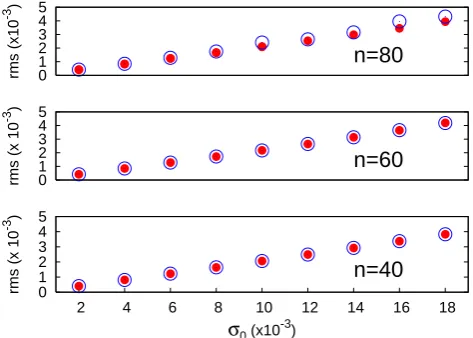
Figure 1 shows the rms estimation error for the three sys-tems (n=40,60,80) as a function of the observation error standard deviation,σ0. Values are in the range 0.002≤σ0≤
0 1 2 3 4 5
2 4 6 8 10 12 14 16 18
rms (x 10
-3 )
σ0 (x10 -3
)
n=40
0 1 2 3 4 5
rms (x 10
-3 )
n=60
0 1 2 3 4 5
rms (x10
-3 )
n=80
Fig. 1. Average root mean square error of the algorithms: EKF (full
circles), EKF-AUS (empty circles) for systems withn=40,60,80
degrees of freedom, as a function ofσ0, the observation error
stan-dard deviation. The average was performed over 1000 assimilation steps (50 time units) after a stabilization period of the same length.
0.018 where filter divergence is not observed; for values of σ0>0.02, divergence possibly occurs in both EKF and EKF-AUS algorithms. The rms error was averaged over 1000 suc-cessive assimilation times or 50 time units, after waiting a transient time of 50 time units for the filter error to stabilize. The sets of points displayed in the figure refer to EKF and EKF-AUS, (m=14,20,26) and show that the average error is statistically the same. The results show that, in agreement with the theory, for sufficiently small values ofσ0, error dy-namics is linear and the estimation error grows linearly with the observation error. Notice also that the asymptotic aver-age error is about the same in the three model configurations withn=40,60,80. This is because the number of unstable directions is proportional to the extension of the spatial do-main and the number of observations that can detect them increases by the same proportion.
10 15 20 25 30 35 40
0 10 20 30 40 50 60 70 80 90 100
P
a rank
Time
n=40 n=60 n=80
Fig. 2. Rank of the analysis error covariance matrix Pain the EKF
algorithm. Forn=40,60,80, the dimension of the unstable and
neutral space is 14,20,26, respectively.σ0=0.01.
The analysis error covariance matrix was explicitly written in Eq. (12) in terms of the orthonormal basis Eaof the anal-ysis error, the eigenvalues of0a being the error variances in this subspace; this formulation was useful to interpret the behavior of the error covariance in the stable and unstable directions. The estimated errors in the stable directions are damped during the forecast step and are reduced by the ef-fect of the(I−KH)term at analysis step. We conclude that only errors in the unstable directions, that amplify during the forecast step, can survive along the sequence of successive forecast and analysis iterations.
The numerical results confirm this argument: the rank of the error covariance matrix of the EKF decreases until it reaches a value consistent with the expectation that, in the long run, only the unstable or weekly stable error compo-nents remain active. At the same time, the reduction of the rank of Pain the EKF explains the long-term equivalence in the performance of EKF and EKF-AUS: the subspace dimen-sion of the covariance matrices in the two algorithms become asymptotically the same. Further numerical evidence of va-lidity of the theory is provided by the spectrum of eigenval-ues of the error covariance matrices. Fig. 3, obtained in the same numerical settings of Figs. 1 and 2, shows the eigenval-ues of Pafor EKF and of0afor EKF-AUS computed at the final time of Fig. 2. The eigenvalues obtained with the two algorithms, in logarithmic scale in the figure, are the same within numerical accuracy.
The above results explain why the two algorithms, EKF and EKF-AUS, after a transient stage start to behave in a similar fashion and asymptotically give the same numerical analysis solution.
1e-11 1e-10 1e-09 1e-08 1e-07 1e-06 1e-05 0.0001
0 5 10 15 20 25 30
P
a Eigenvalue
Eigenvalue no. AUS n=40
EKF n=40 AUS n=60 EKF n=60 AUS n=80 EKF n=80
Fig. 3. Eigenvalues of the analysis error covariance matrix at final time of assimilation with: EKF (full) and EKF-AUS (empty) for
systems withn=40,60,80.σ0=0.01.
4 Conclusions
We considered a system with a chaotic attractor and studied the consequences of the existence of an unstable manifold on the evolution of filter solution error. The algorithm we pre-sented reproduces exactly the EKF equations when all de-grees of freedom are considered. The idea of confining the assimilation in the invariant unstable and neutral subspace is not new and was exploited in a series of papers, including the formulation of the 4DVar-AUS algorithm (Trevisan et al., 2010); it was the original purpose of the present work to ap-ply the same idea to the Kalman Filter. The most important and new result of the paper, not foreseen by the authors them-selves, is that the exended Kalman Filter solution collapses into this invariant subspace so that its solution is not different from the solution of the reduced form of the algorithm (EKF-AUS). More specifically, the EKF algorithm and EKF-AUS algorithm with a number of degrees of freedom equal to the number of positive and neutral exponents produce the same asymptotic state and error covariance estimates. In a sense the EKF solution converges to the EKF-AUS solution, not viceversa. This happens because the rank of the full EKF error covariance matrices asymptotically becomes as small as the dimension of the unstable and neutral manifold of the original system equations. Theoretical arguments providing a rationale for this behavior were corroborated by numerical results.
The present results were obtained in the framework of the EKF, but the important message is that we expect to find the same behavior, namely the collapse of the covariance matri-ces, in any Kalman type Filter whenever the estimation error is sufficiently small.
In an ensemble approach, when observations are suffi-ciently dense and accurate that error dynamics is approxi-mately linear, we expect the necessary and sufficient number of ensemble members to be equal to the number of positive and null Lyapunov exponents,N++N0. If the number of ensemble members is too small or the ensemble members do not adequately span the subspace of the true error covariance, in many applications it has been found necessary to apply ad hoc fixes, such as additive or multiplicative covariance infla-tion or localizainfla-tion. However, these fixes, by arbitrarily mod-ifying the perturbations subspace and disrupting their struc-ture can have detrimental effects on the forecast (Hamill and Whitaker, 2011). Our algorithm ensures the independence of the ensemble perturbations and spanning of the unstable and neutral subspace.
In the Lorenz (1996) model, a good performance of the filter was obtained without the need of numerical fixes. In this, as well as in more complex meteorological models, the stability properties have small phase space variability and the local exponents associated to a globally unstable (stable) direction are generally positive (negative). Roughly speak-ing, the number of (locally) unstable directions varies little in phase space. Consequently, the eigenvalues of the error covariance matrix associated with the unstable directions re-main numerically bounded from zero most of the time. If, on the contrary, a globally unstable direction becomes locally very stable for a sufficiently long period of time, the cor-responding eigenvalue will become zero to numerical pre-cision. When the local exponent becomes again positive, the eigenvalue will remain zero and the filter will diverge. This can explain why additive covariance inflation, that pre-vents rank reduction was found to be beneficial for the per-formance of ensemble Kalman Filters.
The present results suggest that the development of data assimilation schemes should exploit the chaotic properties of the forecast model. Regarding weather forecasting applica-tions, we report the results of (Carrassi et al., 2007) where the authors find that a quasi-geostrophic model with 7 levels and 14784 (= 64×33×7) degrees of freedom has only 24 pos-itive Lyapunov exponents. This result shows how a model with such large number of degrees of freedom, making the direct application of EKF unfeasible, becomes treatable with EKF-AUS with a number of perturbations of less than 1/600 of the number of the original degrees of freedom. The present arguments are corroborated by the successful application to operational forecasting of Ensemble Kalman Filters with a number of ensemble members that is orders of magnitude smaller than the number of degrees of freedom of the model. It is worth noting that the EKF-AUS algorithm does not re-quire an a-priori knowledge of the spectrum of the Lyapunov
exponents but only a reasonable upper limit for N++N0. Since in the long run only the unstable directions survive, the algorithm can be useful for another application: it can be ex-ploited as an alternative, numerically efficient, methodology to obtain an approximate estimate of the unstable manifold dimension.
Appendix A
Proof of the equivalence of the span of the columns of Ef, Eaand Xa
After the forecast step and orthonormalization we obtain the matrix Ef. As said in the text, the estimate of error co-variance after the analysis is obtained calculating the non-diagonal matrix0a0 that represents the error covariance ma-trix in the subspace spanned by the columns of Ef. After that the matrix0a0 is diagonalized with a change of basis given by the orthogonal matrix U. The matrix U is then applied to
Ef in Eq. (12) to obtain Ea. Thei-th column of the matrix
Eaare then rescaled by the square rootγi of thei-th eigen-value of0a. To prove that the spanSmof the columns of Ea is the same as the span of the columns of Ef we first observe that the subspaceSmism-dimensional and thus it can be de-fined byn−mindependent linear equations. An orthogonal basis vj, j∈ [1,n−m]of the orthogonal complement ofSm can be used to identify the subspaceSmby means of
vTje=0, ∀j∈ [1,n−m], (A1)
where e∈Sm is the generic vector of Sm. After the anal-ysis the error matrix has the form Pa=EfU0a(UEf)T ≡ Ea0aEaT with0adiagonal. The eigenvectors of this matrix are the columns of Ea=EfU that are linear combinations of
the columns of Ef. These vectors still fulfill the condition (A1) and, consequently, still span Sm. The next algorithm step of Eq. (14) only re-scales the columns of Ea obtaining
Xa. Of course, after the rescaling, the columns of Xa still span the same subspace. We thus prove that the span of the columns of Ef is the same as that of the columns of Eaand
Xa.
Acknowledgements. We thank E. Kalnay and O. Talagrand for their
insightful comments and suggestions. This work has been funded by the Strategic Project: Nowcasting con l’uso di tecnologie GRID
e GIS, PS080.
References
Benettin, G., Galgani L., Giorgilli, A., and Strelcyn, J. M.: Lya-punov characteristic exponents for smooth dynamical systems and for Hamiltonian systems; a method for computing them, Meccanica, 15, 9–21, 1980.
Blum, J., Le Dimet, F. X., and Navon, I.: Data Assimilation for Geophysical Fluids, Handbook of Numerical Analysis, Special Volume on Computational Methods for the Ocean and the At-mosphere, edited by: Temam, R. and Tribbia, J., Elsevier, New York, 1–63, 2008.
Carrassi, A., Trevisan, A., and Uboldi, F.: Adaptive observations and assimilation in the unstable subspace by breeding on the data-assimilation system, Tellus, 59, 101–113, 2007.
Carrassi, A., Ghil, M., Trevisan, A., and Uboldi, F.: Data assimila-tion as a nonlinear dynamical systems problem: Stability and convergence of the prediction-assimilation system, Chaos, 18, 023112, 2008.
Carrassi, A., Trevisan, A., Descamps, L., Talagrand, O., and Uboldi, F.: Controlling instabilities along a 3DVar analysis cycle by as-similating in the unstable subspace: a comparison with the EnKF, Nonlin. Proc. Geophys., 15, 503–521, 2008b.
Evensen, G.: Sequential data assimilation with a nonlinear quasi-geostrophic model using Monte Carlo methods to forecast error statistics, J. Geophys. Res., 99, 10143–10162, 1994.
Evensen, G.: The Ensemble Kalman Filter: theoretical formulation and practical implementation, Ocean Dynamics, 53, 343–367, 2003.
Fukumori, I.: A Partitioned Kalman Filter and Smoother, Mon. Wea. Rev., 130, 1370–1383, 2002.
Ghil, M. and Malanotte Rizzoli, P.: Data assimilation in meteorol-ogy and oceanography, Adv. Geophys., 33, 141–266, 1991. Golub, G. H. and von Loan, C. F.: Matrix Computation, John
Hop-kins University Press, Baltimore and London, 3rdEdition, ISBN
0-8018-5413-X, 1996.
Hamill, T. M. and Whitaker, J. S.: What constrains Spread Growth in forecasts initialized from ensemble Kalman Filters?, Mon. Weather Rev., 139, 117–131, 2011.
Ide, K., Courtier, P., Ghil, M., and Lorenc, A.: Unified notation for data assimilation: Operational, sequential and variational, J. Meteorol. Soc. Jpn., 75, 181–189, 1997.
Jazwinski, A.H.: Stochastic Processes and Filtering Theory, Aca-demic Press, New York, 1970.
Kalnay, E.: Atmospheric Modeling, Data Assimilation and Pre-dictability, Cambridge University Press, Cambridge, UK, 2003. Le Dimet, F. X. and Talagrand, O.: Variational algorithms for
analy-sis and assimilation of meteorological observations – theoretical aspects, Tellus, 38/2, 97–110, 1986.
Lorenz, E. N.: Predictability: A problem partly solved. Proc. Seminar on Predictability. European Center for Medium-Range Weather Forecasting: Shinfield Park, Reading, UK, 1–18, 1996. Miller, R. N., Ghil, M., and Gauthier, F.: Advanced data
assimila-tion in strongly nonlinear dynamical systems, J. Atmos. Sci., 51, 1037–1056, 1994.
Ott, E., Hunt, B. R., Szunyogh, I., Zimin, A. V., Kostelich, E. J., Corazza, M., Kalnay, E., Patil, D. J., and Yorke, J. A.: A local ensemble Kalman filter for atmospheric data assimilation, Tellus A, 56/5, 415–428, 2004.
Pham, D. T., Verron, J., and Roubaud, M. C.: A singular evolutive extended Kalman filter for data assimilation in oceanography, J. Marine Syst., 16, 323–340, 1998.
So, P., Ott, E., and Dayawansa, W. P.: Observing chaos: Deducing and tracking the state of a chaotic system from limited observa-tion, Phys. Rev. E, 49, 2650–2660, 1994.
Talagrand, O., and Courtier, P.: Variational assimilation of obser-vations with the adjoint vorticity equations, Q. J. Roy. Meteorol. Soc., 113, 1311–1328, 1987.
Thornton, C. L. and Bierman, G. J.: A numerical Comparison of Discrete Kalman Filtering Algorithms: An Orbit Determina-tion Case Study, JPL Technical Memorandum 33-771, Pasadena, 1976.
Tippett, M. K., Anderson, J. L., Bishop, C. H., Hamill, C. H., and Whitaker, J. S.: Ensemble square root filters, Mon. Weather Rev., 131, 1485–1490, 2003.
Tippett, M. K., Cohn, S. E., Todling, R., and Marchesin, D.: Condi-tioning of the Stable, Discrete-Time Lyapunov Operator, SIAM J. Matrix Anal. Appl., 22, 56–65, 2000.
Todling, R. and Cohn, S. E.: Suboptimal Schemes for Atmospheric Data Assimilation Based on the Kalman Filter, Mon. Wea. Rev. 122, 2530–2557, 1994.
Toth, Z. and Kalnay, E.: Ensemble Forecasting at NMC: The Gen-eration of Perturbations, Bull. Am. Met. Soc. 74/12, 2317–2330, 1993.
Toth, Z. and Kalnay, E.: Ensemble forecasting at NCEP and the breeding method, Mon. Wea. Rev., 125/12, 3297–3319, 1997. Trevisan, A., D’Isidoro, M., and Talagrand, O.: Four-dimensional
variational assimilation in the unstable subspace and the optimal subspace dimension, Q. J. Roy. Meteorol. Soc., 136, 487–496, 2010.
Trevisan, A. and Uboldi, F.: Assimilation of Standard and Targeted Observations within the Unstable Subspace of the Observation-Analysis-Forecast Cycle System, J. Atmos. Sci., 61, 103–113, 2004.