www.atmos-meas-tech.net/10/695/2017/ doi:10.5194/amt-10-695-2017
© Author(s) 2017. CC Attribution 3.0 License.
Evaluation of machine learning algorithms for classification of
primary biological aerosol using a new UV-LIF spectrometer
Simon Ruske1, David O. Topping1,2, Virginia E. Foot4, Paul H. Kaye5, Warren R. Stanley5, Ian Crawford1, Andrew P. Morse3, and Martin W. Gallagher1
1Centre for Atmospheric Science, SEAES, University of Manchester, Manchester, UK 2NCAS, National Centre for Atmospheric Science, University of Manchester, Manchester, UK 3Department of Geography and Planning, University of Liverpool, Liverpool, UK
4Defence, Science and Technology Lab., Porton Down, Salisbury, Wiltshire, SP4 0JQ, UK 5Particle Instruments Research Group, University of Hertfordshire, Hatfield, AL 10 9AB, UK
Correspondence to:Simon Ruske ([email protected]) Received: 22 June 2016 – Discussion started: 13 July 2016
Revised: 22 November 2016 – Accepted: 4 December 2016 – Published: 3 March 2017
Abstract.Characterisation of bioaerosols has important im-plications within environment and public health sectors. Recent developments in ultraviolet light-induced fluores-cence (UV-LIF) detectors such as the Wideband Integrated Bioaerosol Spectrometer (WIBS) and the newly introduced Multiparameter Bioaerosol Spectrometer (MBS) have al-lowed for the real-time collection of fluorescence, size and morphology measurements for the purpose of discriminating between bacteria, fungal spores and pollen.
This new generation of instruments has enabled ever larger data sets to be compiled with the aim of studying more complex environments. In real world data sets, particularly those from an urban environment, the population may be dominated by non-biological fluorescent interferents, bring-ing into question the accuracy of measurements of quantities such as concentrations. It is therefore imperative that we val-idate the performance of different algorithms which can be used for the task of classification.
For unsupervised learning we tested hierarchical agglom-erative clustering with various different linkages. For super-vised learning, 11 methods were tested, including decision trees, ensemble methods (random forests, gradient boosting and AdaBoost), two implementations for support vector ma-chines (libsvm and liblinear) and Gaussian methods (Gaus-sian naïve Baye(Gaus-sian, quadratic and linear discriminant anal-ysis, thek-nearest neighbours algorithm and artificial neural networks).
The methods were applied to two different data sets pro-duced using the new MBS, which provides multichannel UV-LIF fluorescence signatures for single airborne biological particles. The first data set contained mixed PSLs and the second contained a variety of laboratory-generated aerosol.
Clustering in general performs slightly worse than the su-pervised learning methods, correctly classifying, at best, only 67.6 and 91.1 % for the two data sets respectively. For super-vised learning the gradient boosting algorithm was found to be the most effective, on average correctly classifying 82.8 and 98.27 % of the testing data, respectively, across the two data sets.
A possible alternative to gradient boosting is neural net-works. We do however note that this method requires much more user input than the other methods, and we suggest that further research should be conducted using this method, es-pecially using parallelised hardware such as the GPU, which would allow for larger networks to be trained, which could possibly yield better results.
1 Introduction
Primary biological aerosol particles (PBAP) such as fungal spores, bacteria and pollen have been linked to global at-mospheric processes but their impact remains uncertain. In particular, cloud and precipitation feedback mechanisms are dependent on airborne concentrations and surface properties of the particles. Quantification of the biogeography and sea-sonal variability of such quantities is vital for better under-standing the impacts of atmospheric aerosol on the environ-ment.
It is thought that bacteria, pollen and fungal spores can act as cloud condensation nuclei (CCN) and heterogeneous ice nuclei (IN) (Möhler et al., 2007; Hoose and Möhler, 2012). For example, bacterial species such asPseudomonas syringaeandErwinia herbicolahave been shown to be cat-alysts for the formation of ice at temperatures as warm as −2◦C (Gurian-Sherman and Lindow, 1993). Furthermore, ice nucleation active (INA) bacteria have been recovered from cloud water (Joly et al., 2013), demonstrating that bioaerosols, acting as IN, can be found in the atmosphere, at least where these clouds are present, and therefore may be influencing various atmospheric processes.
Only a few bacterial and fungal species have been shown to be INA at the higher range of sub-zero temperatures and even in these cases only a small amount of cells nucleate at these temperatures, leading some to question the signifi-cance of bioaerosols as ice nucleators (Cziczo et al., 2013). However, since ongoing research has led to the discovery of new biological ice nucleators (Huffman et al., 2013), there are likely more INA species to be found and under certain conditions, such as during rainfall especially at warmer tem-peratures, these particles may be having a much more pro-found impact than previously thought (Huffman et al., 2013; Hader et al., 2014; Prenni et al., 2013; Tobo et al., 2013).
The above recent research has led to the development of the hypothesis of a bioprecipitation feedback cycle, whereby plants release aerosol containing microorganisms and spores that then act as ice catalysts at warmer temperatures than other more common ice nucleators, such as mineral dusts. This in turn facilitates precipitation, which is beneficial for the growth of plants and microorganisms (Morris et al., 2014). Within such a cycle it may be the case that biologi-cal particles initiate secondary ice nucleation processes, also at warmer temperatures (Crawford et al., 2012), leading to more rapid cloud glaciation which may also impact the de-velopment of precipitation. Emissions of certain bioaerosols are also predicted to increase in a warming climate (Jacob-son and Streets, 2009), resulting in changing patterns of plant and animal disease spread (Kennedy and Smith, 2012).
Whilst the technology for identification and quantifica-tion of specific airborne bioaerosols exists, measurements of their concentrations and surface properties remain some way off. Nonetheless, the practicality of long-term, continuous, real-time monitoring and discrimination of at least some of
these properties for the more common types has already been demonstrated, e.g. at rural and semi-rural background sites in Germany, Ireland and Finland (Healy et al., 2014; Toprak and Schnaiter, 2013; Schumacher et al., 2013).
Despite the limited observations of the concentrations of bioaerosols, their effects on the outcomes of global and re-gional aerosol models have been investigated (Spracklen and Heald, 2014; Hummel et al., 2015). In Spracklen and Heald (2014), simulated concentrations of fungal spores and bac-teria are used in a global aerosol model from which they conclude that, whilst PBAP contribute very little to average global immersion freezing ice nucleating rates, PBAB dom-inates ice nucleation at warmer temperatures at certain alti-tudes. In Hummel et al. (2015), measurements from a num-ber of field sites have also been used to test high-resolution bioaerosol emission models on European regional scales, from which it is suggested that simulated fluorescent biolog-ical aerosol particle concentrations based on literature emis-sion parametrisation are lower than the corresponding mea-sured concentrations in key emission regions. As well as fur-ther field research, evaluation of the algorithms discussed in this paper could allow for more certainty in the measure-ments of the concentrations, which would allow for better validation of the above models.
Furthermore, there are other uncertainties which arise from the potential misclassification from interferents, par-ticularly in complex urban environments. Potential non-biological fluorescent aerosol interferents may include black carbon aerosols from seasonally varying solid fuel sources (Herich et al., 2014). Addition of organic films via deposi-tion of polycyclic aromatic hydrocarbons (PAHs) emitted by vehicle exhausts is another potential interferent, as are com-mon mineral dusts containing fluorescent rare-earth metals. In addition to the compilation of larger data catalogues to help address the issue of interferents (e.g. Hernandez et al., 2016), there also needs to be a focus on testing the effective-ness of approaches to distinguish between particles reliably in real time.
Hierarchical cluster analysis (HCA), an unsupervised learning technique, has been used previously to discriminate between bioaerosol (Robinson et al., 2013; Crawford et al., 2014, 2015). This technique has been shown to be successful in discriminating between various polystyrene latex spheres (PSLs) and has been applied to ambient data where correct classification is unknown. In this paper we extend this re-search to encompass laboratory samples where correct clas-sification is known in an attempt to evaluate the performance of such algorithms with data that are more similar to that which could be produced during an ambient campaign.
bacteria, fungal spores and pollen with the aim of studying how they interact with the atmosphere, one could collect var-ious different samples of the different groups and use this to train supervised methods to identify the particles in ambient data. Conversely, the results from the unsupervised methods are dependent on natural differences in the data and cannot be tailored towards a particular application.
Secondly, when faced with a previously unseen particle, the supervised methods may be dependent on the data with which they were trained. Unsupervised methods may offer an advantage in these cases since they are not reliant on train-ing data. Another factor that needs to be considered is the time cost of the different methods. Supervised methods such as decision trees and linear discriminant analysis (LDA) of-fer much faster alternatives to hierarchical cluster analysis, which would be important when considering real-time appli-cations in the future.
Clearly, supervised methods may offer additional benefits making their study worthwhile, but the laboratory data col-lected prior to ambient studies will be of paramount impor-tance. Specifically we test 11 methods available in the scikit-learn package (Pedregosa et al., 2011) including decision trees, ensemble methods (random forests, gradient boosting and AdaBoost), two implementations for support vector ma-chines (libsvm and liblinear), Gaussian methods (Gaussian naïve Bayesian, quadratic discriminant analysis (QDA) and LDA) and finally thek-nearest neighbours algorithm. In ad-dition we test neural networks provided in the pycaffe pack-age (Jia et al., 2014).
2 Methods
In the classification of biological aerosol the primary aim is to attribute a label to each of the particles. Unsupervised learning requires no prior knowledge and splits the particles into different groups using natural differences in the data. Su-pervised learning takes a subset of the data, which we will call the “training set”, and uses this “learn” differences be-tween groups. A testing stage on the remaining data, which we will call the “testing set”, is then conducted. The percent-age of the testing set correctly classified is then recorded to evaluate how well the method has “learnt” how to distinguish between the groups.
We split the data using five-fold cross validation. Here the data are randomly split into five groups. We then progres-sively take each group to be the test set and use the remain-ing four groups to train each of the methods and then record the percentage of the test group that was correctly classified. Finally we average our results over the five tests.
For HCA we varied whether we (a) included both saturated and non-fluorescent data, (b) included saturated data but not non-fluorescent, (c) included only non-fluorescent data but removed saturated data and (d) removed both. We concluded that a particle was non-fluorescent if its eight fluorescence
measurements lay within 3 standard deviations of the mean measurements when the instrument was empty. Such filter-ing is common for previous studies usfilter-ing hierarchical clus-tering but filclus-tering was not considered for the supervised learning methods since the methods should be able to incor-porate some kind of filtering within their own classification schemes. For example when using decision trees, removal of non-fluorescent data would be replicated using branches that split the data based on the fluorescence above and below a certain threshold. We therefore conclude in the case of su-pervised methods that it is beneficial to allow the method to have full control of how the data are grouped for classifica-tion rather than to filter any of the data ourselves.
For some of the methods it is necessary to standardise the data before conducting the analysis. This is the case for clus-ter analysis (Sect. 2.1), support vector machines (Sect. 2.5) and neural networks (Sect. 2.6). The purpose of standardis-ation is to consider each of the variables with equal weight. For example, the fluorescent measurements are much larger than the size measurements and for the aforementioned meth-ods this would cause the fluorescent measurements to have more of an influence on the classification than the other vari-ables, which in turn leads to a significant drop in perfor-mance. For decision trees and ensemble methods (Sect. 2.2) we do not standardise as each of the variables are consid-ered in isolation so standardisation is not necessary. For the Gaussian methods (Sect. 2.3), standardisation is conducted implicitly when the models are fitted so standardisation again is not necessary. ForK-nearest neighbours (Sect. 2.4), stan-dardisation is usually recommended but with our initial tests we found that it hindered performance for our data, so for our results this method is produced from unstandardised data. In order to standardise the data we apply thezscore to each of the variables since this is the method of standardisation that is most commonly used in the literature (e.g Crawford et al., 2015).
The structure of Sect. 2 is as follows: in Sect. 2.1 we dis-cuss the only unsupervised method we tested – HCA. In Sect. 2.2 we highlight decision trees and ensemble methods encompassing everything from a single decision tree to any method that can be used to combine multiple decision trees in an attempt to create a better classifier (AdaBoost, gradi-ent boosting and random forests). Gaussian methods are in-troduced in Sect. 2.3; these include any method that fits a Gaussian model to the data for classification, including LDA, QDA and Gaussian naïve Bayesian. In Sect. 2.4 we highlight the k-nearest neighbour classifier and in Sect. 2.5 we dis-cuss the main differences between the two implementations of support vector machines. Finally in Sect. 2.6 we discuss neural networks.
2.1 Hierarchical cluster analysis
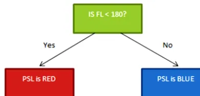
Figure 1.An example of a small decision tree.
considered here since they rely on the user to input the num-ber of clusters, which in an ambient situation is unlikely to be known prior to the analysis. There are seven available link-ages in the Fastcluster package (Müllner, 2013, 2011): single (closest point), complete (furthest point), average (average distance), weighted (weighted average distance), ward (min-imisation of variance), centroid (difference between means) and median (differences between medians). Prior to this anal-ysis we used thezscore to standardise the data.
2.2 Decision trees and ensemble methods
When using decision trees, data are split by sorting the data by each variable and using a metric to find the best place to split. An example of a decision tree is given in Fig. 1. In our example there are two groups, blue particles and red parti-cles, and the variable we use to split them is a measurement of fluorescent intensity of the particle. In reality the tree will be much more complicated with many more branches.
To construct the decision tree we consider all possible splits within the data. For example if we had three particles with fluorescent intensity (FL) of 180, 300 and 1400 arbi-trary units, we would consider all possible splits to determine the best split for the first branch. For three particles there would be three possible cases for the first branch: FL>180, FL>300 and FL>1400. Each split then will be evaluated using a criterion to determine how effective the split is to dis-tinguish between the different groups. All of the other vari-ables are then considered in the same fashion and the most effective split for the first branch in the data is selected. The process is then repeated to split the data multiple times, cre-ating a larger tree with many branches. In the case of our example we would have a tree with two splits. When clas-sifying a new particle we simply start at the top of the tree, evaluating the criteria until a conclusion about the particle is made.
Multiple decision trees can be combined to create ensem-ble classifiers. These classifiers often achieve improvements in one of two ways. Firstly, classifiers such as bagging and random forests take samples of the data and the variables, which are used to produce different decision trees, each ca-pable of classifying a particle. Averaging the classifications made by each tree is then thought to give an overall better
re-sult. An alternative approach used by the AdaBoost classifier and the gradient boosting classifier is to begin by weighting all the data equally and over several iterations have decision trees focus on the parts of the data that are being misclas-sified most often. This can yield an improvement over the single decision tree as the classifier is modified to correct the mistakes that it is making. These ensemble methods could be theoretically used with other classifiers but the simplicity and speed of the decision trees mean that they are most often used. We give further details of the ensemble methods below. Bagging (Breiman, 1996) is where multiple samples of the data are taken and a different tree is fitted to each of the sam-ples. The samples taken are bootstrap samples, a common statistical technique used to create multiple data sets from one set of data. This can be thought as putting all the sam-ples into a bag, taking out one sample at a time and putting it back into the bag. This is repeated until a new data set which is the same size as the original is obtained. Some samples will have been selected more than once from the bag and others may not get selected at all. This gives a subtly different data set. This can be repeated multiple times in order to create multiple versions of the data set. From each of the samples a decision tree is constructed and the results from the dif-ferent trees are then averaged to give an overall result. The rationale behind the method is that slight differences in the different versions of the data set will produce different trees and in averaging the results we will get a better estimation of which group the particle belongs to.
Bagging is extended to “random forests” in Breiman (2001). Instead of selecting the best split when constructing any particular tree, a random subset of variables is chosen to build the tree. It is hypothesised that using only a subset of the variables will produce trees that are more independent and thus the improvement from averaging can be larger. Ran-dom forests are generally considered to perform better than bagging; hence we do not consider bagging in our analysis.
An alternative method for combining decision trees into an ensemble classifier is AdaBoost (Freund and Schapire, 1995). Here weights are assigned to each of the particles and very small decision trees are fitted to the data. Performance is evaluated using a loss function (exponential loss function) and the data are re-weighted to focus on particles that are being misclassified most often. Gradient boosting is a gen-eralisation of the AdaBoost algorithm to allow for different loss functions.
2.3 Gaussian-based methods
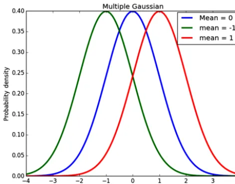
An alternative approach to solve the classification problem is to fit multivariate normal distributions to each of the groups within the training data. This distribution is a generalisation of the normal distribution for one variable and depends on the means and covariance of the different variables.
Figure 2.An example of three fitted normal distributions.
no requirements on the covariance this results in QDA. The assumption that each of the groups vary equally results in LDA and finally making the assumption that each of the vari-ables are independent of each other results in Gaussian naïve Bayesian.
Once the normal distributions are fitted we can classify new particles by calculating the probability that the particle comes from each of the groups and assigning it to the group that it is most likely to have come from.
As an example, in Fig. 2 we have plotted normal distri-butions for three groups. If we were to observe a value of x=0 then the particle would be assigned to the blue group as the probability that the particle comes from the blue group is higher than that for the red and for the green.
2.4 K-nearest neighbour classification (KNN)
This method does not require a training step; instead, to clas-sify a previously unseen particle the particle is compared to each of the particles in the training set and the k-nearest neighbours in the training set to the previously unseen par-ticle are recorded. The previously unseen parpar-ticle is then at-tributed to the same group as the majority of its nearest neigh-bours. This method can be regarded as recognition rather than learning as it classifies a particle simply on how simi-lar it is to particles that it has seen in the training data.
2.5 Support vector machines
A practical guide to support vector classification is given in Hsu et al. (2003). The method transforms the data to a higher-dimensional space and then splits the data using a linear deci-sion function (Cortes and Vapnik, 1995). In two dimendeci-sions this would be a line, in three a plane, etc. In two dimensions, points to one side of the line are classified as coming from one group; points on the other side of the line are classified
as coming from the other group. Points to either side of the line correspond to positive and negative values of the deci-sion function respectively. The line is selected on the basis of how well it splits the data without giving too much prece-dence to outliers.
In order to generalise this methods to multiple groups there are two methods: one-vs.-rest and one-vs.-one. One-vs.-rest involves fitting a support vector machine for each of the groups against the rest of the groups and then attributing new particles to the group with the highest value of the decision function. One-vs.-one fits a classifier to each pair of groups and then uses a voting scheme to attribute previously unseen particles to a group. LinearSVC (linear support vector classi-fication) uses the one-vs.-rest strategy whereas SVC (support vector classification) uses the one-vs.-one strategy.
How the data are transformed to a higher-dimensional space is dependent on the kernel chosen. There are two im-plementations within scikit-learn (Pedregosa et al., 2011) that can be used for support vector machines: SVC and Lin-earSVC. The former allows many different kernels, whereas the latter is a faster version of the first but is limited to the linear kernel only. We test SVC using the RBF (radial basis function) kernel and use linearSVC for the linear kernel.
The SVC implementation has parametersγ andC. Since γis a specific parameter for the RBF kernel, LinearSVC only requires the input of the value ofC. Using a sample of 10 % of the data, we test the values ofC equal to 1, 10, 100 and 1000 and in the case of the SVC function we test all pos-sible combinations ofC withγ equal to 0, 1, 10, 100 and 1000. The values are selected to test a wide range of possi-ble values of each of the parameters to allow for appropriate values to be selected. In future, it might be possible to get better performance by either conducting this initial parame-ter selection on a larger sample of the data or testing more values, but within the scope of this paper we are intending to select parameters that perform fairly well, which should give us an appropriate estimation on the effectiveness of the method. The values which perform best are used with the five-fold cross validation to form our final result.
2.6 Artificial neural networks
Artificial neural networks are statistical models inspired loosely by neurons within the brain. They have been shown to be particularly effective for complex problems such as digit classification (LeCun et al., 1998). As with support vector machines, it is recommended that each of the variables are standardised using thezscore to ensure that each of the vari-ables are given equal weighting when training the neural net-work.
hid-den units, or neurons. Synapses connect the input layer to the hidden layer(s) and from the hidden layer(s) to the out-put layer. The synapses have a simple job of multiplying the input value by a weight and producing an output value. The neurons will sum the outputs of the synapses and apply an activation function. Finally we have an output layer. For our data this will be the classification of the particle, e.g. bacteria or blue PSL. For this paper we experimented with using one hidden layer with 10 hidden units and two hidden layers with 500 and 10 units respectively.
Initially the weights in the network are set randomly us-ing a normal distribution with mean 0 and standard deviation of 0.01. Since the weights have been initialised randomly at this point the network will perform very poorly. However, as data are passed through the network, the weights are adjusted to minimise a loss function. Once training is completed the weights should better reflect the learning task and then the network is used to classify the testing set.
The scikit-learn package does not currently contain an im-plementation for neural networks but is undergoing develop-ment and will likely do so in the future. For this paper we elect to use pycaffe (Jia et al., 2014), which is a fast package for implementing a variety of different neural networks.
3 Instrumentation
The Multiparameter Bioaerosol Spectrometer (MBS) is a de-velopment of the Wideband Integrated Bioaerosol Spectrom-eter (WIBS) technology developed by the University of Hert-fordshire (Kaye et al., 2005). Both instruments are designed to acquire data relating to the size, shape and intrinsic fluo-rescence of individual airborne particles and use these data to detect and potentially classify those particles that are of biological origin. However, whereas the WIBS instrument records particle fluorescence over just two wavebands, ap-proximately 310–400 and 420–650 nm (corresponding to the maximum emissions from tryptophan and NADH), the MBS records the fluorescence over eight equal wavelength bands from approximately 310 to 640 nm. This is likely to provide better discrimination between biological particles and “in-terferent” non-biological particles that may exhibit similar fluorescence properties. Similarly, while WIBS uses a sim-ple 4 pixel detector to assess particle shape from the parti-cle’s spatial light scattering pattern (Kaye et al., 1996; Kaye, 1998), the MBS uses an arrangement of two 512 pixel CMOS detector arrays to record high-resolution details of the parti-cle’s spatial light scattering pattern, allowing both the macro-scopic shape of the particle and potentially particle surface characteristics to be determined. Again, this can enhance the prospects of particle classification and reduces false-positive bio-particle detection. The key elements of the MBS are shown in Fig. 3.
The MBS draws ambient aerosol through an inlet tube at a rate of approximately 1.5 L min−1. Part of this flow is
fil-tered and used both as a “bleed” flow (to maintain cleanliness of the inner optical chamber) and as a “sheath” flow which surrounds and constrains the remaining “sample” flow. Parti-cles carried in the remaining 300 mL min−1sample flow are forced to pass in single file through the sensing volume, de-fined by the intersection between the particle detection laser beam (see below) and the sample airflow column.
Each particle carried in the sample airflow is initially de-tected by a low-power laser beam (12 mW at 635 nm). The light scattered from the laser pulse is collected by the lens assembly shown at the upper-right of Fig. 3 and a small pro-portion of the light is directed by a pellicle beam splitter to the photodiode trigger detector. The voltage output pulse of this detector is proportional to the intensity of light falling on it and is used to size the particle. The trigger signal also initi-ates the firing of a second, high-power, pulsed laser (250 mW at 637 nm) that irradiates the particle with sufficient inten-sity to allow elements of the particle’s spatial light scatter-ing pattern, which relates to particle morphology and orien-tation (Kaye, 1998), to be captured by the arrangement of two CMOS linear detector arrays.
About 10 µs after particle detection, the UV xenon source illuminates the particle for approximately 1 µs with an in-tense UV pulse at 280 nm wavelength. The resulting fluo-rescent light from the particle is collected by two spherical mirrors and directed through to the spectrometer optics. The fluorescence spectrum, covering 310–650 nm, is recorded by the eight-channel photomultiplier tube and the information is digitised and recorded by the electronics control unit. The particle then passes out of the chamber and the system is re-armed. The total measurement process takes 30 µs. Despite the fact that the system is capable of counting particles at a rate greater than 1000 per second, the limiting factor is the xenon recharge time (approximately 5 ms), which reduces the data acquisition rate to approximately 100 particles a sec-ond (this correspsec-onds to measuring all particles to a concen-tration of 2×10⁴particles L−1.
Figure 3.Schematic diagram of the Multiparameter Bioaerosol Spectrometer.
Figure 4.Typical fluorescence spectral data (left) and spatial light scattering data (right) recorded from a single aerosol particle by the MBS instrument.
4 Data
In order to evaluate the performance of the various different methods we use two different data sets. For each of the data sets we have included a parallel coordinate plot to allow the reader to see on average how each of the groups differ in their fluorescent intensity and size (see Figs. 5 and 6).
4.1 Polystyrene latex spheres
From Fig. 5 it should be clear that the PSLs should be highly separable by eye. This data set provides a benchmark of the simplest separation task. We would expect a good classifica-tion technique to perform well with this data set.
Figure 5.Average fluorescent intensity given in arbitrary units (AU) for the eight fluorescent channels and the size given in micrometres for the PSL data.
Figure 6.Average fluorescent intensity given in arbitrary units (AU) for the eight fluorescent channels and the size given in micrometres for the laboratory data. The fluorescent signatures for the paper mul-berry sample are not included in the figure as the particles are much larger and more fluorescent than the remaining samples and their inclusion would cause the graph to be uninterpretable.
in which hierarchical agglomerative clustering was shown to effectively discriminate particles of this kind.
4.2 Laboratory data
The laboratory data used here are an attempt to provide chal-lenging aerosol particles that are more representative of those occurring naturally in the environment and between which a bioaerosol sensor will need to discriminate. These data con-tain examples of various different fungal spores, pollen, bac-teria and non-fluorescent mabac-terial that might be found within ambient data.
The materials listed in Table 2 were aerosolised into a large, clean HEPA filtered containment chamber (incorpo-rating a recirculation fan), from which the aerosol inlet of
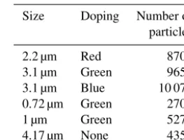
Table 1.Sample sizes for PSLs.
Size Doping Number of particles
2.2 µm Red 8704 3.1 µm Green 9651 3.1 µm Blue 10 076 0.72 µm Green 2702 1 µm Green 5274 4.17 µm None 4351
the MBS sensor drew the measurement samples. Liquids and suspensions were nebulised using a medical mini-nebuliser (e.g. Hudson RCI Micro-Mist nebuliser), while the dry mate-rials were aerosolised directly from small quantities of pow-der using a filtered compressed air jet.
TheBacillus atrophaeus (BG) andE. colibacteria were generated from suspensions in L-broth growth media, so these aerosols also contain particles of L-broth. Some of the BG spores were also washed before use (by filtering the sus-pension and re-suspending the spores in distilled water) to obtain relatively clean aerosolised spores.
Measurements of a rye grass pollen sample were taken but only consisted of approximately 50 particles, substantially less than the other samples, and so were removed.
The remaining particles were split into four broad groups: bacteria, fungal spores, pollen and non-fluorescent material. Details of the sample sizes and group classifications are given in Table 2.
5 Results
5.1 General results
After being split into training and testing data, as outlined in Sect. 2, the proportion of the testing data correctly classified for each of the supervised methods for each of the data sets is given in Figs. 7 and 8. In the case of the unsupervised method (HCA) it was not necessary to split the data into training and testing sets. Instead we applied the algorithm with all seven available linkages to all the particles. The results for which, for ease of comparison, are also given in Figs. 7 and 8.
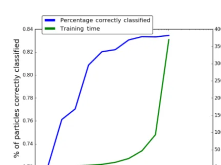
We have also provided a subset of our time results. In Fig. 9 we have the training and testing times for the super-vised methods and the full time taken for the HCA for the full mixed PSL data. The timings for the reduced data set and for the laboratory-generated aerosol are omitted as they show similar patterns. Note in particular that our training set is four times bigger than our testing set since we have used five-fold cross validation (see Sect. 2).
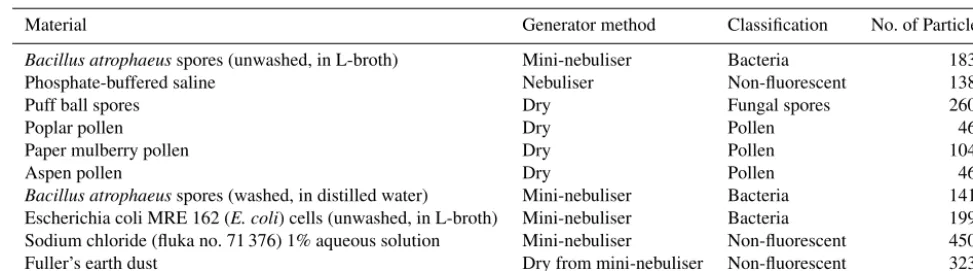
Table 2.Classification, generator method and sample size of different samples from the laboratory data.
Material Generator method Classification No. of Particles
Bacillus atrophaeusspores (unwashed, in L-broth) Mini-nebuliser Bacteria 1831 Phosphate-buffered saline Nebuliser Non-fluorescent 1388
Puff ball spores Dry Fungal spores 2607
Poplar pollen Dry Pollen 469
Paper mulberry pollen Dry Pollen 1041
Aspen pollen Dry Pollen 466
Bacillus atrophaeusspores (washed, in distilled water) Mini-nebuliser Bacteria 1417 Escherichia coli MRE 162 (E. coli) cells (unwashed, in L-broth) Mini-nebuliser Bacteria 1991 Sodium chloride (fluka no. 71 376) 1% aqueous solution Mini-nebuliser Non-fluorescent 4502 Fuller’s earth dust Dry from mini-nebuliser Non-fluorescent 3238
Figure 7.Performance of the different methods in terms of particles correctly classified for the mixed PSLs. The results on the left are for the full data set and on the right are the results for the reduced data set. Full names of each of the methods are given in Table 3.
achieved by using all the data in the HCA analysis (includ-ing both saturated and non-fluorescent material), for the lab-oratory data, it was beneficial to remove saturated and non-fluorescent material before conducting HCA analysis. Pre-filtering was not applied to the supervised methods as ex-plained in the Sect. 2. Only the best results are listed in Figs. 7 and 8; i.e. for the PSLs the results listed are from when all the particles were included and for the laboratory data the results obtained from the removal of non-fluorescent and fluorescent material are listed.
With the inclusion of the 1024 shape measurements we have a high-dimensional data set, without we have a rela-tively low-dimensional data set (nine dimensions). To give a good indication of the robustness of each algorithm to di-mensionality as well as to ascertain whether the additional
Figure 8.Performance of the different methods in terms of particles correctly classified and a breakdown of the errors for the laboratory-generated aerosols. The results on the left are for the full data set and on the right are the results for the reduced data set. Full names of each of the methods are given in Table 3.
shape information yields any benefit, we provide results for both the full data set (1024 shape measurements, 8 fluores-cent measurements and 1 size measurement) and the reduced data set (eight fluorescent measurements and one size mea-surement).
In Fig. 5 we see that the dye-doped PSLs should be highly separable by eye whereas in Fig. 6 it appears the laboratory data would present more of a challenge to the different al-gorithms. This is demonstrated also in our results where the percentage of data correctly classified for the laboratory data is in general much lower than that of the PSLs.
Table 3.Key for the shortened names for the different methods given in the figures.
Key Method Subsection Key Method Subsection
SIN HCA (single linkage) 2.1 RF Random forest 2.2 COM HCA (complete linkage) 2.1 LDA Linear discriminant analysis 2.3 AVE HCA (average linkage) 2.1 QDA Quadratic discriminant analysis 2.3 WEI HCA (weighted linkage) 2.1 GNB Gaussian naïve Bayesian 2.3 WAR HCA (ward linkage) 2.1 KNN KNearest-neighbour 2.4 CEN HCA (centroid linkage) 2.1 SVC Support vector classification 2.5 MED HCA (median linkage) 2.1 LSVC Linear support vector classification 2.5 DT Decision tree 2.2 NN1 Neural network – 1 Layer 2.6 GB Gradient boosting 2.2 NN2 Neural network – 2 Layers 2.7
ADA AdaBoost 2.2
Figure 9.Performance of the different methods in terms of the time it takes for the method to train and test for the mixed PSLs.
the laboratory-generated aerosol. However, since we have already placed the non-fluorescent material and saturated material into groups on their own prior to analysis for the laboratory-generated aerosol, we see better performance for the laboratory data compared to the PSLs in this case. For the reduced data, however, we can yield generally good perfor-mance for the PSLs using the Ward linkage, but for the lab-oratory data the performance is generally poorer compared with the supervised methods regardless of whether the shape information is included.
Should these methods be applied to real-time applications, we would expect the testing data to contain much larger num-ber of particles compared to the training data. For example, we could collect between 104and 105particles of laboratory data for training. However, over the space of several months in an ambient contain we might collect 106particles or more. It is for this reason we conclude that methods such as the ensemble methods and neural networks offer distinct advan-tages over HCA. For HCA the time requirements increase at a much faster rate than the number of particles (Müllner,
2011). In other words a doubling in the amount of data will result in more than a doubling in the amount of time required. A similar behaviour is true for the full support vector ma-chines classifier.
The behaviour of the neural networks and the ensemble methods is much more desirable. While the training times are relatively large compared to other methods, once the model is fitted the testing time requirements are under a second for several thousand particles, which is much faster than the maximum count rate of the instrument.
Some of the methods, in particular the cluster analysis and the QDA perform poorer or equally as poor when the shape information is included. This is a reflection of the methods’ ability to utilise high-dimensional data effectively rather on the instrument itself. In the case of HCA we would suggest that further research needs to be conducted in order to re-duce the dimensionality of the data without losing informa-tion from the shape channels before using this method for the MBS. For QDA, the difficulty is in approximating the covari-ance matrix when the number of samples is less or similar to the number of dimensions. We would hence expect this method to perform better as larger samples are collected.
Decision trees and ensemble methods appear to be rela-tively robust to the introduction of the higher-dimensional data. This is to be expected since most of the methods un-dergo some kind of variable selection. Gradient boosting, however, does seem to offer improvements on the AdaBoost algorithm and random forests seem to improve on decision trees as is suggested in the literature.
Overall the best performing method was LDA for the PSLs and for laboratory-generated aerosols the gradient boost-ing algorithm performed better. Note, however, that gradient boosting only classified 0.23 % less of the data correctly than LDA in the case of the PSLs data so overall our results indi-cate that gradient boosting is the best performing algorithm.
with additional layers, that this should be done using a graph-ics processing unit (GPU) which could offer significant gains in the amount of time required to train the network. This is a benefit over the gradient boosting algorithm, where it is far less clear how the algorithm might be parallelised.
In contrast, neural networks are very difficult for the user to tailor to achieve good performance. The results presented are achieved after a lot of experimentation, especially in terms of the learning rate. A learning rate that is too high often will overshoot a minimum for the loss function and a learning rate that is too low will fail to reach a minimum at all. Overfitting, where the model fits very well for the train-ing data but does not generalise well for the testtrain-ing data, is also an issue. Overfitting seems not to be a problem for the gradient boosting algorithm, which also did not require any parameter selection by the user.
5.2 Further analysis for the gradient boosting algorithm
Due to the number of methods tested it is not practical to pro-vide detailed information on all methods; instead we propro-vide additional analysis for the gradient boosting algorithm which we found to offer, in general, better performance than the other methods. In particular we provide a further breakdown of the error term in Sect. 5.2.1. In Sect. 5.2.2 we split the lab-oratory data into individual samples and repeat the analysis. Finally in Sect. 5.2.3, we investigate the importance of the variables and the implication of removal of lesser important variables.
5.2.1 Breakdown of error
We can see in Figs. 7 and 8 that even for gradient boost-ing we still have a significant error in the classification rate. We therefore have elected to further break this error down into the different classes in Table 4. What we can see is that not only is a large proportion of the error due to fluorescent material being misclassified as non-fluorescent but the fun-gal spore sample is a particularly large source of error. How-ever, amongst the material that was classified as fluorescent misclassification between the fluorescent classes is relatively small; e.g. only 67 fungal spores have been misclassified as bacteria.
As further samples are collected, especially in the case of fungal spores, we would hope these errors will start to de-crease. However, an ongoing issue with the technique ap-pears to be that a significant amount of particles within the fluorescent samples are weakly fluorescent and hence are dif-ficult to classify correctly.
5.2.2 Classification of individual species
Our analysis in Sect. 5.1 only considers the broad biological classes: bacteria, fungal spores and pollen. In this subsection we enhance this analysis to split the bacteria into the three
Table 4.Breakdown of error for the gradient boosting algorithm on the full data set. For example, in the third row and first column we can see 31 particles of the bacteria sampled were classified as fungal spores.
Bacteria Fungal Pollen Non-spores fluorescent
Bacteria 4637 67 66 174
Fungal spores 24 993 72 214
Pollen 31 58 1382 61
Non-fluorescent 547 1489 456 8679
individual samples (i) washed BG spores, (ii) unwashed BG spores and (iii) unwashedE. coli. Similarly the pollen sam-ples are also split up into (i) poplar pollen, (ii) aspen pollen and (iii) paper mulberry.
From Table 5 we can see that in the case of the bacterial samples we can effectively differentiate the washed sample from the unwashed samples. Distinguishing between theE. coliand the BG spores is also possible but with lesser suc-cess. It is entirely possible to distinguish between the paper mulberry and the other pollen samples but not between the aspen and poplar pollen sample. This is to be expected as the paper mulberry particles are significantly different from the aspen and poplar pollen samples, but the differences between the aspen and poplar pollen are very small.
Across all samples, excluding the particles which are in-correctly classified as non-fluorescent, when particles are misclassified they are most likely to be misclassified as a dif-ferent sample from the same broad biological classes (bacte-ria, fungal spores and pollen). For example for the BG spores (w) sample, excluding the material that is misclassified as non-fluorescent, the largest misclassification is from particles being misclassified asE. coli(uw), which is still bacteria.
5.2.3 Variable importance
Since the instrument presented offers more information than the WIBS for example, it seems necessary to evaluate which of the variables presented offers the most information and how much of an impact removing lesser important variables has, on both time and the percentage of particles correctly classified.
It is possible to evaluate the performance of variables us-ing the ensemble methods, e.g. gradient boostus-ing. This is be-cause each of the decision trees that come together to form the ensemble identifies which variables are best to split dur-ing the traindur-ing stage. It is therefore possible to find out how often each of the variables are used to produce a split and this will give an indication of how important each of the variables are.
Table 5.Further breakdown of error for the gradient boosting algorithm on the full data set. The abbreviations (w) and (uw) are used for washed and unwashed samples respectively.
BG spores BG spores E. coli Puffballs Paper Aspen Poplar Non-(w) (uw) (uw) mulberry pollen pollen fluorescent
BG spores (w) 1127 12 71 5 0 4 2 39
BG spores (uw) 4 1373 197 19 6 9 16 27
E. coli(uw) 79 227 1385 20 6 8 15 41
Puffballs 3 16 13 1082 10 35 62 254
Paper mulberry 0 5 3 15 998 2 2 11
Aspen pollen 2 7 3 13 2 109 65 22
Poplar pollen 1 8 2 23 1 50 68 20
Non-fluorescent 201 183 317 1430 18 249 239 8714
and train the algorithm on the subset of the data and record the importance of each of the variables. In Fig. 10 we show the importance of the variables for the full data, bacteria vs. fungal spores (pollen removed), bacteria vs. pollen (fungal spores removed) and finally fungal spores vs. pollen (bacte-ria removed). The top three most important va(bacte-riables always contained a selection of four different variables, so we pro-vide the importance for these four variables in Fig. 10.
Finally, we remove all but the top 512, 256, 128, . . . , 2 variables and repeat the analysis. The total time required and the percentage of particles classified correctly are given in Fig. 11.
What we can see from our analysis is that for the data set with none of the broad biological classes (bacteria, pollen and fungal spores) removed the most important variable is the Size followed by the third fluorescent channel. For the remaining subsets of the data tested the most important vari-ables are a fluorescent variable followed by the size. From Fig. 11, however, we can see that four variables alone, while the most important, are not sufficient to maintain the results possible with the full data set. Instead, reduction in the num-ber of variables does necessarily lead to a reduction in per-formance in someway. Nonetheless the decrease from 1024 variables to 128 produces a very small decrease in perfor-mance and hence a smaller shape detector may be sufficient.
6 Conclusions
Ultraviolet light-induced fluorescence (UV-LIF) is becoming a widely used and accepted method for collecting fluores-cent signatures for bioaerosols. However, the applicability of the method has yet to be demonstrated for routine real-time monitoring and reporting applications for airborne biological particles. In this paper we have combined the well-developed and researched field of machine learning with the applica-tion of identifying atmospheric aerosol. We have demon-strated that previously used unsupervised methods may not be best at discriminating between aerosol using single parti-cle broadband UV-LIF spectrometers and using the MBS we
Figure 10.Variable importance for the different subsets of the data.
Figure 11.Variable importance for the different subsets of the data.
have identified the gradient boosting classifier as a possible supervised alternative.
of bioaerosol. Cluster analysis, while working well for the reduced data set for PSLs, seems to struggle for the laboratory-generated aerosol and when applied to the higher-dimensional data set, so we suggest that more research for this method is required before it could be reasonably used on ambient data collected using the MBS. For the Gaussian methods it seems that the methods work reasonably well for the PSLs, but we believe there are better alternatives when discriminating between atmospheric aerosol.
For thek-nearest neighbours method we believe that a lim-iting factor is in the time it takes for the method to classify the testing data. Similarly, while the full support vector ma-chine performs very well, the time requirements would be inappropriate when larger samples are collected. Conversely, while the linear version of the support vector machine per-forms much faster, it is at the cost of performance, so we sug-gest that support vector machines not be used for this task.
Overall, the method we suggest for classification of at-mospheric aerosol is the gradient boosting algorithm which produces the best results with limited user input but has the drawback that it cannot easily be parallelised. Another possi-ble alternative in the future, once more research is conduced, is the neural network, which can be easily ported to a GPU for substantial speedup in training but requires a much larger input for the user and produces slightly worse results com-pared to the gradient boosting algorithm.
From our further analysis of the gradient boosting algo-rithm we also see that a disadvantage for the data we have collected is in the sample of fungal spores, which is often misclassified as non-fluorescent since a good proportion of the particles is weakly fluorescent. We believe this issue can be circumvented with collection of a wider range of fungal spore samples in the future. Also, we see that for the MBS we have reasonable success in discriminating between single bacterial samples.
Finally we realise that performance can be maintained while removing a reasonable number of the lesser important variables, leading us to conclude that a smaller shape detec-tor may be sufficient.
Since these supervised learning algorithms have yet to be applied to the data produced using the WIBS it is not cur-rently possible to draw any clear conclusions as to the per-formance of the MBS versus the WIBS. Instead the authors suggest that to provide direct comparison, further research needs to be undertaken whereby both instruments are used for identical samples.
7 Data availability
The data used to formulate the results in the pa-per can be provided upon request by contacting the first author, using the correspondence e-mail address ([email protected]).
Acknowledgements. Simon Ruske is funded by a NERC grant (NE/L002469/1) as part of the Manchester–Liverpool Doctoral Training Partnership. The MBS instrument was funded by the NERC research grant, NE/K006002/1 “Ice Nucleation Process Investigation and Quantification”.
Edited by: F. Pope
Reviewed by: D. Baumgardner and one anonymous referee
References
Breiman, L.: Bagging predictors, Mach. Learn., 24, 123–140, 1996. Breiman, L.: Random forests, Mach. Learn., 45, 5–32, 2001. Cortes, C. and Vapnik, V.: Support-vector networks, Mach. Learn.,
20, 273–297, 1995.
Crawford, I., Bower, K. N., Choularton, T. W., Dearden, C., Crosier, J., Westbrook, C., Capes, G., Coe, H., Connolly, P. J., Dorsey, J. R., Gallagher, M. W., Williams, P., Trembath, J., Cui, Z., and Blyth, A.: Ice formation and development in aged, wintertime cu-mulus over the UK: observations and modelling, Atmos. Chem. Phys., 12, 4963–4985, doi:10.5194/acp-12-4963-2012, 2012. Crawford, I., Robinson, N. H., Flynn, M. J., Foot, V. E., Gallagher,
M. W., Huffman, J. A., Stanley, W. R., and Kaye, P. H.: Char-acterisation of bioaerosol emissions from a Colorado pine for-est: results from the BEACHON-RoMBAS experiment, Atmos. Chem. Phys., 14, 8559–8578, doi:10.5194/acp-14-8559-2014, 2014.
Crawford, I., Ruske, S., Topping, D. O., and Gallagher, M. W.: Eval-uation of hierarchical agglomerative cluster analysis methods for discrimination of primary biological aerosol, Atmos. Meas. Tech., 8, 4979–4991, doi:10.5194/amt-8-4979-2015, 2015. Cziczo, D. J., Froyd, K. D., Hoose, C., Jensen, E. J., Diao, M.,
Zondlo, M. A., Smith, J. B., Twohy, C. H., and Murphy, D. M.: Clarifying the dominant sources and mechanisms of cirrus cloud formation, Science, 340, 1320–1324, 2013.
Freund, Y. and Schapire, R. E.: A desicion-theoretic generalization of on-line learning and an application to boosting, in: Computa-tional learning theory, Springer, 23–37, 1995.
Gurian-Sherman, D. and Lindow, S. E.: Bacterial ice nucleation: significance and molecular basis, FASEB J., 7, 1338–1343, 1993. Hader, J. D., Wright, T. P., and Petters, M. D.: Contribution of pollen to atmospheric ice nuclei concentrations, Atmos. Chem. Phys., 14, 5433–5449, doi:10.5194/acp-14-5433-2014, 2014.
Healy, D. A., Huffman, J. A., O’Connor, D. J., Pöhlker, C., Pöschl, U., and Sodeau, J. R.: Ambient measurements of bio-logical aerosol particles near Killarney, Ireland: a comparison between real-time fluorescence and microscopy techniques, At-mos. Chem. Phys., 14, 8055–8069, doi:10.5194/acp-14-8055-2014, 2014.
Herich, H., Gianini, M., Piot, C., Moˇcnik, G., Jaffrezo, J.-L., Be-sombes, J.-L., Prévôt, A., and Hueglin, C.: Overview of the im-pact of wood burning emissions on carbonaceous aerosols and PM in large parts of the Alpine region, Atmos. Environ., 89, 64– 75, 2014.
Hoose, C. and Möhler, O.: Heterogeneous ice nucleation on atmo-spheric aerosols: a review of results from laboratory experiments, Atmos. Chem. Phys., 12, 9817–9854, doi:10.5194/acp-12-9817-2012, 2012.
Hsu, C., Chang, C., and Lin, C.: A practical guide to support vector classification, Department of Computer Science and Information Engineering, National Taiwan University, Taipei, Taiwan, 2003. Huffman, J. A., Prenni, A. J., DeMott, P. J., Pöhlker, C., Mason, R.
H., Robinson, N. H., Fröhlich-Nowoisky, J., Tobo, Y., Després, V. R., Garcia, E., Gochis, D. J., Harris, E., Müller-Germann, I., Ruzene, C., Schmer, B., Sinha, B., Day, D. A., Andreae, M. O., Jimenez, J. L., Gallagher, M., Kreidenweis, S. M., Bertram, A. K., and Pöschl, U.: High concentrations of biological aerosol par-ticles and ice nuclei during and after rain, Atmos. Chem. Phys., 13, 6151–6164, doi:10.5194/acp-13-6151-2013, 2013.
Hummel, M., Hoose, C., Gallagher, M., Healy, D. A., Huffman, J. A., O’Connor, D., Pöschl, U., Pöhlker, C., Robinson, N. H., Schnaiter, M., Sodeau, J. R., Stengel, M., Toprak, E., and Vogel, H.: Regional-scale simulations of fungal spore aerosols using an emission parameterization adapted to local measurements of flu-orescent biological aerosol particles, Atmos. Chem. Phys., 15, 6127–6146, doi:10.5194/acp-15-6127-2015, 2015.
Jacobson, M. Z. and Streets, D. G.: Influence of future an-thropogenic emissions on climate, natural emissions, and air quality, J. Geophys. Res.-Atmos., 114, D08118, doi:10.1029/2008JD011476, 2009.
Jia, Y., Shelhamer, E., Donahue, J., Karayev, S., Long, J., Girshick, R., Guadarrama, S., and Darrell, T.: Caffe: Convolutional Ar-chitecture for Fast Feature Embedding, Proceedings of the 22nd ACM international conference on Multimedia, Orlando, Florida, USA, 3–7 November 2014, 675–678, 2014.
Joly, M., Attard, E., Sancelme, M., Deguillaume, L., Guilbaud, C., Morris, C. E., Amato, P., and Delort, A.-M.: Ice nucleation ac-tivity of bacteria isolated from cloud water, Atmos. Environ., 70, 392–400, 2013.
Kaye, P., Stanley, W., Hirst, E., Foot, E., Baxter, K., and Barrington, S.: Single particle multichannel bio-aerosol fluorescence sensor, Opt. Express, 13, 3583–3593, 2005.
Kaye, P. H.: Spatial light-scattering analysis as a means of charac-terizing and classifying non-spherical particles, Meas. Sci. Tech-nol., 9, 141–149, 1998.
Kaye, P. H., Alexander-Buckley, K., Hirst, E., Saunders, S., and Clark, J.: A real-time monitoring system for airborne particle shape and size analysis, J. Geophys. Res.-Atmos., 101, 19215– 19221, 1996.
Kennedy, R. and Smith, M.: Effects of aeroallergens on human health under climate change, in: Health Effects of Climate Change in the UK 2012, edited by: Vardoulakis, S. and Heavi-side, C., 83–96, 2012.
LeCun, Y., Bottou, L., Bengio, Y., and Haffner, P.: Gradient-based learning applied to document recognition, Proceedings of the IEEE, 86, 2278–2324, 1998.
Möhler, O., DeMott, P. J., Vali, G., and Levin, Z.: Microbiology and atmospheric processes: the role of biological particles in cloud physics, Biogeosciences, 4, 1059–1071, doi:10.5194/bg-4-1059-2007, 2007.
Morris, C. E., Conen, F., Alex Huffman, J., Phillips, V., Pöschl, U., and Sands, D. C.: Bioprecipitation: a feedback cycle linking Earth history, ecosystem dynamics and land use through biolog-ical ice nucleators in the atmosphere, Glob. Change Biol., 20, 341–351, 2014.
Müllner, D.: Modern hierarchical, agglomerative clustering algo-rithms, available at: https://arxiv.org/abs/1109.2378, 2011. Müllner, D.: fastcluster: Fast hierarchical, agglomerative clustering
routines for R and Python, J. Stat. Softw., 53, 1–18, 2013. Pedregosa, F., Varoquaux, G., Gramfort, A., Michel, V., Thirion,
B., Grisel, O., Blondel, M., Prettenhofer, P., Weiss, R., Dubourg, V., Vanderplas, J., Passos, A., Cournapeau, D., Brucher, M., Per-rot, M., and Duchesnay, E.: Scikit-learn: Machine Learning in Python, J. Mach. Learn. Res., 12, 2825–2830, 2011.
Prenni, A., Tobo, Y., Garcia, E., DeMott, P., Huffman, J., Mc-Cluskey, C., Kreidenweis, S., Prenni, J., Pöhlker, C., and Pöschl, U.: The impact of rain on ice nuclei populations at a forested site in Colorado, Geophys. Res. Lett., 40, 227–231, 2013.
Robinson, N. H., Allan, J. D., Huffman, J. A., Kaye, P. H., Foot, V. E., and Gallagher, M.: Cluster analysis of WIBS single-particle bioaerosol data, Atmos. Meas. Tech., 6, 337–347, doi:10.5194/amt-6-337-2013, 2013.
Schumacher, C. J., Pöhlker, C., Aalto, P., Hiltunen, V., Petäjä, T., Kulmala, M., Pöschl, U., and Huffman, J. A.: Seasonal cycles of fluorescent biological aerosol particles in boreal and semi-arid forests of Finland and Colorado, Atmos. Chem. Phys., 13, 11987–12001, doi:10.5194/acp-13-11987-2013, 2013.
Spracklen, D. V. and Heald, C. L.: The contribution of fungal spores and bacteria to regional and global aerosol number and ice nucle-ation immersion freezing rates, Atmos. Chem. Phys., 14, 9051– 9059, doi:10.5194/acp-14-9051-2014, 2014.
Tobo, Y., Prenni, A. J., DeMott, P. J., Huffman, J. A., McCluskey, C. S., Tian, G., Pöhlker, C., Pöschl, U., and Kreidenweis, S. M.: Biological aerosol particles as a key determinant of ice nuclei populations in a forest ecosystem, J. Geophys. Res.-Atmos., 118, 10100–10110, doi:10.1002/jgrd.50801, 2013.