www.ocean-sci.net/8/903/2012/ doi:10.5194/os-8-903-2012
© Author(s) 2012. CC Attribution 3.0 License.
Ocean Science
Modelling temperature and salinity in Liverpool Bay and the Irish
Sea: sensitivity to model type and surface forcing
C. K. O’Neill1,*, J. A. Polton1, J. T. Holt1, and E. J. O’Dea2 1National Oceanography Centre, Liverpool, UK
2Met Office, Exeter, UK *now at: Met Office, Exeter, UK
Correspondence to: C. K. O’Neill ([email protected])
Received: 16 January 2012 – Published in Ocean Sci. Discuss.: 17 February 2012 Revised: 1 October 2012 – Accepted: 2 October 2012 – Published: 29 October 2012
Abstract. Three shelf sea models are compared against ob-served surface temperature and salinity in Liverpool Bay and the Irish Sea: a 7 km NEMO (Nucleus for European Modelling of the Ocean) model, and 12 km and 1.8 km POLCOMS (Proudman Oceanographic Laboratory Coastal Ocean Modelling System) models. Each model is run with two different surface forcing datasets of different resolutions. Comparisons with a variety of observations from the Liv-erpool Bay Coastal Observatory show that increasing the sur-face forcing resolution improves the modelled sursur-face tem-perature in all the models, in particular reducing the sum-mer warm bias and winter cool bias. The response of surface salinity is more varied with improvements in some areas and deterioration in others.
The 7 km NEMO model performs as well as the 1.8 km POLCOMS model when measured by overall skill scores, although the sources of error in the models are different. NEMO is too weakly stratified in Liverpool Bay, whereas POLCOMS is too strongly stratified. The horizontal salin-ity gradient, which is too strong in POLCOMS, is better re-produced by NEMO which uses a more diffusive horizontal advection scheme. This leads to improved semi-diurnal vari-ability in salinity in NEMO at a mooring site located in the Liverpool Bay ROFI (region of freshwater influence) area.
1 Introduction
The Irish Sea is a semi-enclosed shelf sea located between Great Britain and Ireland; Liverpool Bay is an area of the eastern Irish Sea, bordered by the North Wales and
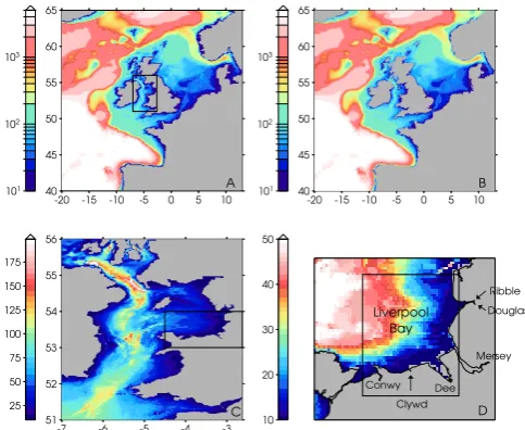
Lan-cashire coasts. The Irish Sea is a typical coastal sea of the northwest European shelf and is subject to large tides, fresh-water influence, high levels of suspended sediment, and hu-man exploitation (e.g. wind farms, oil platforms, shipping). The eastern side of the Sea is shallow, with depths gener-ally less than 50 m. A deeper channel runs down the western side of the Sea with typical depths of 80–100 m, but reaching 150–200 m in parts (Fig. 1c).
Liverpool Bay in particular is considered to be a region of freshwater influence, or ROFI (Simpson, 1997), and is subject to input from several major river systems includ-ing the Conwy, Dee, Mersey, and Ribble estuaries (Fig. 1d). The freshwater input to Liverpool Bay is estimated to be 7.3×10⁹m3 annually (Polton et al., 2011). The interaction of the resulting horizontal salinity gradient and strong tides leads to a cycle of stratified and mixed conditions known as strain induced periodic stratification (SIPS) (Simpson et al., 1990; Howlett et al., 2011; Polton et al., 2011). Briefly, on the ebb tide vertical shear in the tidal current (due to bed fric-tion) means that surface fresh water is advected over saline water, creating stratified conditions. Excluding non-linear ef-fects, on the flood tide the return vertical shear flow restores the stratification to its original profile.
904 C. K. O’Neill et al.: Modelling temperature and salinity in the Irish Sea
51 52 53 54 55 56
-7 -6 -5 -4 -3
25 50 75 100 125 150 175
C 10 20 30 40 50
D Liverpool
Bay
Conwy
Clywd
Mersey
Dee Douglas
Ribble 40
45 50 55 60 65
-20 -15 -10 -5 0 5 10
101
102
103
B 40
45 50 55 60 65
-20 -15 -10 -5 0 5 10
101
102
103
A
Fig. 1. Bathymetry of the model domains in m. Note that plots A and
B use a logarithmic colour scale. In all the models a minimum depth of 10 m is imposed. (A) POLCOMS-AMM. The inset box shows the location of the nested Irish Sea model. (B) NEMO AMM. (C) POLCOMS-IRS, with location of Liverpool Bay indicated by the box. (D) Close up of Liverpool Bay noting the major rivers flowing into the bay. The box marks the area displayed in Fig. 2.
for European Modelling of the Ocean) model is also used. The NEMO code is currently undergoing rapid development and validation by the modelling community.
2 Methods
2.1 Models
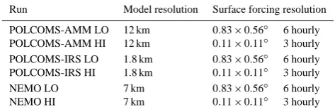
The model domains and formulations used in this study were chosen because they are all standard domains that are widely used, including operationally. Each was run with two dif-ferent atmospheric forcing datasets of difdif-ferent resolutions. This combination of runs allows us to investigate the impact of surface forcing resolution on the models, as well as eval-uating the performance of the newer NEMO configuration against two well established POLCOMS models.
All models were run for the year 2008, with temperature and salinity outputs written hourly so that tidal variability is included in the results. Because of the high temporal resolu-tion of the output, this was restricted to surface and bottom values only. This matches the distribution of the majority of the observations available. A summary of all 6 model runs is given in Table 1.
2.1.1 POLCOMS
POLCOMS is a three-dimensional hydrostatic baroclinic model that was designed to be particularly suited to mod-elling shelf sea regions. A brief summary of notable model
features is given here, but the full description including the equations may be found in Holt and James (2001).
The model grid is formulated on the Arakawa B grid (Arakawa, 1972), in which both velocity components are de-fined on the same points, separated from scalar points by half a grid box. This was chosen because it helps to preserve hor-izontal features such as fronts (Holt and James, 2001). The vertical coordinates used are the s-coordinates of Song and Haidvogel (1994); these are terrain following levels whose spacing is allowed to vary horizontally. Grid points where the water depth is less than a specified critical depth revert to evenly spacedσ-levels (Song and Haidvogel, 1994). The critical depth used here is 150 m, which is deeper than almost all points within the Irish Sea.
The advection scheme used is the piecewise parabolic method (PPM) of Colella and Woodward (1984). The vari-able’s concentration is assumed to vary across a grid box as a parabola, which is then integrated upwind. This method introduces low numerical diffusion giving it good feature-preserving properties (James, 1996, 1997). The turbulence closure scheme used is the κ– scheme (Burchard and Baumert, 1995) implemented by coupling with the General Ocean Turbulence Model (GOTM) (http://www.gotm.net). The POLCOMS implementations used in this study do not apply explicit horizontal diffusion.
Two well-established model domains are used in this study: the Atlantic Margin Model (AMM) (e.g. Wakelin et al., 2009) which covers the northwest shelf area, and a one-way nested Irish Sea Model (IRS) (e.g. Holt and Proctor, 2008). The horizontal resolution of the AMM grid is 1/9◦ lat-itude by 1/6◦longitude, or approximately 12 km. The nested IRS model has resolution 1/60◦ latitude and 1/40◦ longi-tude which is around 1.8 km. The geographic extent and bathymetry of the model domains are shown in Figs. 1a and c. The models have 40 (AMM) and 32 (IRS) internal verti-cal levels, with additional ‘virtual’ levels placed below the sea bed and above the sea surface used in the calculation of flux boundary conditions (Holt and James, 2001). Typi-cal baroclinic Rossby radius values in the western Irish Sea are 1–2 km (Holt and Proctor, 2003), and the semi-diurnal tidal excursion in Liverpool Bay (a more relevant length scale there) is 5–10 km (Hopkins and Polton, 2011). The 1.8 km IRS model is eddy permitting in the western Irish Sea and can resolve the tidal scale, whereas the 12 km AMM model does not resolve either scale.
2.1.2 NEMO
In contrast to POLCOMS, NEMO was originally designed as a global ocean model. Consequently, there are several funda-mental differences between the models. A full description of all model equations and techniques is found in the NEMO manual, which is freely available from the NEMO website (Madec, 2008).
NEMO is implemented on a C grid (Arakawa, 1972) in which u and v velocity components are defined on separate points. NEMO does not currently include the PPM tracer ad-vection scheme used in POLCOMS, though this is planned to be included in a future release. A number of other schemes are available and the TVD (total variance diminishing) op-tion described by Zalesak (1979) is used here. The TVD scheme would be expected to be more diffusive than the PPM scheme (James, 1996). Similarly to POLCOMS, the Canuto et al. (2001)κ–turbulence closure scheme is used. Explicit horizontal diffusion is applied using a Laplacian operator for tracers, and Laplacian and bi-Laplacian operators for mo-mentum.
The vertical coordinate system is similar to the s-coordinate system of Song and Haidvogel (1994) used in POLCOMS, but with a further modification that allows lev-els to run into the sea bed and be lost in areas with very steep slopes. The resulting hybrid z*–s system reduces the slope of the model levels and the associated horizontal pressure gra-dient errors (O’Dea et al., 2012), though this has little impact in Liverpool Bay.
The model domain used in this study is the 1/15◦ lati-tude by 1/9◦longitude (approximately 7 km) Atlantic Mar-gin Model which is based on version 3.2 of the NEMO code (O’Dea et al., 2012). This model is run operationally, cou-pled to the ecosystem model ERSEM, at the UK Met Office providing forecast products to MyOcean users (http://www. myocean.eu). Edwards et al. (2012) find that this operational NEMO-ERSEM model performs better at modelling nutrient and chlorophyll distribution than the POLCOMS-ERSEM system it has replaced. The horizontal extent of the domain is the same as the 12 km POLCOMS-AMM grid, although the NEMO model has 32 internal vertical levels rather than 40. As described above, these become regularly spacedσ-levels at most points within the Irish Sea. The horizontal resolution of 7 km is larger than the Rossby radius in the Irish Sea, but it is only approaching the scale of the tidal excursion within Liverpool Bay.
The model code was further modified for this study to use the same surface flux bulk formulae as POLCOMS, to al-low more direct comparison between the models. River in-put was the same climatological data used in the POLCOMS runs. The lateral boundary forcing was again provided from the Met Office FOAM system. This is the same source as used for the POLCOMS-AMM boundary forcing, though files were provided separately as the models require
differ-Table 1. Summary of the model runs compared in this study
Run Model resolution Surface forcing resolution POLCOMS-AMM LO 12 km 0.83×0.56◦ 6 hourly POLCOMS-AMM HI 12 km 0.11×0.11◦ 3 hourly POLCOMS-IRS LO 1.8 km 0.83×0.56◦ 6 hourly POLCOMS-IRS HI 1.8 km 0.11×0.11◦ 3 hourly NEMO LO 7 km 0.83×0.56◦ 6 hourly NEMO HI 7 km 0.11×0.11◦ 3 hourly
ent input formats. The runs were initialised from a restart file created at the end of a spin-up run.
2.1.3 Surface forcing
Surface heat fluxes were calculated internally in all three models using bulk formulae following the COARE v3 algo-rithm (Fairall et al., 2003). The input parameters required are air temperature, air pressure, wind speed, specific humidity, cloud cover, and precipitation. The input atmospheric data were provided by Met Office numerical weather prediction models.
The impact of changing surface forcing resolution was in-vestigated by running two simulations with each model that are identical in every respect other than the surface forcing data. Two Met Office datasets were used: a global atmo-spheric model, which has resolution of 6 h and 0.83×0.56◦, and a northeast Atlantic model with resolution of 3 h and 0.11×0.11◦. The two forcing datasets have been checked for consistency and are well correlated with each other. The higher resolution dataset does not cover a wide enough geo-graphic area to be used to force the POLCOMS-AMM and NEMO-AMM models, so the outer areas were filled by in-terpolating the lower resolution global dataset in time and space. For the rest of this paper, the low and high resolution forcing datasets are labelled LO and HI, respectively. The three models all interpolate the forcing data to their model grid resolution at run time.
2.2 Observations
The observational data we use to evaluate model perfor-mance were collected as part of the Liverpool Bay Coastal Observatory (CObs) and are freely available (Howarth and Palmer, 2011). Three sources of observational data are used in this study:
– Regularly sampled CTD (conductivity, temperature, depth) survey grid in Liverpool Bay.
– Instrumented ferry that runs across the Irish Sea from Liverpool to Dublin or Belfast.
– Mooring located at Site A in Liverpool Bay.
906 C. K. O’Neill et al.: Modelling temperature and salinity in the Irish Sea
Table 2. List of Liverpool Bay Coastal Observatory CTD survey
cruise dates in 2008
January 10–11 March 11–15 April 16–17 May 13–16 June 25–26
July 30–August 01 September 10–12
October 21–23 December 10–12
mooring and CTD grid are located) as well as in the offshore Irish Sea (the instrumented ferry), and provides confidence that the results are robust, as they are independent from one another. We have not used the available satellite-measured sea surface temperature data as these are already assimilated into the atmospheric model that is used to force the models.
2.2.1 CTD survey
CTD profiles were taken on regular cruises about every 6 weeks through the year, with measurements taken at 0.5 dBar intervals. Cruise dates in 2008 are shown in Table 2. There are a total of 34 stations spaced approximately on a 5-nautical-mile grid (Howarth and Palmer, 2011), though they were not all sampled on every cruise. There were 9 cruises within the study year during which a total of 246 CTD pro-files were taken; this included one 25-h station at site A where measurements were taken half-hourly. Figure 2 shows the mean location of the stations and the total number of pro-files taken at each one during 2008.
2.2.2 Ferry
As a joint initiative between CObs and the FerryBox project, a commercial ferry run by Nofolkline (later DFDS Seaways) was fitted with sensors measuring near-surface parameters including temperature, conductivity, turbidity and chloro-phyll (Howarth and Palmer, 2011; Balfour et al., 2007). Mea-surements were taken every 10 s, and sent remotely to data servers approximately every 15 min. The ferry ran daily from Liverpool to Dublin (or occasionally Belfast), effectively giv-ing a repeated transect across the centre of the Irish Sea. The temporal coverage in 2008 is 2 January–22 October. Because the 10 s sample interval is far beyond the temporal resolu-tion of the model outputs, the dataset was sub-sampled ap-proximately every 10 min. In addition, any points where the recorded salinity was less than 20 were assumed to be within the dock and were not used. Points further north than 53.8◦N were also excluded to keep the focus on the east–west tran-sect. This gives a total of 15102 data points which were used in this study.
−4˚00'
−3˚30'
−3˚00'
53˚10'
53˚20'
53˚30'
53˚40'
53˚50'
−4˚00'
−3˚30'
−3˚00'
53˚10'
53˚20'
53˚30'
53˚40'
53˚50'
3
3
3
4
5
5
3
3
3
4
7
5
4
4
5
7
15
6
3
3
6
5
7
5
4
5
7
72
8
6
5
6
7
8
Fig. 2. Mean location of CTD survey stations and number of profiles
collected in 2008. Site A (location of the mooring) is indicated by the dashed square.
2.2.3 Site A mooring
A Centre for Environment, Fisheries and Aquaculture Sci-ence (CEFAS) “SmartBuoy” mooring measuring near sur-face temperature and conductivity, as well as various bio-geochemical parameters, is located at 53◦31.80N, 3◦21.60W (referred to as Site A, and indicated by the dashed square in Fig. 2). Observations are recorded approximately hourly and after accounting for data gaps there are 7599 tempera-ture and 6591 salinity observations in 2008. Co-located with the mooring is a bed frame also measuring temperature and salinity. The number of observations where both surface and bottom data are present is 7027 for temperature and 4042 for salinity.
The location of site A presents distinct challenges for model validation since it is within a region of strong lateral salinity gradients that are advected with the ebb and flood tide leading to significant intratidal variability. Therefore, these data are preprocessed by filtering in one of two ways before making model comparisons:
1. Time series analyses are graphically presented (Figs. 6, 7, 10) by computing a running mean with a moving win-dow of 175 h (7×25) to give a simple tidal filter. 2. Before making statistical comparison with the model
re-sults, the tidal signal was removed using a Doodson X0
after the reference value. The residual data were then also smoothed using a 6-h running average to remove any remaining high frequency noise.
For consistent intercomparisons at this site, the same pro-cessing was applied to the model results after being spatially interpolated to the site A location.
2.3 Analysis
For each observation type, the model results were interpo-lated in space–time to the locations of the observations. Re-sults were then compared on a point by point basis. This is a strict test of the models, as there is no account taken of a slight difference in phase or location of features such as the Mersey river plume. Note that the CTD and ferry obser-vations, and the model results compared against them, were not adjusted to remove the tide.
In order to objectively and systematically compare the per-formance of different models, it is necessary to make use of quantitative skill score metrics. In this paper we use the squared correlation coefficientr2, and a cost functionχ fol-lowing that used by Holt et al. (2005). RMS error is also cal-culated to give an idea of the size of model errors in physical terms:E=
qPN
(Mn−On)2
N , where N is the number of data
points, andOn andMn are observed and modelled values,
respectively.
The correlation coefficientr is defined by Eq. (1), and is a measure of how well the modelled and observed data fit a linear least squares relationship. A perfect fit has a value of
r=1, whereas non-varying model data would have a value ofr=0. The squared value,r2, represents the proportion of observed variability that is reproduced by the model. In this case we use the formr|r|, so that the distinction between positive and negative correlation is retained.
r=
PN
n=1 On− ¯O
Mn− ¯M q
PN
n=1 On− ¯O
2PN
n=1 Mn− ¯M 2
(1)
¯
OandM¯ are the mean of the observed and modelled values. The cost function used in this study is defined by Eq. (2) (Holt et al., 2005).
χ2= 1
N σ2 o
N X
n=1
(Mn−On)2, (2)
whereσo2is the variance of the observations. This type of cost function is recommended by Allen et al. (2007, p. 402) due to its non-linearity, which rewards a good fit and punishes poor fit.
A cost function is a measure of the ratio of model error to the observed variance, and this particular form may be thought of as the RMS error normalised by observed standard deviation. We would expect a model with predictive skill to
produce values ofχ <1 (Holt et al., 2005), i.e. the RMS er-ror is smaller than the standard deviation of the observations. Holt et al. (2005) additionally identify the thresholdχ=0.4 as representing a “well modelled” variable.
3 Results
3.1 Surface temperature
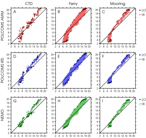
Figure 3 gives an overview of the results, with the model re-sults plotted against observations for every comparison point. The plots show that all three models show a clear linear rela-tionship between modelled and observed temperature. Closer inspection of the plots shows that all the models tend to over-estimate warm summer temperatures, and underover-estimate cold winter values. This bias was reduced when the HI surface forcing was used.
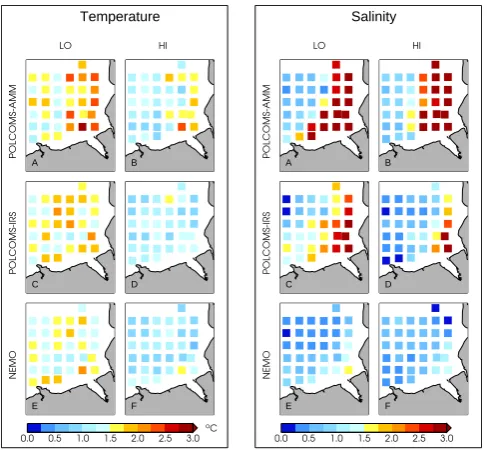
The ferry and CTD comparisons also provide information on the spatial variation in model errors, shown in Figs. 4 (ferry) and 5 (CTD). RMS errors compared to the ferry data show a significant east–west difference in all runs using LO forcing, with higher errors in the eastern half of the Irish Sea (Fig. 4). This spatial pattern remains in the lowest res-olution POLCOMS-AMM model with HI forcing, whereas the POLCOMS-IRS and NEMO errors are more homoge-neous (and lower) across the observed region. RMS errors for each CTD station (Fig. 5) show a less clear spatial sig-nal than could be seen in the ferry comparison, though the POLCOMS-AMM model appears to be generally worse in the east of Liverpool Bay, along the coast. Though it must be remembered that at 12 km resolution only a limited per-formance can be expected on these spatial scales. All three models show a clear improvement when using the HI forcing (Fig. 5 right-hand panels).
The r2 correlation values (Tab. 3) show that all models perform well at capturing the large-scale seasonal temper-ature cycle with r2values greater than 0.9. The values are similar across the models, although the 12 km POLCOMS-AMM model’s correlation is consistently slightly lower than the other models. There is very little difference between the LO and HI results.
908 C. K. O’Neill et al.: Modelling temperature and salinity in the Irish Sea
Discussion
P
ap
er
|
Discussion
P
ap
er
|
Discussion
P
ap
er
|
Di
scuss
ion
P
ap
er
|
Fig. 3.Scatter plots of modelled surface temperature (Y axis) against observed surface temperature (X axis). These plots include all observations from 2008. Panels ABC: POLCOMS-AMM, panels DEF: POLCOMS-IRS, panels GHI: NEMO.
22
Fig. 3. Scatter plots of modelled surface temperature (y-axis)
against observed surface temperature (x-axis). These plots include all observations from 2008. Panels A, B, C: POLCOMS-AMM; panels D, E, F: POLCOMS-IRS; panels G, H, I: NEMO.
The 7×25-h running mean temperature and the difference from this running mean for the mooring data and the models are shown in Fig. 6. The running mean surface temperature (panel a) is dominated by the very strong annual cycle and shows that all three models are too cold in winter and too warm in summer. This is improved when using the HI forc-ing dataset. The POLCOMS-IRS and NEMO results are very similar to each other, as is POLCOMS-AMM in the second half of the year. The deviation from the running mean (panel b) indicates that NEMO appears to be better reproducing the high frequency tidal advection of surface temperature.
3.2 Surface salinity
Figure 8 shows scatter plots for all surface model– observation pairs over the study year. It is clear that none of the models predicts surface salinity as well as they do temper-ature. This is particularly striking when comparing the mod-els with the mooring data. Both POLCOMS modmod-els overes-timate the salinity range, whereas NEMO generally matches or underestimates the observed range. Both POLCOMS runs display a clear spatial variation in RMS error with high errors in the region of the Mersey plume, seen in both the CTD and ferry comparisons (Figs. 5 and 9). NEMO shows a similar, but much weaker, pattern. NEMO also shows lower errors than either of the POLCOMS runs in Liverpool Bay and the eastern Irish Sea, but is slightly worse than POLCOMS in the western Irish Sea.
The r2 correlation values (Table 3) range from 0.3–0.6 against the CTD and 0.6–0.8 against the ferry observations.
F D B
HI LO
A
POLCOMS-AMM
C
POLCOMS-IRS
E
NEMO
0.0 0.5 1.0 1.5 2.0 2.5
oC
Fig. 4. Model RMS error in surface temperature compared with
ferry observations. Due to the large number of observations, the results have been spatially averaged within 30by 1.20bins to pro-duce this plot. (A) POLCOMS-AMM LO; (B) POLCOMS-AMM HI; (C) POLCOMS-IRS LO; (D) POLCOMS-IRS HI; (E) NEMO LO; and (F) NEMO HI.
This suggests the models do have some predictive skill, par-ticularly in the open sea areas where most of the ferry mea-surements are taken, although they do not capture the sea-sonal variability as well as they do with temperature. The comparison with the mooring at site A on the other hand is very poor in all models withr|r|between−0.1 and 0.0. This suggests that none of the models are correctly predicting the salinity variability within Liverpool Bay. This is confirmed by Fig. 10, which shows that on longer timescales, the mod-els’ variabilities do not match the observed patterns at site A.
The cost function values (Table 4) also show that the model performance is significantly poorer (higherχ) than was the case with temperature. However, the NEMO mod-els do produce values less than 1 against the CTD and ferry observations. The POLCOMS-AMM cost function is poor against all the observations, with values from 1.6–7.8. This is reflected in high overall RMS errors (Table 6). There is a less homogeneous response to the change in surface forcing than was seen in the temperature comparison, with improvements in some model–observation comparisons (e.g. IRS vs. CTD) and little change in others (e.g. POLCOMS-AMM vs. CTD). There is a more consistent improvement in the overall statistics when the models are compared with the ferry data, which covers more open sea regions away from the Liverpool Bay ROFI.
F D B Temperature
HI LO
A
POLCOMS-AMM
C
POLCOMS-IRS
E
NEMO
0.0 0.5 1.0 1.5 2.0 2.5 3.0
oC
F D B Salinity
HI LO
A
POLCOMS-AMM
C
POLCOMS-IRS
E
NEMO
0.0 0.5 1.0 1.5 2.0 2.5 3.0
Fig. 5. Model RMS error compared with CTD observations for
surface temperature (left) and surface salinity (right). Results have been averaged within the survey stations to produce this plot. (A) POLCOMS-AMM LO; (B) POLCOMS-AMM HI; (C) POLCOMS-IRS LO; (D) POLCOMS-IRS HI; (E) NEMO LO; and
(F) NEMO HI.
results from the same POLCOMS Irish Sea model for the year 2010, where the model qualitatively appears to perform better than we find in this study.
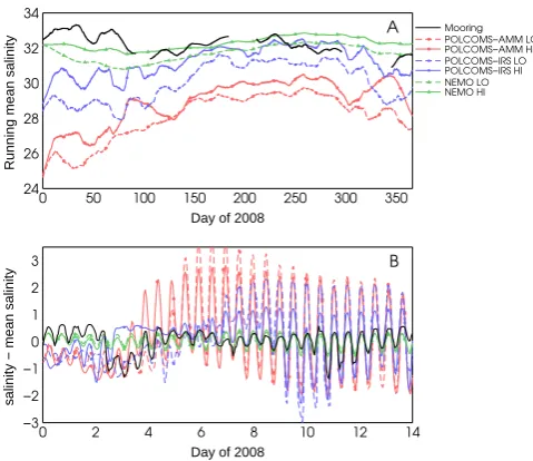
Figure 10b shows the difference from the mean salinity for the mooring data and models at site A. It is clear that both POLCOMS models are significantly overestimating the salinity tidal variability. On the longer timescales indicated by the running mean salinity (Fig. 10a), there is also a large variation between the models. Again NEMO shows less vari-ability than either of the POLCOMS models, consistent with the RMS errors shown in Table 6. Both POLCOMS models are generally too fresh, especially POLCOMS-AMM which is well below the observed salinity at site A, though this is improved when the HI surface forcing is used.
4 Discussion
The overall results show that all the models used in this study display significantly higher skill at predicting surface tem-perature than they do for salinity, particularly in the near coastal region of Liverpool Bay where the principal driving influence is the poorly determined freshwater forcing (Polton et al., 2011). By comparing the different model runs, we can assess the relative importance of surface forcing resolution and model type on the predictive skill.
Table 3.r|r|correlation of model surface temperature and salinity
compared with observations. Columns labelled C are against CTD observations, F against ferry observations, and M against mooring observations.
Model Temperature Salinity
C F M C F M
POLCOMS-AMM LO 0.92 0.95 0.97 0.40 0.66 −0.16
POLCOMS-AMM HI 0.94 0.96 0.97 0.36 0.71 −0.15
POLCOMS-IRS LO 0.96 0.97 0.98 0.55 0.68 −0.03
POLCOMS-IRS HI 0.97 0.98 0.98 0.61 0.74 −0.03
NEMO LO 0.96 0.97 0.99 0.48 0.69 −0.01
NEMO HI 0.97 0.98 0.98 0.52 0.78 −0.00
Table 4. Cost functionχof model surface temperature and salinity
compared with observations. Columns labelled C are against CTD observations, F against ferry observations, and M against mooring observations.
Model Temperature Salinity
C F M C F M
POLCOMS-AMM LO 0.54 0.55 0.67 3.54 1.95 7.75
POLCOMS-AMM HI 0.45 0.42 0.45 3.57 1.61 6.52
POLCOMS-IRS LO 0.48 0.45 0.48 2.27 1.27 4.49
POLCOMS-IRS HI 0.37 0.32 0.35 1.43 0.78 2.77
NEMO LO 0.43 0.45 0.48 0.84 0.73 1.70
NEMO HI 0.33 0.32 0.35 0.74 0.60 1.19
4.1 Impact of surface forcing resolution
The surface temperature cost function against all three obser-vation sources was significantly improved when the higher resolution forcing data were used, from 0.43–0.47 to 0.32– 0.33. This corresponds to a general improvement in the in-stantaneous temperatures throughout the record. There was, however, little increase in ther2values since this is a mea-sure of the skill in reproducing the annual cycle, which was already very high with values greater than 0.95 in both runs. This is because ther2score is dominated by the large sea-sonal cycle in temperature that the models capture well over-all. Although the value ofr2does not change much, Fig. 6a shows that the summer high and winter low biases are re-duced in all the models when the HI forcing is used.
910 C. K. O’Neill et al.: Modelling temperature and salinity in the Irish Sea
Table 5. Mean RMS error of model surface temperature compared
with CTD, ferry, and mooring observations. The mean values are calculated by averaging in time over the entire year, as well as hori-zontally for the CTD and ferry comparisons. The percentage change in RMS error after increasing the surface forcing resolution is also indicated.
Model CTD Ferry Mooring
POLCOMS-AMM LO 1.75 1.65 2.60
POLCOMS-AMM HI 1.45 −17 % 1.27 −23 % 1.75 −33 %
POLCOMS-IRS LO 1.58 1.35 1.86
POLCOMS-IRS HI 1.20 −24 % 0.95 −30 % 1.34 −28 %
NEMO LO 1.40 1.35 1.86
NEMO HI 1.07 −24 % 0.96 −29 % 1.36 −27 %
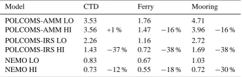
Table 6. Mean RMS error of model surface salinity compared with
CTD, ferry, and mooring observations. The mean values are calcu-lated by averaging in time over the entire year, as well as horizon-tally for the CTD and ferry comparisons. The percentage change in RMS error after increasing the surface forcing resolution is also indicated.
Model CTD Ferry Mooring
POLCOMS-AMM LO 3.53 1.76 4.71
POLCOMS-AMM HI 3.56 +1 % 1.47 −16 % 3.96 −16 %
POLCOMS-IRS LO 2.26 1.16 2.72
POLCOMS-IRS HI 1.43 −37 % 0.72 −38 % 1.69 −38 %
NEMO LO 0.83 0.67 1.03
NEMO HI 0.73 −12 % 0.55 −18 % 0.72 −30 %
the Irish Sea. The overall temperature RMS error (Table 5) was reduced by around 20–30 % when using the HI forcing.
The running mean temperature (Fig. 6a) clearly shows that the surface forcing resolution has more impact on the seasonal cycle results than the choice of model, particularly the choice between POLCOMS-IRS and NEMO. An unpub-lished preliminary NEMO run which was forced by hourly surface flux data (rather than bulk parameters) produced bet-ter results again than either of the runs discussed here, partic-ularly in the winter. The high frequency variability (Fig. 6b) on the other hand is generally similar in the LO and HI runs, especially in NEMO.
Surface salinity showed a somewhat weaker response to the change in forcing, with RMS errors reduced in some ar-eas, particularly against the ferry data, but increased in oth-ers (Figs. 5 and 9). This is not entirely surprising since we would expect surface temperature to be more sensitive to changes in the surface forcing, as it is directly forced by at-mospheric heat fluxes. Salinity in the Liverpool Bay region on the other hand is predominantly influenced by the balance between riverine and oceanic freshwater inputs and is less strongly linked to surface fluxes. However, an unpublished preliminary NEMO run which used hourly surface flux forc-ing further improved results for salinity as well as temper-ature. Further work is needed to establish whether this was
−2.0 −1.5 −1.0 −0.5 0.0 0.5 1.0 1.5 2.0
temperature − mean temperature oC 0 2 4 6 8 10 12 14
Day of 2008
B 4
6 8 10 12 14 16 18 20
Running mean temperature oC
0 50 100 150 200 250 300 350
Day of 2008
A Mooring
POLCOMS−AMM LO POLCOMS−AMM HI POLCOMS−IRS LO POLCOMS−IRS HI NEMO LO NEMO HI
Fig. 6. (A) 175-h running average surface temperature at site A. (B)
Deviation of surface temperature from the running average. Note that only the first 14 days are plotted on panel B, for clarity.
due to the improved resolution, or more accurate flux values than are obtained from the bulk formulae.
4.2 Differences between models
It is clear from the spatial maps of model error and the ob-jective metrics that the 12 km POLCOMS-AMM model does not perform as well in Liverpool Bay as either of the other models used, particularly with surface salinity. This is not un-expected given the low resolution of the model, and it would perhaps be unfair to expect it to perform any better in this region. However, it is important to note that in the western Irish Sea the model results are comparable with the higher resolution models. Overall, POLCOMS-AMM was shown to have skill in modelling both the annual cycle of surface tem-perature, withr2>0.9, and the tidal variability with the cost functionχ <1.
The salinity error map associated with the POLCOMS-AMM model on the other hand stands out as different to all the other models, with a very clearly defined area of large er-ror in Liverpool Bay seen in both the ferry (Fig. 9) and CTD (Fig. 5) comparisons. The front associated with the freshwa-ter plume from the River Mersey is known to move by up to 0.5◦east–west over the spring–neap cycle (Polton et al., 2011; Hopkins and Polton, 2011). This is equivalent to fewer than 3 grid boxes within the POLCOMS-AMM model, so we could expect to have large errors in the position of the front with this model.
−3.0 −2.5 −2.0 −1.5 −1.0 −0.5 0.0
Surface−bottom salinity
0 25 50 75 100 125
Day of 2008
B
−2.5 −2.0 −1.5 −1.0 −0.5 0.0 0.5 1.0 1.5 2.0 2.5
Surface−bottom temperature
oC
0 50 100 150 200 250 300 350
Day of 2008
A Mooring
POLCOMS−AMM HI
POLCOMS−IRS HI
NEMO HI
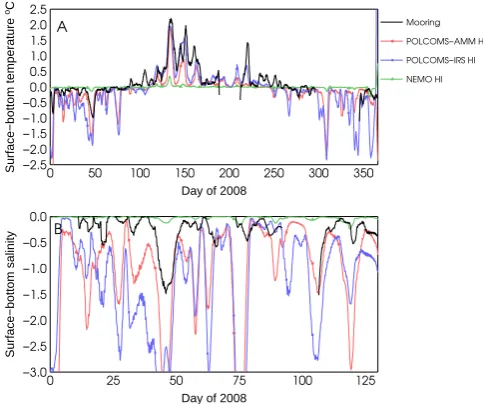
Fig. 7. 175-h running average surface–bottom temperature (A) and
salinity (B) difference from the mooring data and HI model runs at site A. Note that only the first 130 days are plotted for salinity, for clarity.
Discussion
P
ap
er
|
Discussion
P
ap
er
|
Discussion
P
ap
er
|
Di
scuss
ion
P
ap
er
|
Fig. 8. Scatter plots of modelled surface salinity (Y axis) against observed surface salinity (X axis). These plots include all observations from 2008. Panels ABC: POLCOMS-AMM, panels DEF: POLCOMS-IRS, panels GHI: NEMO.
27
Fig. 8. Scatter plots of modelled surface salinity (y-axis) against
observed surface salinity (x-axis). These plots include all obser-vations from 2008. Panels ABC: POLCOMS-AMM; panels DEF: POLCOMS-IRS; panels GHI: NEMO.
comparable, this is not to say that the sources of errors in the two models are the same.
There are large differences in salinity between the mod-els on both the tidal and longer timescales (Fig. 10) at site A. Both POLCOMS models systematically overestimate the high frequency tidal variability in salinity at site A (Fig. 10b),
F D B
HI LO
A
POLCOMS-AMM
C
POLCOMS-IRS
E
NEMO
0.0 0.5 1.0 1.5 2.0 2.5 3.0
Fig. 9. RMS error in model surface salinity compared with ferry
observations. Due to the large number of observations, the results have been spatially averaged within 30by 1.20bins to produce this plot. (A) POLCOMS-AMM LO; (B) POLCOMS-AMM HI; (C) POLCOMS-IRS LO; (D) POLCOMS-IRS HI; (E) NEMO LO; and
(F) NEMO HI.
whereas the variability of NEMO is much more similar to the observations. With all three models using the same river in-put data, this is a direct consequence of the models’ abilities to simulate the strength of the front in Liverpool Bay. Fig-ure 11 shows the variation with longitude of the horizontal salinity gradient of the models and the ferry and CTD ob-servations. All three models reproduce the lower gradients in the bulk of the Irish Sea, but both POLCOMS models sig-nificantly overestimate the strength of the salinity gradient east of 4◦W, in Liverpool Bay. The NEMO model more ac-curately reproduces the observed gradient in this area. As all the models in this study were forced by the same climatolog-ical river input data, the likely source for this difference is the more diffusive horizontal mixing scheme used in NEMO.
Surface–bottom differences in temperature and salinity at site A are shown in Fig. 7. These are 25-h running mean values to show the persistent stratification rather than inter-mittent SIPS conditions. Both POLCOMS models are fre-quently persistently stratified, and generally more strongly than is shown by the observations, particularly with salinity. However, the POLCOMS models do capture the broad an-nual cycle in the temperature difference with warmer water over cold in the summer and vice versa in winter. NEMO in contrast is consistently well mixed and shows little variation over the year.
5 Conclusions
912 C. K. O’Neill et al.: Modelling temperature and salinity in the Irish Sea
−3 −2 −1 0 1 2 3
salinity − mean salinity
0 2 4 6 8 10 12 14
Day of 2008
B
24 26 28 30 32 34
Running mean salinity
0 50 100 150 200 250 300 350 Day of 2008
A Mooring POLCOMS−AMM LO POLCOMS−AMM HI POLCOMS−IRS LO POLCOMS−IRS HI NEMO LO NEMO HI
Fig. 10. (A) 175-h running average surface salinity at site A. (B)
Deviation of surface salinity from the running average. Note that only the first 14 days are plotted on panel (B), for clarity.
metrics. It is clear that much work still needs to be done to improve our ability to accurately model salinity in this complex regime. Liverpool Bay is highly influenced by the large freshwater input from several major river basins, so the model performance may have been limited in this area by the use of climatological river flow forcing data.
The resolution of surface forcing input to the models is found to be important, and increased forcing resolution uni-versally increased the models’ skills in forecasting surface temperature. In particular, the 7 km NEMO model performed as well as the 1.8 km POLCOMS model when both used the same forcing dataset. This indicates the importance of match-ing surface forcmatch-ing resolution with the ocean model resolu-tion – increasing ocean model resoluresolu-tion is costly whereas improving the forcing data resolution could potentially bring as much benefit. This is particularly relevant for decadal modelling where it is not practical to use high resolution ocean models. Salinity in Liverpool Bay is less clearly linked to the surface fluxes and surface salinity errors were not al-ways improved in the runs with high resolution forcing data. Improvements in river input forcing and the background dy-namics such as stratification have more impact on the mod-els’ skills in predicting salinity.
The POLCOMS and NEMO models differ in their ability to represent the density front in Liverpool Bay. POLCOMS is specifically designed to preserve frontal quantities with its piecewise parabolic advection scheme. NEMO on the other hand is more diffusive. At fine resolution, in Liverpool Bay, it appears here that the non-diffusive advection scheme is not diffusive enough. While this is appropriate for coarser reso-lution models like the 12 km POLCOMS-AMM, or in deeper water frontal environments such as the western Irish Sea, the
0 5 10 15
Salinity gradient magnitude PSU/degree
−6.0 −5.5 −5.0 −4.5 −4.0 −3.5 −3.0
Longitude Site A
Ferry CTD
POLCOMS AMM HI POLCOMS IRS HI NEMO HI
Fig. 11. Magnitude of horizontal salinity gradient for models and
observations along the latitude of site A mooring (53.53◦N). Only HI forcing results are shown, for clarity.
more diffusive advection scheme used in NEMO better cap-tures the Liverpool Bay tidal variability.
Overall, the performance of the NEMO-AMM model is very promising, with objective skill scores as good as or bet-ter than the higher resolution POLCOMS-IRS model. In par-ticular, NEMO reproduces the horizontal salinity gradient in Liverpool Bay more accurately than POLCOMS. How-ever, we should note that NEMO underestimates the strati-fication within Liverpool Bay (whereas POLCOMS is over-stratified), and the reasons behind this need to be further in-vestigated. We look forward to the continuing development and improvement of NEMO which may yield better future results when modelling salinity in Liverpool Bay.
Acknowledgements. This work has been funded by the MyOcean
programme as part of Work Package 7. The authors also wish to thank all those involved in the collection of the observational data, which were provided by the Liverpool Bay Coastal Observatory. The manuscript has benefitted from the constructive comments of three anonymous reviewers.
Edited by: J. A. Johannessen
References
Allen, J. I., Holt, J. T., Blackford, J., and Proctor, R.: Error quan-tification of a high-resolution coupled hydrodynamic-ecosystem coastal-ocean model: Part 2. Chlorophyll-a, nutrients and SPM, J. Mar. Syst., 68, 381–404, doi:10.1016/j.jmarsys.2007.01.005, 2007.
Arakawa, A.: Design of the UCLA general circulation model, Tech. Rep. 7, Dept. of Meteorology, University of California, 1972. Balfour, C. A., Howarth, M. J., Smithson, M. J., Jones, D. S., and
Pugh, J.: The use of ships of opportunity for Irish Sea based oceanographic measurements, in: Oceans ’07 IEEE Aberdeen, Conference Proceedings. Marine challenges: coastline to deep sea., IEEE Catalog No. 07EX1527C, 2007.
ocean forecasting, J. Mar. Syst., 25, 1–25, doi:10.1016/S0924-7963(00)00005-1, 2000.
Burchard, H. and Baumert, H.: On the performance of a mixed-layer model based on the κ- turbulence closure, J. Geophys. Res., 100, 8523–8540, doi:10.1029/94JC03229, 1995.
Canuto, V. M., Howard, A., Cheng, Y., and Dubovikov, M. S.: Ocean Turbulence. Part I: One-Point Closure Model – Momen-tum and Heat Vertical Diffusivities, J. Phys. Oceanogr., 31, 1413–1426, 2001.
Colella, P. and Woodward, P. R.: The Piecewise Parabolic Method (PPM) for gas-dynamical situations, J. Comput. Phys., 54, 174– 201, doi:10.1016/0021-9991(84)90143-8, 1984.
Edwards, K. P., Barciela, R., and Butensch¨on, M.: Validation of the NEMO-ERSEM operational ecosystem model for the North West European Continental Shelf, Ocean Sci. Discuss., 9, 745– 786, doi:10.5194/osd-9-745-2012, 2012.
Fairall, C. W., Bradley, E. F., Hare, J. E., Grachev, A. A., and Ed-son, J. B.: Bulk parameterization of air-sea fluxes: Updates and verification for the COARE algorithm, J. Climate, 16, 571–591, doi:10.1175/1520-0442(2003)016<0571:BPOASF>2.0.CO;2, 2003.
Holt, J. T. and James, I. D.: An s coordinate density evolving model of the northwest European continental shelf: 1, Model descrip-tion and density structure, J. Geophys. Res., 106, 14015–14034, doi:10.1029/2000JC000304, 2001.
Holt, J. and Proctor, R.: The Role of Advection in De-termining the Temperature Structure of the Irish Sea, J. Phys. Oceanogr., 33, 2288–2306, doi:10.1175/1520-0485(2003)033<2288:TROAID>2.0.CO;2, 2003.
Holt, J. and Proctor, R.: The seasonal circulation and vol-ume transport on the northwest European continental shelf: A fine-resolution model study, J. Geophys. Res., 113, C06021, doi:10.1029/2006JC004034, 2008.
Holt, J. T., Allen, J. I., Proctor, R., and Gilbert, F.: Er-ror quantification of a high-resolution coupled hydrodynamic-ecosystem coastal-ocean model: Part 1 model overview and as-sessment of the hydrodynamics, J. Mar. Syst., 57, 167–188, doi:10.1016/j.jmarsys.2005.04.008, 2005.
Hopkins, J. and Polton, J. A.: Scales and structure of frontal ad-justment and freshwater export in a region of fresh water influ-ence, Ocean Dynam., 62, 45–62, doi:10.1007/s10236-011-0475-7, 2011.
Howarth, J. and Palmer, M.: The Liverpool Bay Coastal Observa-tory, Ocean Dynam., 61, 1917–1926, doi:10.1007/s10236-011-0458-8, 2011.
Howlett, E. R., Rippeth, T. P., and Howarth, J.: Processes con-tributing to the evolution and destruction of stratification in the Liverpool Bay ROFI, Ocean Dynam., 61, 1403–1419, doi:10.1007/s10236-011-0402-y, 2011.
James, I. D.: Advection schemes for shelf sea models, J. Mar. Syst., 8, 237–254, doi:10.1016/0924-7963(96)00008-5, 1996. James, I. D.: A numerical model of the development of anticyclonic
circulation in a gulf-type region of freshwater influence, Cont. Shelf. Res., 17, 1803–1816, doi:10.1016/S0278-4343(97)00052-6, 1997.
Madec, G.: NEMO ocean engine, Tech. Rep. 27, Note du Pole de mod´elisation, Institut Pierre-Simon Laplace (IPSL), available at: http://www.nemo-ocean.eu/About-NEMO/Reference-manuals, ISSN 1288–1619, 2008.
O’Dea, E., Arnold, A., Edwards, K., Furner, R., Hyder, P., Mar-tin, M., Siddorn, J., Storkey, D., While, J., Holt, J., and Liu, H.: An operational ocean forecast system incorporating NEMO and SST data assimilation for the tidally driven European North-West shelf, J. Operat. Oceanogr., 5, 3–17, 2012.
Polton, J. A., Palmer, M. R., and Howarth, M. J.: Physical and dynamical oceanography of Liverpool Bay, Ocean Dynam., 61, 1421–1439, doi:10.1007/s10236-011-0431-6, 2011.
Pugh, D.: Tides, Surges and Mean Sea Level, John Wiley and Sons, 1987.
Simpson, J. H.: Physical processes in the ROFI regime, J. Mar. Syst., 12, 3–15, doi:10.1016/S0924-7963(96)00085-1, 1997. Simpson, J. H., Brown, J., Matthews, J., and Allen, G.: Tidal
Strain-ing, Density Currents, and Stirring in the Control of Estuar-ine Stratification, Estuaries, 13, 125–132, doi:10.2307/1351581, 1990.
Song, Y. and Haidvogel, D.: A semi-implicit ocean circu-lation model using a generalized topography-following coordinate system, J. Comput. Phys., 115, 228–244, doi:10.1006/jcph.1994.1189, 1994.
Wakelin, S. L., Holt, J. T., and Proctor, R.: The influence of initial conditions and open boundary conditions on shelf circulation in a 3-D ocean-shelf model of the North East Atlantic, Ocean Dy-nam., 59, 67–81, doi:10.1007/s10236-008-0164-3, 2009. Young, E. F. and Holt, J. T.: Prediction and analysis of long-term
variability of temperature and salinity in the Irish Sea, J. Geo-phys. Res., 112, C01008, doi:10.1029/2005JC003386, 2007. Zalesak, S. T.: Fully Multidimensional Flux-Corrected Transport