Intercomparison of snow depth retrievals over Arctic sea ice from radar data acquired by Operation IceBridge

(1)

https://doi.org/10.5194/tc-11-2571-2017

Intercomparison of snow depth retrievals over Arctic sea ice from

radar data acquired by Operation IceBridge

Ron Kwok1, Nathan T. Kurtz2, Ludovic Brucker2,3, Alvaro Ivanoff4, Thomas Newman5, Sinead L. Farrell6,7, Joshua King8, Stephen Howell8, Melinda A. Webster2, John Paden9, Carl Leuschen9, Joseph A. MacGregor2, Jacqueline Richter-Menge10, Jeremy Harbeck4, and Mark Tschudi11

1_{Jet Propulsion Laboratory, California Institute of Technology, Pasadena, California, USA}

2_{Cryospheric Sciences Laboratory, NASA Goddard Space Flight Center, Greenbelt, Maryland, USA}

3_{Universities Space Research Association, Goddard Earth Sciences Technology and Research Studies and Investigations,}

Columbia, MD, USA

4_{ADNET Systems Inc., Lanham, MD, USA}

5_{Department of Atmospheric Physics, University of Toronto, Toronto, Ontario, Canada}

6_{Earth System Science Interdisciplinary Center, University of Maryland, College Park, Maryland, USA}

7_{Laboratory for Satellite Altimetry, Satellite Oceanography and Climatology Division, NOAA Center for Weather and}

Climate Prediction, College Park, Maryland, USA

8_{Climate Research Division, Environment and Climate Change Canada, Toronto, Ontario, Canada} 9_{Center for Remote Sensing of Ice Sheets, The University of Kansas, Lawrence, Kansas, USA} 10_{Institute of Northern Engineering, University of Alaska Fairbanks, Fairbanks, Alaska, USA}

11_{Colorado Center for Astrodynamics Research, University of Colorado Boulder, Boulder, Colorado, USA}

Correspondence to:Ron Kwok ([email protected])

Received: 1 June 2017 – Discussion started: 15 June 2017

Revised: 3 October 2017 – Accepted: 7 October 2017 – Published: 13 November 2017

Abstract.Since 2009, the ultra-wideband snow radar on Op-eration IceBridge (OIB; a NASA airborne mission to sur-vey the polar ice covers) has acquired data in annual cam-paigns conducted during the Arctic and Antarctic springs. Progressive improvements in radar hardware and data pro-cessing methodologies have led to improved data quality for subsequent retrieval of snow depth. Existing retrieval algo-rithms differ in the way the air–snow (a–s) and snow–ice (s–i) interfaces are detected and localized in the radar re-turns and in how the system limitations are addressed (e.g., noise, resolution). In 2014, the Snow Thickness On Sea Ice Working Group (STOSIWG) was formed and tasked with investigating how radar data quality affects snow depth re-trievals and how rere-trievals from the various algorithms dif-fer. The goal is to understand the limitations of the estimates and to produce a well-documented, long-term record that can be used for understanding broader changes in the Arc-tic climate system. Here, we assess five retrieval algorithms by comparisons with field measurements from two

ground-based campaigns, including the BRomine, Ozone, and Mer-cury EXperiment (BROMEX) at Barrow, Alaska; a field pro-gram by Environment and Climate Change Canada at Eu-reka, Nunavut; and available climatology and snowfall from ERA-Interim reanalysis. The aim is to examine available al-gorithms and to use the assessment results to inform the development of future approaches. We present results from these assessments and highlight key considerations for the production of a long-term, calibrated geophysical record of springtime snow thickness over Arctic sea ice.

1 Introduction

(2)

radia-tion, delaying the onset of surface ice melt. During the melt season, water from snowmelt pools into depressions to form melt ponds, which lower the surface albedo and further en-hance the sea ice melt rate. This creates a strong positive feedback between the absorbed downwelling shortwave ra-diation and melt pond coverage on the ice surface (Kwok and Untersteiner, 2011). Further, available meltwater spreads over larger areas on smoother, seasonal ice compared to rougher, deformed ice (e.g., Fetterer and Untersteiner, 1998; Polashenski et al., 2012; Webster et al., 2015). When this meltwater drains through the ice cover and into the surface ocean (Polashenski et al., 2012), it decreases the salinity and density structure of the ocean, thereby affecting stratification and mixing.

From a remote sensing perspective, estimates of snow loading are required for accurate retrievals of ice thickness from sea ice freeboard (Kwok, 2010). Current and planned satellite altimeters provide only sea ice freeboard (e.g., radar altimeters on CryoSat-2, AltiKa, Sentinel-3) or the combined snow and ice freeboard (lidars on ICESat, ICESat-2), with snow loading (depth and bulk density) left to be measured or modeled by other methods. However, routine measure-ments of snow depth and density over the Arctic Ocean are not available. Hence, there is extensive interest in the clima-tology, seasonal and interannual variability, and spatial dis-tribution of snow depth for ice thickness retrievals, climate analyses and modeling, and forecast of sea ice behavior.

Previous understanding of snow depth over Arctic sea ice has been derived from various field surveys (e.g., Sturm et al., 2002, 2006) and the climatology based on snow data from drifting stations that operated in 1937 and 1954–1991 (War-ren et al., 1999, henceforth, W99). The W99 snow climatol-ogy is still widely used in ice thickness retrievals. Because of the wide-ranging importance of snow depth, remote deter-mination of snow depth at almost any spatial scale has long been desired. The sensor suite of Operation IceBridge (OIB) (Koenig et al., 2010) includes an ultra-wideband snow radar that allows estimates of snow depth by resolving the range location of the air–snow (a–s) and snow–ice (s–i) interfaces. Early examination shows that snow depth can be estimated to an uncertainty of about several centimeters and that the mean snow depth is broadly consistent with the W99 climatology except over seasonal sea ice (e.g., Kurtz and Farrell, 2011; Kwok et al., 2011; Farrell et al., 2012). To date, OIB has ac-quired 8 years (2009–2017) of radar data, including repeat surveys of the early spring snow and ice conditions in dif-ferent parts of the western Arctic. These snow depth datasets from the OIB snow radar provide an unparalleled opportunity to examine snow depth across the Arctic Ocean and both its recent spatial and interannual variability.

Multiple algorithms now exist for the retrieval of snow depth, but they differ in how the air–snow and snow–ice in-terfaces are detected and localized in the radar returns and in how the system limitations are addressed (e.g., noise, res-olution). In 2014, the Snow Thickness On Sea Ice Working

Group (STOSIWG) was formed and tasked with investigat-ing how radar data quality affects snow depth retrievals and how retrievals from the various algorithms differ. In this pa-per, we report on the assessment of retrievals from five al-gorithms by comparisons of retrieved snow depths with each other, with measurements from two field surveys, with modi-fied climatology, and with snowfall from ERA-Interim prod-ucts. The comparisons with field measurements allow a de-tailed assessment of the retrievals locally, while the com-parisons with climatology and analyzed snowfall provide a large-scale multiyear perspective of their year-to-year re-trieval consistency and robustness to changes in radar param-eters and their relative agreements with basin-scale fields. The aim of this paper is to examine these algorithms and to use the assessment results to inform the development of the next-generation algorithm. The paper is organized as fol-lows. The next section summarizes the snow radar, the five retrieval algorithms, and the datasets against which we com-pare the snow-radar data. The datasets include snow mea-surements from the two field campaigns, modified snow cli-matology, and snow depth estimates based on snowfall from ERA-Interim products. The retrieved snow depths are com-pared with the field surveys in Sect. 3 and with the modified climatology and ERA-Interim snowfall in Sect. 4. The last section concludes the paper with our recommendations for future approaches.

2 Data description

In this section, we describe (1) the snow radar and the steps followed in producing the echograms from which the air– snow and snow–ice interfaces are identified, (2) the data from two field programs, (3) the construction of snow depth esti-mates from climatology and from snowfall, and (4) the five retrieval algorithms.

2.1 Snow radar

(3)

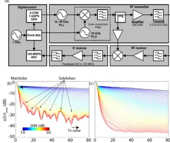
Figure 1. (a)Snow-radar hardware block diagram. Strength and location of sidelobes in the system impulse response(b)before and(c)after deconvolution of the radar data acquired during 2012 OIB Arctic campaign. Family of curves shows dependence on peak-signal-to-noise ratio (PSNR in dB) and is constructed using all the radar echoes (∼4×106)from the campaign. Normalized returns are for every 1 dB increment of PSNR between 10 and 50 dB.

Ice Sheets (KU CReSIS) and other collaborators’ field pro-grams (e.g., Patel et al., 2017; Yan et al., 2017). Below, we describe the system hardware and software processing algo-rithms used to generate the resulting data products and the changes that have been incorporated throughout the evolu-tion of the system to what is used today.

2.1.1 Hardware

Since 2009, the snow-radar hardware has been modified to improve system performance in terms of wider bandwidth, improved phase linearity at faster chirp rates, increased data acquisition rates, and real-time hardware processing. Fig-ure 1 shows the system block diagram, although specific val-ues have changed throughout the various OIB deployments. The basic components include a digital system, microwave chirp generator, microwave transmitter and receiver, and in-termediate frequency (IF) receiver. The digital system gener-ates a 600–900 MHz reference chirp from the second Nyquist band of a 1 gigasample s−1DDS, which is then multiplied by a factor of 20 by the PLL to generate a 12 to 18 GHz Ku-band signal. The 12–18 GHz signal, which is typically used by the CReSIS Ku-band altimeter, is then down-converted using a mixer driven by a 10 GHz phase-locked oscillator to produce

the system’s 2–8 GHz transmit waveform. A directional cou-pler is used to replicate the chirp for the receiver. The receiver filters, amplifies, and mixes the received waveform with the replicated chirp to produce an IF signal. This IF signal con-sists of a collection of near-constant “beat” frequency com-ponents in which target delay is expressed by a simple rela-tionship as the ratio of frequency by chirp rate. The spectral purity of each component is related to the frequency linear-ity of the 2–8 GHz chirp. Deviations from a linear frequency sweep result in reduced resolution and sidelobes. Finally, the sampled IF signal is coherently integrated or stacked four to eight times.

2.1.2 Processing

The raw data recorded by the snow radar is a stream of coherently integrated intermediate frequency signals time tagged with UTC time. In some datasets, an optional digi-tal down converter (DDC) was used. The recorded data are post-processed using the following steps:

(4)

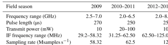
Table 1.Radar parameter used in Arctic surveys.

Field season 2009 2010–2011 2012–2015

Frequency range (GHz) 2.5–7.0 2.0–6.5 2.0–8.0

Pulse length (µs) 270 250 250

Transmit power (mW) 10 20–100 100

IF frequency range (MHz) 29.2–58.32 31.25–62.50 62.50–125.00

Sampling rate (Msamples s−1) 58.32 62.5 125

reduce range sidelobes. Additionally, any DDC-induced modifications to coherent noise components must be compensated.

2. Coherent noise removal: there are several unwanted co-herent components within the system resulting in noise signals that vary slowly with respect to time. These sig-nals are estimated by analyzing the Doppler compo-nents of the data and then removed.

3. Platform altitude and position corrections: precision GPS and inertial measurement unit information is used to position the antennas along the flight track. Relative altitude variations of the antennas within the coherent averaging window are corrected so that the subsequent coherent averaging focuses the along-track beam pat-tern towards nadir.

4. Windowing/deconvolution: phase and amplitude non-linearities of the system are estimated by analyzing data collected over specular returns produced by sea ice leads. A catalog of these responses is saved during a campaign and used to deconvolve nonlinearities to pro-duce low sidelobe waveforms. Figure 1 illustrates the effectiveness of the deconvolution process in suppress-ing sidelobes (noted in Kwok and Haas, 2015) for data collected during the 2012 OIB Arctic campaign. 5. Coherent/incoherent integration: finally, additional

co-herent and incoco-herent integrations are used to improve signal-to-noise ratio (SNR), along-track resolution, and to reduce speckle.

2.2 Snow depth from field surveys

Coordinated surveys of field measurements and OIB over-flights occurred in 2 years (2012 and 2014) under the aus-pices of two different programs. Both were located on land-fast ice to minimize to the variability introduced by the spa-tial mismatch of the airborne and ground-based measure-ments due to ice drift. A brief description of these field pro-grams is provided below.

2.2.1 BROMEX 2012

In coordination with OIB, in situ snow data were collected as part of the 2012 BROMEX (BRomine, Ozone, and

Mer-cury EXperiment) near Barrow, Alaska (Nghiem et al., 2013; Webster et al., 2014). Field measurements were conducted on smooth, first-year sea ice on Elson Lagoon, a location where landfast ice undergoes little deformation. Following the OIB pass on 15 March 2012, snow depths were measured every 1–5 m in a two-dimensional layout along two transects us-ing a GPS-enabled Magna probe unit (Sturm and Holmgren, 1999); the probe has an accuracy of 0.3 cm over level sea ice and snow (Sturm et al., 2006). The first transect (used here) consisted of three lines∼1000 m in length, each 5 m apart, for a width of 10 m. Snow density was measured ev-ery∼100 m with a Federal Sampler (Marr, 1940); the av-erage density was 306±91 kg m−3. More information about the in situ data and field conditions is available in Webster et al. (2014).

2.2.2 Eureka 2014

During March and April of 2014, a coordinated flight and field-based campaigns (sponsored by Environment and Climate Change Canada) were carried out near Eureka, Nunavut, Canada, to evaluate OIB estimates of snow depth on landfast first-year ice (FYI). A predetermined set of 11 parallel OIB flight lines was executed within Eureka Sound, a large inlet separating Axel Heiberg and Ellesmere islands, on 25 March 2014. A spacing of 12 m between OIB flight lines ensured strong coincidence between the narrow swath of the snow radar and the point-based nature of the planned field measurements. Snow depths within the radar footprints were sampled after the overflights. An extended description of the 2014 Eureka study site and field campaign can be found in King et al. (2015).

(5)

the ESC-30 (Eastern Snow Conference 30 cm cross-section corer). Extracted cores were weighed in situ with a hanging scale to estimate bulk snow density and its water equivalent. The observed snow layer along the 2014 Eureka transect was shallow, with a mean snow depth of 17.8±9.9 cm. This general condition corresponded with spatial predominance of large undeformed FYI pans (62 % of ice regions under flight of the Eureka mission). Here, smooth ice topography and sustained Arctic winds allowed rapid redistribution of snow accumulation and limited mean depths to 16.0±8.3 cm. In-creased snow depth was associated with local regions of de-formed ice where drifted accumulation was found in prox-imity to convergence features (i.e., rafting, rubble, and pres-sure ridging). Those areas were described as deformed FYI in King et al. (2015) and were shown to have a higher mean depth of 20.7±11.4 cm. Transect variations in density were conservative, with a mean of 306 kg m−3_{and standard}

devi-ation of 50 kg m−3_{, which is comparable to the assumed}

cli-matological mean of∼320 kg m−3near the end of the win-ter.

2.3 Snow depth from snowfall and climatology

Averaged retrievals (25 km×25 km) from the five algo-rithms are compared with both snow depths from snowfall in ERA-Interim products and a modification of the W99 clima-tology. We elected to use the ERA-Interim products here be-cause it is one of the more broadly used reanalysis in climate work and compares reasonably with the modified climatol-ogy (see Sect. 4). Below, the procedures for constructing these daily fields of basin-wide snow depths are described.

2.3.1 Snow depth from ERA-Interim snowfall (ERAI-sf)

Fields of snow depth from ERA-interim snowfall are con-structed following Kwok and Cunningham (2008). Daily snowfall on ice parcels (100 km×100 km) across the Arc-tic Ocean is recorded on a daily basis. Ice drift is from op-timally interpolated motion fields (described in Kwok et al., 2013). A daily cycle of accumulation and ice advection is carried out for each Lagrangian parcel, which mimics the process of snow accumulation over sea ice in motion. Start-ing from 15 August, the snowfall on each driftStart-ing parcel is recorded and accumulated through the end of spring. Surface conditions (air temperature and ice concentration) determine when and where snow is allowed to accumulate. Accumula-tion is permitted only when the ERA-Interim 2 m air temper-ature is below freezing and the AMSR-E ice concentration exceeds 50 %. When ice concentration drops below 50 %, the accumulated snow is removed from that parcel. As ice con-centrations rarely drop below 50 % within the perennial ice pack, this condition is only relevant to the accumulation pro-cess over seasonal ice during the advance of the ice cover in the fall. Typically, the snow is thinner where the ice cover

is formed later in the season (W99; Sturm et al., 2002; Web-ster et al., 2014). The snow density climatology of Kwok and Cunningham (2008) (a modified version of that used in W99) is used to convert snow water equivalent into snow depth. No initial snow cover, representing snow that survived the melt season, is added to the multiyear ice at the beginning of the accumulation season. Henceforth, we refer to snow depth from this procedure as ERAI-sf estimates.

2.3.2 Snow depth from modified climatology (modW99)

In this paper, we compute snow depth (hfs)from the

clima-tology (W99) following Kwok and Cunningham (2015) as

hs(X, t, fFY)=hWs (X, t )(1−fFY)+αhWs (X, t )fFY.

We use the annual space-varying snow depth and density,

hW_s (X, t ), from the snow climatology in W99. We note that this W99 climatology is from in situ data collected between 1954 and 1991, and it is considered to be representative of snow depth over multiyear ice, so it does not address the snow depth over the seasonal ice cover of the Arctic Ocean. To account for reduced snow depth over FYI, we follow Laxon et al. (2013), who used a fraction (α)of the climato-logical snow depth to represent the reduced snow accumula-tion over FYI identified by Kurtz and Farrell (2011). Herehs

is dependent on the fractional coverage of FYI (fFY), derived

from ASCAT scatterometer data (following Kwok, 2004). The fFY retrievals from ASCAT impart time-varying

spa-tial patterns upon these otherwise static climatological fields. While Laxon et al. (2013) used a fixed value ofα=0.5, here we useα=0.7, based on a subsequent analysis of CryoSat-2 ice thickness (Kwok and Cunningham, CryoSat-2015). Since the above construction represents a modification of the W99 climatology, we henceforth refer to these snow depths as modW99 estimates.

2.4 Retrieval algorithms

Five sets of retrievals from five separate algorithms are con-sidered here. The first algorithm below produced the standard product (2009–2013) that is archived at and distributed by the National Snow and Ice Data Center (NSIDC). The remaining algorithms were developed by members of the Snow Thick-ness On Sea Ice Working Group. Only brief summaries of each algorithm are provided here, and the reader is referred to the published literature for details on each of the algorithms. These retrieval algorithms differ in the way the air–snow and snow–ice interfaces are detected and localized in the radar returns. Figure 2 shows the different range locations of the interfaces in a collection of radar returns from Eureka; these differences are discussed in Sect. 3.5.

(6)

Eureka 20140325 02 069

10

20

30

40

50

60

70

80

Range bin

50 100 150 200

Snow-ice interface

Air-snow

interface

Ra

d

ar

10

20

30

40

50

60

70

80

Range bin

-30 -20 -10 0 10 20

Return power (dB)

(b) (a)

Power

GSFC-NK SRLD

Wavelet JPL

Snow radar record

Figure 2.Location of the air–snow and snow–ice interfaces overlaid on power of return echoes.(a)Examples from four algorithms (black trace denotes the air–snow interface; blue trace denotes the snow–ice).(b)Except for the modeled GSFC-NK algorithm, the variability in the interface locations (e.g., leading edge, peak) depends on the algorithm.

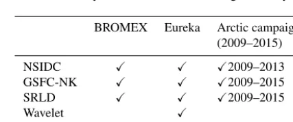
it does not include all relevant algorithms (e.g., Holt et al., 2015). Table 2 shows the datasets that were available and used herein.

2.4.1 Existing NSIDC product (NSIDC)

This algorithm was used for the Sea Ice Freeboard, Snow Depth, and Thickness data product that is archived at NSIDC with the following designation: IDSI4 (Kurtz et al., 2015). Details of the full algorithm methodology are described in Kurtz et al. (2013). Briefly, the algorithm is an empirical method that selects the a–s interface using a combined peak and threshold method. The a–s interface is taken to be ei-ther the first significant peak above a defined threshold or the first point when the rise in the radar return reaches a speci-fied threshold if no peak is found. The method uses a linear scaling relation for the first version of the snow-radar data collected in 2009 to select the thresholds used in the algo-rithm (as described in Kurtz and Farrell, 2011). The location of the s–i interface is defined as the maxima in the radar sig-nal below the a–s interface.

2.4.2 GSFC-NK

The GSFC-NK algorithm was used for the process-ing of quick-look IceBridge data in 2014–2016 (https: //nsidc.org/data/docs/daac/icebridge/evaluation_products/

Table 2.Availability of retrieval datasets during this study.

BROMEX Eureka Arctic campaigns (2009–2015)

NSIDC X X X2009–2013

GSFC-NK X X X2009–2015

SRLD X X X2009–2015

Wavelet X

JPL X X X2009–2015

sea-ice-freeboard-snowdepth-thickness-quicklook-index. html). Full details of the algorithm methodology are described in the product documentation at NSIDC. The algorithm is a waveform fitting method that follows the algorithm used for CryoSat-2 surface height retrievals described by Kurtz et al. (2014). A modification to that al-gorithm accounts for the different instrument characteristics of the snow radar and accounts for coherent scattering of the return using a heterogeneous flat patch surface model (Brown, 1982). The algorithm fits a model waveform to the snow-radar data using a bounded trust region method (Coleman and Li, 1996). Both the a–s and s–i interfaces are selected from the model fit results.

(7)

between the processing time needed and the quality of the fit obtained. The most important of these parameters are the ini-tial guess and model fit bounds for the a–s and s–i interfaces along with the maximum number of iterations used in the fitting process. The initial guesses for the interface locations are taken from the empirical algorithm of the existing NSIDC product, and the bounds for the possible interface locations are restricted to be within±1.5 ns of the initial guesses. The maximum number of fit iterations was set to 300. Due to the large processing time needed for the algorithm, it was run on every other point for this comparison. The model fit qual-ity was determined by calculating the sum of the waveform power divided by the squared norm of the fit residual, and fits with a value less than 0.2 were discarded.

2.4.3 SRLD

The Snow Radar Layer Detection (SRLD) algorithm was first developed for layer detection on land ice, in which the de-tection of the a–s interface and s–i interface is determined prior to the subsequent detection of deeper layers within the firn (Koenig et al., 2016). Over sea ice, only the a–s and s–i interfaces are returned by the algorithm. The initial appli-cation to existing OIB snow-radar data from various cam-paigns (2009–2012) and the need for it to be applicable to future campaigns required a process that would adapt to the data and not be dependent on fixed thresholds in the radar re-turn signal. The SRLD method uses the gradient between the open-air return values and the maximum return value to lo-cate the two interfaces. The a–s interface is taken to be where the presence of snow has caused the radar return level to be elevated above the open-air values, near the beginning of the gradient. The s–i interface is taken to occur where the transi-tion from snow to ice has produced a maximum peak in radar return level – at the end of the gradient. The open-air value is first determined by taking a sample median of the values above the surface for the data frame being analyzed. The me-dian of the peak values is used, along with the open-air value, to define the gradient to which a threshold is then applied for the determination of the a–s interface. These gradient end-points, comprised of the median air value and median peak value, adjust with the data from frame to frame. In the cur-rent implementation, the midpoint radar power level is used as the threshold. The point at which this radar power level maps onto each radar return profile determines the a–s in-terface, while the peak level in the return determines the s–i interface.

2.4.4 Wavelet

The Wavelet algorithm, described by Newman et al. (2014), operates on each trace (column) of an echogram indepen-dently and has three components: interface detection through the use of the Haar wavelet–continuous wavelet transform (Haar-CWT), topographic filtering using the htopo

parame-ter (to mitigate against heavily deformed ice topography on the radar point of closest approach), and the assignment of precision to each derived snow depth using radar system pa-rameters.

The Haar-CWT is optimized for detecting abrupt transi-tions within a signal, such as those arising from interface returns, with the largest Haar-CWT coefficients localized at the largest magnitude signal transition. To detect the a–s and s–i interfaces, the echograms were preconditioned in differ-ent ways. To detect the a–s interface the logarithm of the echogram results in the largest magnitude signal transition occurring at the a–s interface. To detect the s–i interface the echogram is left in its original form, wherein the largest mag-nitude signal transition occurs at the s–i interface. The Haar-CWT is then applied to each echogram trace and the result-ing coefficients are summed over a range of different scales – from the broad localization of the interface at large wavelet scales to precise localization at small wavelet scales. The in-terface location is assigned to the location of the maximum of the summed coefficients. The benefits of this algorithm are that (1) it is robust and does not depend on a set of fixed thresholds and (2) the interface detection process is not af-fected by changes in transmitted power and receiver noise, which vary both during and between different OIB flight campaigns.

Interface picks associated withhtopo values greater than

50 cm are ignored as they are associated with heavily de-formed ice topography, such as sea ice pressure ridges, where derived snow depths have been shown to be unreliable due to uncertainty in the radar scattering surface. Interface picks associated withhtopo values of less than 50 cm are deemed

valid and converted to snow depth by considering two-way travel time in the snow pack and the permittivity of snow.

Derived snow depths are assigned a precision based upon concurrent snow-radar system parameters. Snow depth preci-sion is calculated for each derived snow depth independently, with the final precision value the sum of terms relating to the SNR at the a–s interface, the signal-to-clutter ratio at the s–i interface, the fast-time range bin spacing, and the bandwidth-dependent range resolution of the snow radar.

2.4.5 JPL

This is a simplified version of the algorithm by Kwok and Maksym (2014) that deals with residual system sidelobes in the returns. Since a reprocessed version of the radar dataset with suppressed system sidelobes is now available for all years except 2013, this aspect of the algorithm has been dis-abled.

(8)

0 2 4 6 8 10 12 14 Snow depth standard deviation (cm)

1872 samples Mean/SD: 6.14 ± 1.51 cm Mean/SD: 2.24 ± 1.21 cm

pdf (/cm)

33 409 samples Mean/SD: 7.11 ± 3.68 cm Mean/SD: 1.90 ± 1.64 cm

0 5 10 15 20 25 30

Snow depth standard deviation (cm)

pdf (/cm)

(a)

(b)

0 5 10 15 20 Distance (m) 0.0 0.2 0.4 0.6 0.8 1.0 Correlation 2 4 6 8 10 12 14 N observations (10 )3

0 5 10 15 20 Distance (m) 0.0 0.2 0.4 0.6 0.8 1.0 Correlation 0.5 1.0 1.5 2.0

N observations (10

)

3

0 5 10 15 20 Distance (m) 0.0 0.2 0.4 0.6 0.8 1.0 Correlation 0.5 1.0 1.5 2.0 N observations (10 )3

0 5 10 15 20 Distance (m) 0.0 0.2 0.4 0.6 0.8 1.0 Correlation 2 4 6 8 10 12 14 N observations (10 ) 3

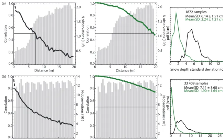
Figure 3.Spatial correlation (left and center) and variability (right panel) of snow depth measurements from(a)BROMEX and(b)Eureka before (black lines) and after (green lines) averaging (diameter of 40 m). Gray bars show the number of measurements used in each correlation calculation. Pdf is probability density function.

system bandwidth controls the width (or sharpness) of a lo-cal maximum and the rate of rise of its leading edge. The al-gorithm uses these system-dependent parameters to adapt to the changes in the radar system as the bandwidth and noise level of the snow radar have progressively improved over the course of the OIB mission. The highest significant peak in the echo profile is designated as the return from the s–i interface. Returns from a–s interfaces are assumed to be weaker and are the first significant range returns, determined using the above criteria, above the s–i interface. Once the interfaces are detected, the radar range to the interface is localized in an oversampled (by 16 times) version of the echo return; this reduces the range error in the identification of the local max-ima in the echo return. From a scattering perspective, this restricts the detected returns to a–s interfaces that are more specular and appear as a detectable peak, rather than just the strength of the leading edge.

3 Comparisons with field surveys

In this section, we first describe the comparison approach and the expected variability of the differences given the statis-tics of the retrievals and field measurements. Next, results from comparisons with measurements from BROMEX and Eureka are discussed. Lastly, we contrast the absolute range locations of the a–s and s–i interfaces from the different al-gorithms, which provides insights into the preferred location on the echo profile that each algorithm designates as an

in-terface. To account for the reduced propagation speed of the radar wave in the snow layer, all radar measurements below were converted to snow depth, assuming an end-of-winter bulk density of 320 kg m−3(W99); snow depth estimates are relatively insensitive to uncertainties in bulk density (see er-ror estimates in Kwok et al., 2011).

3.1 Comparison approach

(9)

600 620 640 660 680 700 720 10 20 30 40 50

Snow depth (cm)

600 620 640 660 680 700 720 Snow-radar record 10 20 30 40 50

Snow depth (cm)

600 620 640 660 680 700 720 10

20 30 40 50

Snow depth (cm)

10 20 30 40 50

10 20 30 40 50 R: 0.44 113 samples

Diﬀ: -4.82 ± 3.98 cm

10 20 30 40 50

BROMEX snow depth (cm) 10 20 30 40 50 R: 0.67 169 samples

Diﬀ: -1.81 ± 3.36 cm

10 20 30 40 50

10 20 30 40 50 R: 0.66 227 samples

Diﬀ: 4.15 ± 3.35 cm

0 2 4 6 8 10 12 14

pdf (/cm)

0 2 4 6 8 10 12 14

pdf (/cm)

Snow depth standard deviation (cm)

0 2 4 6 8 10 12 14

1079 samples Mean/SD:10.69 ± 7.28 cm Mean/SD: 2.34 ± 1.80 cm

pdf (/cm)

Snow depth (cm)

10 20 30 40 50

Snow depth (cm)

600 620 640 660 680 700 720

0 2 4 6 8 10 12 14 10 20 30 40 50

R: 0.54 227 samples Diﬀ: 0.29 ± 4.17 cm

10 20 30 40 50

Snow depth (cm)

pdf (/cm)

(a) (b) (c) (d) NSIDC GSFC-NK JPL SRLD Before averaging After averaging Radar retrievals Field measurements Radar retrievals Field measurements Radar retrievals Field measurements Radar retrievals Field measurements

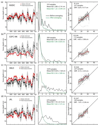
Figure 4.Comparison of four algorithms with field measurements from BROMEX:(a)NSIDC,(b)GSFC-NK,(c)SRLD, and(d)JPL. Left panel: averaged field (black dots) and retrieved (red dots) snow depths with standard deviation at each sample (gray band). Center panel: standard deviation of retrieved snow depth before (black) and after (green) averaging−40 m along track. Right panel: scatterplot shows correlation (R) between the averaged snow depth samples; the number of samples and the mean and standard deviation of the differences are shown on the top-left corner of plot. Error bars show standard deviation of samples in 2 cm bins.

within a 20 m circle reduced from 6.1±1.5 to 2.2±1.2 cm and for the Eureka data from 7.1±3.7 to 1.9±1.6 cm.

To compare the averaged measurements (at a 40 m spac-ing), we take the difference between the estimates of the snow radar (dsr)and field (df)as1d=dsr−df. Assuming

that these two estimates are random variables that are un-correlated and normally distributed, the variance of 1d is expected to beσ_1d2 =σ_sr2+σ_f2. The contribution ofσfis

ex-pected to be bounded by the values in the distribution shown in Fig. 2, and the contribution ofσsris discussed below. With

the bounds on the two expected variances,σ1d can be esti-mated for assessment of their differences.

3.2 Comparisons with snow depth from BROMEX

(10)

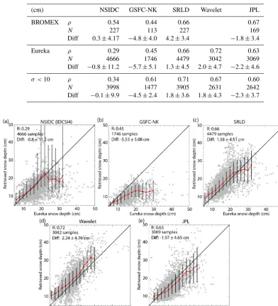
Table 3.Comparison of averaged radar snow depth with field measurements at BROMEX and Eureka. The additional comparisons at Eureka are for samples where the standard deviation of the field-measured snow depth within the averaging radius of 20 m is less than 10 cm.

(cm) NSIDC GSFC-NK SRLD Wavelet JPL

BROMEX ρ 0.54 0.44 0.66 0.67

N 227 113 227 169

Diff 0.3±4.17 −4.8±4.0 4.2±3.4 −1.8±3.4

Eureka ρ 0.29 0.45 0.66 0.72 0.63

N 4666 1746 4479 3042 3069

Diff −0.8±11.2 −5.7±5.1 1.3±4.5 2.0±4.7 −2.2±4.6

σ <10 ρ 0.34 0.61 0.71 0.67 0.60

N 3998 1477 3905 2631 2642

Diff −0.1±9.9 −4.5±2.4 1.8±3.6 1.8±4.3 −2.3±3.7

Figure 5.Comparison of five algorithms with field measurements from Eureka:(a)NSIDC,(b)GSFC-NK,(c)SRLD,(d)Wavelet, and

(e)JPL. Scatterplot shows correlation (R) between the averaged snow depth samples; the number of samples and the mean and standard deviation of the differences are show on the top-left corner of plot. Error bars show standard deviation of samples in 2 cm bins.

30 cm. Except for the mean differences, it is apparent that the along-track variability in snow depth is reproduced rea-sonably well, as measured by the correlations between the radar and field estimates (0.45–0.67). Of note is the lower scatter and reduced sample size in the distributions of σsr

for both the NSIDC and GSFC-NK retrievals prior to av-eraging (Fig. 4). This pattern can be attributed to the fact that both these algorithms used averaged waveforms in their retrievals, rather than raw waveforms provided in the radar data, and thus the data have already been smoothed and sub-sampled before the retrieval process. The averaging of the

SRLD and JPL retrievals, in contrast, reducedσsrby a factor

of∼5. In any case, the standard deviation of the differences of∼3–4 cm (Fig. 4) is approximately what one would expect when calculating (σ_1d2 =σ_sr2+σ_f2)using the values ofσfin

Fig. 2a and values ofσsrin Fig. 4 (center panels). In these

(11)

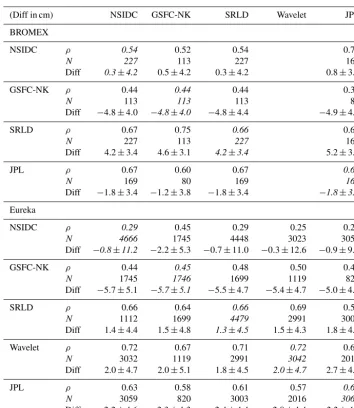
Table 4.Comparison of radar snow depth with field measurements at BROMEX and Eureka using retrievals at locations that are common to both algorithms. In the matrix presentation below, the snow depth retrieved by the row algorithm (at locations common to the column algorithm) are used in the comparisons with field data. Note that the matrix is not symmetric. Quantities in italics are from Table 3.

(Diff in cm) NSIDC GSFC-NK SRLD Wavelet JPL

BROMEX

NSIDC ρ 0.54 0.52 0.54 0.70

N 227 113 227 169

Diff 0.3±4.2 0.5±4.2 0.3±4.2 0.8±3.0

GSFC-NK ρ 0.44 0.44 0.44 0.39

N 113 113 113 80

Diff −4.8±4.0 −4.8±4.0 −4.8±4.4 −4.9±4.5

SRLD ρ 0.67 0.75 0.66 0.68

N 227 113 227 169

Diff 4.2±3.4 4.6±3.1 4.2±3.4 5.2±3.2

JPL ρ 0.67 0.60 0.67 0.67

N 169 80 169 169

Diff −1.8±3.4 −1.2±3.8 −1.8±3.4 −1.8±3.4

Eureka

NSIDC ρ 0.29 0.45 0.29 0.25 0.28

N 4666 1745 4448 3023 3059

Diff −0.8±11.2 −2.2±5.3 −0.7±11.0 −0.3±12.6 −0.9±9.5

GSFC-NK ρ 0.44 0.45 0.48 0.50 0.46

N 1745 1746 1699 1119 820

Diff −5.7±5.1 −5.7±5.1 −5.5±4.7 −5.4±4.7 −5.0±4.2

SRLD ρ 0.66 0.64 0.66 0.69 0.59

N 1112 1699 4479 2991 3003

Diff 1.4±4.4 1.5±4.8 1.3±4.5 1.5±4.3 1.8±4.1

Wavelet ρ 0.72 0.67 0.71 0.72 0.67

N 3032 1119 2991 3042 2016

Diff 2.0±4.7 2.0±5.1 1.8±4.5 2.0±4.7 2.7±4.4

JPL ρ 0.63 0.58 0.61 0.57 0.63

N 3059 820 3003 2016 3069

Diff −2.2±4.6 −2.3±4.3 −2.4±4.4 −2.0±4.4 −2.2±4.6

3.3 Comparisons with snow depth from Eureka

The comparisons with Eureka field measurements are shown in Fig. 5 and the results are summarized in Table 3. This com-parison includes many more samples from the multiple OIB tracks and more extensive sampling of the surface compared to the BROMEX survey. Averaged snow depth ranges from

∼5 cm to more than 45 cm. This richer dataset tests the skill of five algorithms over a broad range of snow depths. Vari-ability is between 0.29 and 0.72, as measured by the corre-lations between the radar and field estimates. The NSIDC and GSFC-NK algorithms have lower correlations, as their retrievals tend to underestimate snow depth; these two algo-rithms seem to be insensitive to snow depths that are more than∼20 cm in this case. The SRLD, Wavelet, and JPL

re-trievals have comparable correlations (0.66–0.72) with field data. Broadly, these algorithms tend to overestimate snow depths below∼10 cm, with higher variability in retrievals over thicker snow (Fig. 5). Except for the NSIDC retrievals, the standard deviation of the differences of∼4–5 cm is ap-proximately as expected when calculated using the values of

σfin Fig. 2b and values of σsr (σ1d2 =σsr2+σf2; not shown

here). In these comparisons, the mean differences vary be-tween a maximum of−6 cm (GSFC-NK) and a minimum of

−1 cm (NSIDC).

We also examined the impact of surface roughness on the quality of the retrievals from the different algorithms (Ta-ble 3). We define roughness asσf, as defined above and as

(12)

rough-ness >10 cm were not included in the comparisons, there would be a consistent decrease in the standard deviation of the differences for all retrievals. This suggests that all the retrievals seem to be affected by surface roughness, consis-tent with the results reported by King et al. (2015). How-ever, the correlation values did not increase for all algorithms (NSIDC: 0.29 to 0.34; GSFC-NK: 0.45 to 0.61; SRLD: 0.66 to 0.71; Wavelet: 0.72 to 0.67; JPL: 0.63 to 0.60).

3.4 Algorithm-dependent filtering strategies: BROMEX and Eureka

For both the BROMEX and Eureka comparisons, the dif-ferent algorithms do not provide the same number of re-trievals (Table 3) because of algorithm-dependent filtering strategies for removing low-quality estimates. More conser-vative strategies reduce the retrieval rate, which may bias these comparisons. We address this concern by examining the retrieval results for only those samples that are common to a pair of algorithms. Table 4 shows the results from all pairings of the five algorithms. Broadly, the changes in the comparison measures (i.e.,ρand “Diff”) did not change sig-nificantly for both BROMEX and Eureka. Compared to the diagonal element of the matrices in Table 4, the mean differ-ences and standard deviations (relative to the field data) re-main similar even when only the subset of common samples was used. Hence, we conclude that the statistics in Table 3 are fairly robust measures of the retrievals and relatively in-sensitive to the filtering strategies devised.

3.5 Different approaches to localize the air–snow and snow–ice interfaces

As observed earlier, the comparisons show that the biases (or mean differences) for individual algorithms are consistent (similar in magnitude) at both BROMEX and Eureka. For ex-ample, the mean differences of the SRLD and JPL retrievals are approximately+2 and−2 cm, respectively, at both field sites (see Table 3). Thus, on average, the SRLD snow depth retrievals are 4 cm higher than the JPL retrievals. These pat-terns suggest that systematic biases exist within individual algorithms due to their range determinations of the a–s and s–i interfaces in the echograms. In each retrieval algorithm, a particular characteristic of a leading edge (see Fig. 3b) or return peak is typically used to determine the range point to be the location of an interface. In this case, the same charac-teristic has to be used consistently for both the a–s and s–i interfaces, otherwise the range distance between the two in-terfaces will be biased.

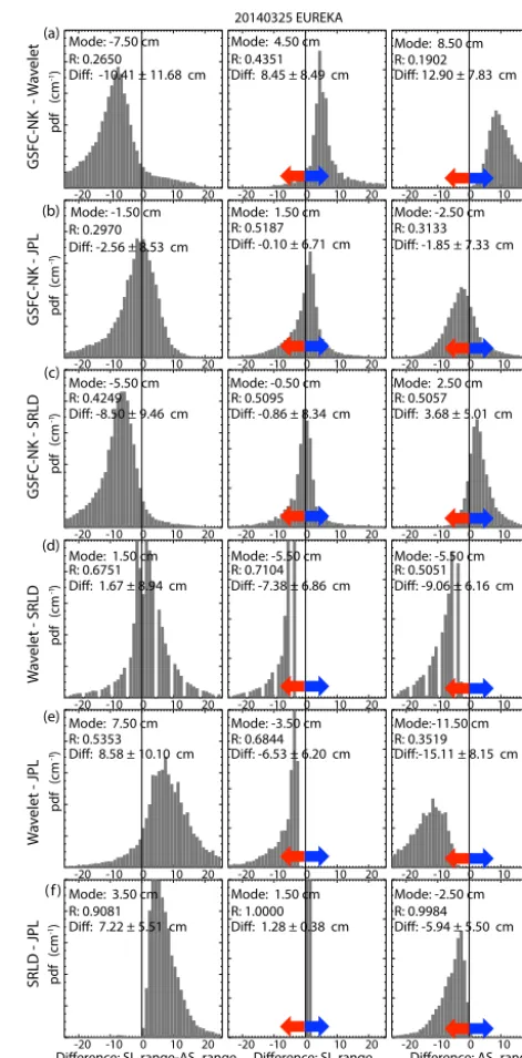
Here, we compare the range locations of the two interfaces selected by four of the five algorithms to assess the contribu-tion of algorithm-induced biases seen in the observed mean differences at the Eureka site (Fig. 6). The left panel (Fig. 6) shows whether there are mean differences in the retrieved range distances (calculated from the range locations of the

20140325 EUREKA

-20 -10 0 10 20 -20 -10 0 10 20

-20 -10 0 10 20

-20 -10 0 10 20 -20 -10 0 10 20

-20 -10 0 10 20

SRLD - JPL

W

av

elet - JPL

GSFC-NK - SRLD

GSFC-NK -

W

av

elet

GSFC-NK - JPL

W

av

elet - SRLD

Difference: SI_range Difference: AS_range Difference: SI_range-AS_range Far range Near range pdf (cm ) -1 pdf (cm ) -1 pdf (cm ) -1 pdf (cm ) -1 pdf (cm ) -1 pdf (cm ) -1

Mode: 4.50 cm Mode: 8.50 cm

Mode: 1.50 cm Mode: -2.50 cm

Mode: -5.50 cm Mode: -5.50 cm

Mode: 2.50 cm

Mode: -3.50 cm Mode:-11.50 cm

Mode: 7.50 cm Mode: 1.50 cm Mode: -5.50 cm Mode: -7.50 cm

Mode: -0.50 cm R: 0.2650

Diﬀ: -10.41 ± 11.68 cm

R: 0.4351 Diﬀ: 8.45 ± 8.49 cm

R: 0.1902 Diﬀ: 12.90 ± 7.83 cm

R: 0.2970 Diﬀ: -2.56 ± 8.53 cm

R: 0.5187 Diﬀ: -0.10 ± 6.71 cm

R: 0.3133 Diﬀ: -1.85 ± 7.33 cm

R: 0.4249 Diﬀ: -8.50 ± 9.46 cm

R: 0.5095 Diﬀ: -0.86 ± 8.34 cm

R: 0.5057 Diﬀ: 3.68 ± 5.01 cm

R: 0.6751 Diﬀ: 1.67 ± 8.94 cm

R: 0.7104 Diﬀ: -7.38 ± 6.86 cm

R: 0.5051 Diﬀ: -9.06 ± 6.16 cm

R: 0.5353

Diff: 8.58 ± 10.10 cm R: 0.6844Diff: -6.53 ± 6.20 cm R: 0.3519Diff:-15.11 ± 8.15 cm

R: 0.9081

Diﬀ: 1.28 ± 0.38 cm R: 1.0000 Diﬀ: 7.22 ± 5.51 cm

R: 0.9984 Diﬀ: -5.94 ± 5.50 cm

(a)

(b)

(c)

(d)

(e)

( f )

Figure 6.Distribution of differences in range locations:(a) GSFC-NK minus Wavelet,(b)GSFC-NK minus JPL,(c)GSFC-NK mi-nus SRLD,(d)Wavelet minus SRLD,(e)Wavelet minus JPL, and

(f)SRLD minus JPL. Left panel: differences in the range between the two interfaces. Center panel: differences in radar range to the snow–ice (s–i) interface. Right panel: differences in radar range to the air–snow (a–s) interface.

(13)

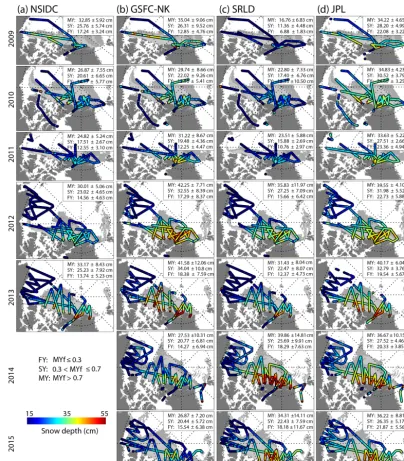
Figure 7.Seven years (2009–2015) of retrieved snow depths from four algorithms:(a)NSIDC,(b)GSFC-NK,(c)SRLD, and(d)JPL. Snow depths (top-left corner) are averages based on three categories of multiyear ice fractions (MYf) shown in legend. Background shows multiyear sea ice fraction (dark gray: MYf≥0.7; light gray: 0.3<MYf<0.7; white: MYf≤0.3). Corresponding snow depth distributions are shown in Fig. 8. The gray shadings represent regions with>0.7 (darker) and>0.9 (lighter) MYf. Repeat tracks are not shown here.

given echogram as the location of the s–i interface, so they have a narrow distribution of differences in the range loca-tion of that interface (∼1 cm). Nearly all of their difference in retrieved snow depth can be attributed to differences in the location of the a–s interfaces (Fig. 6f). The SRLD algorithm locates the a–s interface on the leading edge, while the JPL algorithm located it at the local peak following the leading edge. Relative to the JPL a–s interfaces, the SRLD a–s inter-faces are always displaced toward the radar, i.e., in the near and therefore shorter range. Thus, the range distance to the

(14)

70%

MYf ≤ 0.3 0.3 < MYf ≤ 0.7 MYf > 0.7

20 40 60 80 100

pdf (/cm)

20 40 60 80 100 20 40 60 80 100 20 40 60 80 100 20 40 60 80 100 20 40 60 80 100 20 40 60 80 100 2009

20 40 60 80 100

pdf (/cm)

2010

20 40 60 80 100 2011

20 40 60 80 100 2012

20 40 60 80 100 20 40 60 80 100 2013

20 40 60 80 100

pdf (/cm)

20 40 60 80 100 20 40 60 80 100 20 40 60 80 100 20 40 60 80 100 20 40 60 80 100 20 40 60 80 100

20 40 60 80 100 Snow depth (cm)

pdf (/cm)

20 40 60 80 100 20 40 60 80 100

Snow depth (cm)20 40 60 80 100 20 40 60 80 100Snow depth (cm)20 40 60 80 100 20 40 60 80 100

2014 2015 NSIDC GSFC-NK SRLD JPL (a) (b) (c) (d)

12.9 ± 4.8 26.3 ± 9.5 35.0 ± 9.1

12.5 ± 5.4 22.0 ± 9.3 29.7 ± 8.7

12.3 ± 4.5 19.5 ± 4.4 31.2 ± 8.7

17.3 ± 8.4 32.6 ± 8.4 42.3 ± 7.7

18.4 ± 7.6 34.0 ± 10.9 41.6 ± 12.1

14.3 ± 6.9 20.8 ± 6.8 27.5 ± 10.3

15.5 ± 6.4 20.4 ± 5.7 26.9 ± 7.2 17.2 ± 3.2

25.8 ± 5.7 32.9 ± 5.9

14.1 ± 5.8 20.6 ± 6.7 26.9 ± 7.6

12.6 ± 3.1 17.5 ± 2.7 24.8 ± 5.2

14.6 ± 4.6 23.0 ± 4.7 30.0 ± 5.1

13.7 ± 5.2 25.2 ± 7.9 33.2 ± 8.4

6.9 ± 1.8 11.4 ± 4.5 16.8 ± 6.8

12.3 ± 10.5 17.4 ± 6.8 22.8 ± 7.3

10.8 ± 3.0 15.9 ± 2.7 23.5 ± 5.9

15.7 ± 6.4 27.3 ± 7.1 35.8 ± 12.0

12.4 ± 4.7 22.5 ± 8.1 31.4 ± 8.0

18.3 ± 7.6 25.7 ± 9.9 39.9 ± 14.8

18.2 ± 11.7 22.4 ± 7.6 34.3 ± 14.1

22.1 ± 3.2 28.2 ± 5.0 34.2 ± 4.7

24.7 ± 3.3 30.5 ± 3.8 34.8 ± 4.2

23.4 ± 4.9 27.5 ± 2.7 33.6 ± 5.2

22.7 ± 5.9 32.0 ± 5.5 39.6 ± 4.1

19.5 ± 5.7 32.8 ± 3.8 40.2 ± 6.0

20.3 ± 3.9 27.5 ± 4.5 36.7 ± 10.2

21.9 ± 5.6 26.4 ± 5.2 36.2 ± 8.8

Figure 8.Snow depth distributions in 7 years (2009–2015) of retrievals:(a)NSIDC,(b)GSFC-NK,(c)SRLD, and(d)JPL. Quantities on top-right corners are the mean and standard deviation of the sample populations in three multiyear/seasonal ice regimes (MYf≥0.7; 0.3<MYf<0.7; MYf≤0.3).

4 Basin-scale assessments

We next assess the retrieved OIB snow depths from all Arc-tic campaigns at a longer averaging length scale (>10 km). First, we summarize the overall retrievals from four al-gorithms available for this analysis (NSIDC, GSFC-NK, SRLD, and JPL). Second, the consistency of retrievals at crossovers and repeat tracks (12.5 km) is examined. Last, we compare the averaged retrievals (at 25 km) with the fields of snow depth constructed from ERA-Interim snowfall and modified climatology (modW99). These large-scale compar-isons provide a broad assessment of the spatial and interan-nual variability of the snow-radar retrievals, along with their relative agreement with the two reconstructed fields of snow depth.

4.1 Summary of basin-scale snow depths: 2009–2015

Figure 7 shows 7 years (2009–2015) of retrievals (25 km av-erages) from four algorithms (NSIDC, GSFC-NK, SRLD, and JPL). These maps show the spatial differences in the re-trievals from all the OIB flight tracks for a particular Arctic campaign. Figure 8 shows the associated snow depth distri-butions in three multiyear/seasonal ice regimes (MYf≥0.7; 0.3<MYf<0.7; MYf≤0.3), where MYf is the fraction of multiyear sea ice, MYI, coverage within each 25 km sample. The calculated mean and standard deviation of the sample population of snow depth in each of the three categories are shown on the top-left corner of each panel.

As seen in the spatial maps and distributions (Figs. 7 and 8), the snow depth within the MYI cover north of Greenland and next to the Canadian Arctic Archipelago is highest in all

the retrievals. In general, the average snow depth over the seasonal ice is thinner than those within the MYI cover. Of note is that the snow depth in the southern Beaufort Sea is always the thinnest, especially for those tracks between 2012 and 2015. The differences in retrievals from the four algo-rithms are examined in more detail in Sect. 4.3.

4.2 Comparisons at crossovers and repeat tracks

(15)

Figure 9.Differences of snow depth retrievals at crossovers and repeat tracks.(a)Crossovers with varying time separation. Mean and standard deviation of differences and correlation coefficients (R) are shown on each plot.(b)Repeat tracks: 2 April 2010, 5 April 2010, 17 March 2011, and 22 March 2012. Inset shows the distribution of differences and quantities show mean and standard deviation of differences, correlation, and sample population. Each sample represents the mean snow depth in a 4 km along-track segment. (Note: on 21 April 2009, the snow radar was operated with an altitude difference of∼300 m in the outbound and return tracks.)

Figure 9b compares the snow depth at four available re-peat tracks. These near-exact rere-peat tracks are of outbound and return segments flown during the same flight, so the time separations are typically less than a few hours. Except for ice drift, the snow radar should be acquiring data over similar snow and ice conditions. The difference distributions show that the mean differences are at most∼2–3 cm. The sign and magnitude of the differences are consistent across all the re-trievals and suggest that these are valid mean differences in the estimated snow depth. These comparisons also suggest that even though the algorithms produce self-consistent re-sults, the mean snow depth can be quite different between the algorithms, as is evident in the difference in retrieved snow depths from the four algorithms (Fig. 9b).

4.3 Comparisons with snow depth from ERA-Interim snowfall (ERAI-sf) and modified climatology (modW99)

The snow depth estimates from ERAI-sf, modW99, and their differences along OIB flight tracks are shown in Fig. 10a. The large-scale patterns are similar to the thinner snow over seasonal ice and thicker snow in regions with higher MYf, especially north of Greenland and the Canadian Arctic Archipelago. Relative to the modW99 estimates, the ERAI-sf snow depths are broadly lower over the entire Arctic Ocean ice cover, except in 2012.

(16)

clima-Figure 10.Comparison of snow depth from ERAI-sf and modW99 climatology at the snow-radar tracks:(a)ERAI-sf,(b)modW99, and

(c)difference between(a)and(b). The mean and standard deviation in each of the three categories of MYf are shown on the top-left corner of each panel.

tology (W99) and are modulated by only the timing of the OIB flights and spatial variability of MYf derived from satel-lite data. The largest differences can be seen in the southern

(17)

ad-15 20 25 30 35 40 45

10 15 20 25 30 35 40

5 10 15 20 25 30 35

2009 2010 2011 2012 2013 2014 2015 2009 2010 2011 2012 2013 2014 2015 2009 2010 2011 2012 2013 2014 2015 2009 2010 2011 2012 2013 2014 2015

NSIDC GSFC-NK SRLD JPL

Sn

ow

de

pt

h (

cm

)

Year

modW99 ERAI-sf Snowradar

MYf ≤ 0.3 0.3 < MYf ≤ 0.7

MYf > 0.7

Figure 11.Comparison of snow depth retrievals from four algorithms (NSIDC, GSFC-NK, SRLD, JPL) with ERAI-sf and modW99 estimates in three multiyear/seasonal ice regimes (MYf≥0.7; 0.3<MYf<0.7; MYf≤0.3).

vected into this region, which was used in the construction of the modW99 fields but is absent in the ERAI-sf fields (be-cause the MYf is not used in the estimates). Away from the coastal zones and away from the transition zone between the MYI and seasonal ice cover, these differences are less pro-nounced.

Figure 11 also shows the IAV in the mean snow depth from the four algorithms. Three of the algorithms (NSIDC, GSFC-NK, and SRLD) have relatively large IAV compared to the two constructed fields. In the mean, the NSIDC snow depths are lower than the constructed fields. The large in-crease/decrease in the GSFC-NK retrievals in 2012/2013 is much larger than the expected IAV of∼6 cm between March and April (W99). Over the 7 years, the SRLD retrievals show significant snow depths trend in all three categories of MYI coverage, which seems unrealistic. The IAV values of the JPL retrievals are more similar to those of the constructed fields.

Figures 12–15 show the spatial comparisons with the con-structed fields. Variability in the differences between the re-trievals and ERAI-sf and modW99 is expected. The mean snow depth from the snow radar represents the average of all age types within a track, whereas the ERAI-sf and modW99 estimates represent the accumulated snow depth since the be-ginning of the season with no consideration of wind-driven redistribution, loss into leads, or the introduction of seasonal ice of variable age (due to deformation of the ice cover). If any of those factors were significant for a given year, it would change the mean snow depth observed by the snow radar.

Broadly, the IAV of the retrievals for the different ice cate-gories in Figure 11 is consistent with the variability in the difference maps (Figs. 12–15).

The contrast in IAV in retrievals from the four algorithms underscores the importance of multiyear assessments. The large IAV values of retrievals from a given algorithm sug-gest issues in algorithmic robustness in adapting to changes in radar data quality. Since the snow radar has changed and improved over time (Table 1), the retrieval algorithms must adapt to changes in data quality. It is important to note that even though the retrievals may be internally consistent for a given algorithm, as suggested in Sect. 4.2, whether algo-rithms are sensitive to changes in radar data quality or radar hardware parameters depends on the specific characteristics of each algorithm.

5 Conclusions

(18)

Figure 12.Comparison of NSIDC snow depth retrievals with ERAI-sf and the modW99.

with basin-scale fields. We reiterate that the aim of the work was not to select the best algorithm, but rather to provide results that would serve to inform the development of the next-generation retrieval algorithm. The next step is to har-monize the differences in the present approaches and to pro-vide an improved snow depth product. Below we highlight the salient points from the above intercomparisons and im-portant considerations in the development and assessment of retrieval algorithms.

– When comparing snow-radar retrievals with point snow depth samples, it is essential to select an appropriate length scale such that the differences in the compar-isons are not dominated by the geophysical variability. Hence, the fairly large number of point samples within a radar footprint is crucial in generating the averaged field dataset.

– Comparisons with BROMEX and Eureka field data show that, even though there are residual biases, the pro-file of along-track snow depth can be reproduced and the sensitivity of the snow radar to the a–s and s–i inter-faces in the varied conditions at the two field sites can be evaluated.

(19)

(20)

(21)

(22)

tic Archipelago, along with the thinner sea ice cover to-ward the Beaufort Sea to the southwest.

– The examination of retrievals at crossovers and repeat tracks shows internal consistency of individual retrieval algorithms. These comparisons also suggest that, even though the algorithms may produce self-consistent re-sults, the mean snow depth may be very different be-tween algorithms, so this metric cannot be used as a measure of the overall performance of a retrieval ap-proach

– Over the 7 years, several algorithms have relatively large interannual variability that is higher than expected by climatology (W99). Large interannual variability of retrievals from a given algorithm suggests issues in al-gorithmic robustness in adapting to changes in radar data quality. The contrast in interannual variability in retrievals from the four algorithms underscores the im-portance of multiyear assessments, especially when the instrument performance has changed and improved, as is the case here. Of note is that the 2009 snow-radar data has lower SNR, and the processed 2013 data had large, persistent sidelobes that affected the retrieval al-gorithms. To provide a long-term, consistent record of snow depth for understanding changes, algorithms with set thresholds may need to be tuned appropriately for the duration of the record. The new 2–18 GHz system was flown this past spring (2017), and with the associ-ated large changes in bandwidth and SNR it is likely that the algorithm adaptations to these hardware im-provements will be significantly more important in fu-ture campaigns.

Data availability. The datasets from NASA’s Operation Ice-Bridge are provided by the National Snow and Ice Data Center Distributed Active Archive Center, Boulder, CO, USA (https://doi.org/10.5067/G519SHCKWQV6).

Competing interests. The authors declare that they have no conflict of interest.

Acknowledgements. We thank Shirley S. Pang for her software sup-port during the course of this work. Ron Kwok and Shirley S. Pang carried out this work at the Jet Propulsion Laboratory, California Institute of Technology, under contract with the National Aero-nautics and Space Administration. Development and testing of the Wavelet algorithm was supported by Office of Naval Research award N000141210512 and the NOAA Ocean Remote Sensing program.

Edited by: Christian Haas

Reviewed by: two anonymous referees

References

Brown, G. S.: A Theory for near-Normal Incidence Microwave-Scattering from 1st-Year Sea Ice, Radio Sci., 17, 233–243, 1982. Coleman, T. F. and Li, Y.: An Interior, Trust Region Approach for Nonlinear Minimization Subject to Bounds, SIAM J. Optimiz., 6, 418–445, 1996.

Farrell, S. L., Kurtz, N., Connor, L. N., Elder, B., Leuschen, C., Markus, T., McAdoo, D., and Sonntag, J.: A First Assessment of IceBridge Snow and Ice Thickness Data Over Arctic Sea Ice, IEEE T. Geosci. Remote, 50, 2098–2111, 2012.

Fetterer, F. and Untersteiner, N.: Observations of melt ponds on Arctic sea ice, J. Geophys. Res., 103, 24821–24835, 1998. Holt, B., Johnson, M. P., Perkovic-Martin, D., and Panzer, B.: Snow

depth on Arctic sea ice derived from radar: In situ compar-isons and time series analysis, J. Geophys. Res., 120, 4260–4287, 2015.

King, J., Howell, S., Derksen, C., Rutter, N., Toose, P., Beckers, J. F., Haas, C., Kurtz, N., and Richter-Menge, J.: Evaluation of Operation IceBridge quick-look snow depth estimates on sea ice, Geophys. Res. Lett., 42, 9302–9310, 2015.

Koenig, L. S., Martin, S., Studinger, M., and Sonntag, J.: Polar Air-borne Observations Fill Gap in Satellite Data, EOS T. Am. Geo-phys. Un., 91, 333–334, 2010.

Koenig, L. S., Ivanoff, A., Alexander, P. M., MacGregor, J. A., Fettweis, X., Panzer, B., Paden, J. D., Forster, R. R., Das, I., McConnell, J. R., Tedesco, M., Leuschen, C., and Gogi-neni, P.: Annual Greenland accumulation rates (2009–2012) from airborne snow radar, The Cryosphere, 10, 1739–1752, https://doi.org/10.5194/tc-10-1739-2016, 2016.

Kurtz, N., Studinger, M., Harbeck, J. P., Onana, V. D., and Yi, D.: IceBridge L4 Sea Ice Freeboard, Snow Depth, and Thickness, Version 1, Boulder, Colorado USA, NASA National Snow and Ice Data Center Distributed Active Archive Center, https://doi.org/10.5067/G519SHCKWQV6, 2015. 2015. Kurtz, N. T. and Farrell, S. L.: Large-scale surveys of snow depth

on Arctic sea ice from Operation IceBridge, Geophys. Res. Lett., 38, L20505, https://doi.org/10.1029/2011GL049216, 2011. Kurtz, N. T., Farrell, S. L., Studinger, M., Galin, N., Harbeck, J. P.,

Lindsay, R., Onana, V. D., Panzer, B., and Sonntag, J. G.: Sea ice thickness, freeboard, and snow depth products from Oper-ation IceBridge airborne data, The Cryosphere, 7, 1035–1056, https://doi.org/10.5194/tc-7-1035-2013, 2013.

Kurtz, N. T., Galin, N., and Studinger, M.: An improved CryoSat-2 sea ice freeboard retrieval algorithm through the use of waveform fitting, The Cryosphere, 8, 1217–1237, https://doi.org/10.5194/tc-8-1217-2014, 2014.

Kwok, R.: Annual cycles of multiyear sea ice coverage of the Arctic Ocean: 1999–2003, J. Geophys. Res., 109, C11004, https://doi.org/10.1029/2003JC002238, 2004.

Kwok, R.: Satellite remote sensing of sea-ice thickness and kine-matics: a review, J. Glaciol., 56, 1129–1140, 2010.

Kwok, R. and Cunningham, G. F.: ICESat over Arctic sea ice: Es-timation of snow depth and ice thickness, J. Geophys. Res., 113, C08010, https://doi.org/10.1029/2008JC004753, 2008.

(23)

Kwok, R. and Haas, C.: Effects of radar side-lobes on snow depth retrievals from Operation IceBridge, J. Glaciol., 61, 576–584, 2015.

Kwok, R. and Maksym, T.: Snow depth of the Weddell and Belling-shausen sea ice covers from IceBridge surveys in 2010 and 2011: An examination, J. Geophys. Res., 119, 4141–4167, 2014. Kwok, R. and Untersteiner, N.: The thinning of Arctic sea ice, Phys.

Today, 64, 36–41, 2011.

Kwok, R., Panzer, B., Leuschen, C., Pang, S., Markus, T., Holt, B., and Gogineni, S.: Airborne surveys of snow depth over Arctic sea ice, J. Geophys. Res., 116, C11018, https://doi.org/10.1029/2011JC007371, 2011.

Kwok, R., Spreen, G., and Pang, S.: Arctic sea ice circulation and drift speed: Decadal trends and ocean currents, J. Geophys. Res., 118, 2408–2425, 2013.

Laxon, S. W., Giles, K. A., Ridout, A. L., Wingham, D. J., Willatt, R., Cullen, R., Kwok, R., Schweiger, A., Zhang, J., Haas, C., Hendricks, S., Krishfield, R., Kurtz, N., Farrell, S., and Davidson, M.: CryoSat-2 estimates of Arctic sea ice thickness and volume, Geophys. Res. Lett., 40, 732-737, 2013.

Marr, J. C.: Snow Surveying, US Deptartment of Agriculture, Tech-nology and Engineering, University of Virgini, Charlottesville, Va., 9–11, 1940.

Maykut, G. A. and Untersteiner, N.: Some Results from a Time-Dependent Thermodynamic Model of Sea Ice, J. Geophys. Res., 76, 1550–1575, 1971.

Newman, T., Farrell, S. L., Richter-Menge, J., Connor, L. N., Kurtz, N. T., Elder, B. C., and McAdoo, D.: Assessment of radar-derived snow depth over Arctic sea ice, J. Geophys. Res., 119, 8578– 8602, 2014.

Nghiem, S. V., Clemente-Colón, P., Douglas, T., Moore, C., Obrist, D., Perovich, D. K., Pratt, K. A., Rigor, I. G., Simpson, W., Shep-son, P. B., Steffen, A., and Woods, J.: Studying Bromine, Ozone, and Mercury Chemistry in the Arctic, EOS T. Am. Geophys. Un., 94, 289–291, 2013.

Panzer, B., Gomez-Garcia, D., Leuschen, C., Paden, J., Rodriguez-Morales, F., Patel, A., Markus, T., Holt, B., and Gogineni, P.: An ultra-wideband, microwave radar for measuring snow thickness on sea ice and mapping near-surface internal layers in polar firn, J. Glaciol., 59, 244–254, 2013.

Patel, A., Paden, J., Leuschen, C., Kwok, R., Gomez-Garcia, D., Panzer, B., Davidson, M. W. J., and Gogineni, S.: Fine-Resolution Radar Altimeter Measurements on Land and Sea Ice, IEEE Trans. Geosci. Remote Sens., 55, 1853–1853, 2017. Polashenski, C., Perovich, D., and Courville, Z.: The mechanisms

of sea ice melt pond formation and evolution, J. Geophys. Res., 117, C01001, https://doi.org/10.1029/2011JC007231, 2012. Sturm, M. and Holmgren, J.: Self-recording snow depth probe, US

08/871,620, US Army Corps of Engineers, Cold Regions Re-search and Engineering Laboratory, USA, US Patent 5,864,059, 1999.

Sturm, M., Holmgren, J., and Perovich, D. K.: Winter snow cover on the sea ice of the Arctic Ocean at the Surface Heat Budget of the Arctic Ocean (SHEBA): Temporal evo-lution and spatial variability, J. Geophys. Res., 107, 8047, https://doi.org/10.1029/2000JC000400, 2002.

Sturm, M., Maslanik, J. A., Perovich, D. K., Stroeve, J. C., Richter-Menge, J., Markus, T., Holmgren, J., Heinrichs, J. F., and Tape, K.: Snow depth and ice thickness measurements from the Beau-fort and Chukchi seas collected during the AMSR-Ice03 cam-paign, IEEE Trans. Geosci. Remote Sens., 44, 3009–3020, 2006. Warren, S. G., Rigor, I. G., Untersteiner, N., Radionov, V. F., Bryaz-gin, N. N., Aleksandrov, Y. I., and Colony, R.: Snow depth on Arctic sea ice, J. Clim., 12, 1814–1829, 1999.

Webster, M. A., Rigor, I. G., Nghiem, S. V., Kurtz, N. T., Farrell, S. L., Perovich, D. K., and Sturm, M.: Interdecadal changes in snow depth on Arctic sea ice, J. Geophys. Res., 119, 5395–5406, 2014.