https://doi.org/10.5194/npg-24-515-2017 © Author(s) 2017. This work is distributed under the Creative Commons Attribution 3.0 License.
Data assimilation for moving mesh methods with an application
to ice sheet modelling
Bertrand Bonan, Nancy K. Nichols, Michael J. Baines, and Dale Partridge
School of Mathematical, Physical and Computational Sciences, University of Reading, Reading, UK Correspondence to:Nancy K. Nichols ([email protected])
Received: 22 August 2016 – Discussion started: 12 September 2016
Revised: 19 July 2017 – Accepted: 25 July 2017 – Published: 5 September 2017
Abstract.We develop data assimilation techniques for non-linear dynamical systems modelled by moving mesh meth-ods. Such techniques are valuable for explicitly tracking in-terfaces and boundaries in evolving systems. The unique as-pect of these assimilation techniques is that both the states of the system and the positions of the mesh points are updated simultaneously using physical observations. Covariances be-tween states and mesh points are generated either by a cor-relation structure function in a variational context or by en-semble methods. The application of the techniques is demon-strated on a one-dimensional model of a grounded shallow ice sheet. It is shown, using observations of surface elevation and/or surface ice velocities, that the techniques predict the evolution of the ice sheet margin and the ice thickness accu-rately and efficiently. This approach also allows the straight-forward assimilation of observations of the position of the ice sheet margin.
1 Introduction
From lava flows to tumour growth to water flooding, many time-evolving processes can be mathematically modelled as moving boundary problems. Predicting their evolution accu-rately requires not only the estimation of the state variables of the system over a moving domain but also the estima-tion of the locaestima-tion of the moving domain itself. In this pa-per, we propose to combine data assimilation with a moving mesh numerical model to estimate both the domain and the states of a moving boundary problem. Genuine moving mesh methods use a fixed number of mesh points whose move-ment can be generated by various techniques (Budd et al., 2009; Baines et al., 2011). The moving mesh method used
here is based on conservation of local mass fractions (Baines et al., 2005, 2011; Partridge, 2013; Lee et al., 2015; Sarahs, 2016). The major advantage of our moving mesh method is that only a small number of mesh steps are needed to accu-rately determine the positions of the boundaries, unlike fixed or adaptive mesh methods (Berger and Oliger, 1984; Li et al., 2014; Cornford et al., 2013, 2016; Gladstone et al., 2010). Our moving mesh method has been successfully applied to a number of moving boundary problems, including one- and two-dimensional models of ice sheet flow, tumour growth and chemical spreading (Partridge, 2013; Bonan et al., 2016; Lukyanov et al., 2012; Lee et al., 2013).
Data assimilation (DA) aims to combine available obser-vations of a dynamical system with model predictions in or-der to provide optimal estimates of the state of the system and an estimation of the uncertainty in these estimates. DA has been applied successfully in various contexts and is rou-tinely used in operational systems such as numerical weather prediction systems (Lahoz et al., 2010; Blayo et al., 2014). In particular, DA has already been used with fixed and adaptive grid models in the context of moving boundary problems. In these cases, estimates outside the moving domain are gener-ally non-physical and need to be reanalysed (Mathiot et al., 2012; Bonan et al., 2014). Furthermore, with fixed or adap-tive grids, DA does not provide an explicit estimate of the extent of the domain; this can be only done by interpolation. By combining DA with our moving mesh numerical model, we show here that the explicit extent of the domain can be estimated efficiently and accurately and that non-physical es-timates do not appear.
(Church et al., 2013) and ice sheets are now relatively well-observed bodies (Vaughan et al., 2013). Our moving mesh numerical method for ice flow has already been validated for both 1-D and 2-D models of ice sheets (Partridge, 2013; Bo-nan et al., 2016). In this paper, we describe the application of data assimilation to the moving mesh method and demon-strate the combined techniques using a one-dimensional moving mesh model of a grounded shallow ice sheet as de-scribed in Bonan et al. (2016). Although the model is rela-tively simple, there is no reason that these techniques cannot be extended to much more complex problems.
We adapt here two popular DA schemes, a 3-D varia-tional scheme (or 3D-Var; see, e.g. Lorenc, 1986; Nichols, 2010) and an ensemble transform Kalman filter (ETKF; see Bishop et al., 2001; Hunt et al., 2007), to estimate the state of an ice sheet modelled by our moving mesh method (Bo-nan et al., 2016). The approach is validated by twin experi-ments using available classical surface observations (surface elevation and surface velocity; see Vaughan et al., 2013). Ob-servations of the position of the moving boundary (see, e.g. Dyke and Prest, 1987 for observations of continental margins in palaeoglaciology) are also assimilated using a straightfor-ward observation operator. The paper is organised as follows: in Sect. 2 we recall the key points of the moving point ice sheet model, in Sect. 3 we describe how to apply the 3D-Var and the ETKF methods for our state estimation problem and in Sects. 4 and 5 we validate our approach by performing several twin experiments before concluding in Sect. 6.
2 Moving point ice sheet model 2.1 Ice sheet dynamics
We consider a single-phase, radially symmetric, grounded ice sheet (no floating ice), centred on the originr=0 of the radial coordinates. The origin is called the ice divide.
The geometry of the grounded ice sheet is described by its surface altitude,s(t, r), the ice thickness,h(t, r)and the altitude,b(r), of the fixed bedrock on which the ice sheet lies (see Fig. 1). These quantities are linked through the relation
s=b+h . (1)
The position of the edge of the ice sheetrl(t ), also known as
the ice sheet margin, is implicitly determined by the Dirichlet boundary condition
h(t, rl(t ))=0. (2)
The evolution of an ice sheet is governed by the balance between the mass exchanges at the surface (snow precipita-tion and surface melting) and the ice flow that carries the ice from the interior of the ice sheet towards its margins. This is summarised by the mass balance equation
∂h
∂t =m(t, r)−
1
r
∂ (r h U )
∂r , (3)
s(t,r)
h(t,r)
r = 0 r
Ice sheet margin z
r = r(t) Ice divide
b(r)
l
Figure 1.Section of a grounded radially symmetrical ice sheet.
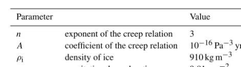
Table 1.Parameters involved in the computation of the vertically averaged horizontal component of the ice velocity (Eq. 4).
Parameter Value
n exponent of the creep relation 3
A coefficient of the creep relation 10−16Pa−3yr−1
ρi density of ice 910 kg m−3
g gravitational acceleration 9.81 m s−2
wherem(t, r)is the surface mass balance andU (t, r)is the vertically averaged horizontal component of the ice veloc-ity in the sheet. In the numerical experiments (see Sects. 4 and 5), we use two different surface mass balances: a func-tion that only depends on the radiusrand a more complex surface mass balance which depends on the atmospheric tem-perature that evolves with the geometry of the ice sheet. Both surface mass balances are described in detail in Appendix A. The velocity of the ice is derived using the shallow ice approximation (Hutter, 1983), which leads to the following analytical formulation of the vertically averaged horizontal component of the ice velocityU (t, r):
U= − 2
n+2A (ρig)
nhn+1
∂s ∂r
n−1
∂s
∂r, (4)
wheres is given by Eq. (1) and the parameters involved in the shallow ice approximation (SIA) are summarised in Ta-ble 1. Since we consider only radially symmetrical ice sheets, a symmetry condition also holds atr=0
U (t,0)=0 and ∂s
∂r(t,0)=0. (5)
2.2 Moving point method
velocity of mesh points is obtained by conserving local mass fractions (Baines et al., 2005, 2011). To calculate the veloc-ity, we first define the total volume of the ice sheetθ (t )as
θ (t )=2π
rl(t ) Z
0
r h(t, r)dr . (6)
Assuming that the flux of ice through the ice sheet margin is zero, its rate of changeθ˙depends only on the surface mass balance,
˙
θ (t )=2π
rl(t ) Z
0
r m(t, r)dr . (7)
We now define the relative mass fractionµ(r)ˆ relative to the moving pointr(t )ˆ . Since the density of iceρiis assumed con-stant, volume fractions and mass fractions are equivalent and
µ(r)ˆ = 2π θ (t )
ˆ r(t ) Z
0
r h(t, r)dr . (8)
The velocity of the moving pointr(t )ˆ is defined implicitly by keepingµ(r)ˆ constant in time, that is,dµ(dtr)ˆ =0. By differen-tiating Eq. (8) with respect to time using the Leibniz integral rule, we obtain the velocity of every interior point
drˆ
dt =U (t,r(t ))ˆ +
1
ˆ
r(t )h(t,r(t ))ˆ
µ(r)ˆ
rl(t ) Z
0
r m(t, r)dr− ˆ r(t ) Z
0
r m(t, r)dr
. (9)
One of the points is dedicated to the static ice divide atr=0, while another point tracks the position of the marginrl(t ),
which moves at the velocity (Bonan et al., 2016) drl
dt =U (t, rl(t ))−m(t, rl(t ))
∂h
∂r
−1
. (10)
Once the velocity of each moving point has been obtained from Eq. (9) or (10), the moving points are moved in a La-grangian manner using the explicit Euler scheme:
ˆ
r(t+1t )= ˆr(t )+1 tdrˆ
dt . (11)
The total mass θ (t )is updated in the same way usingθ (t )˙
from Eq. (7). Finally, the ice thickness profile is updated by differentiating Eq. (8) with respect torˆ, giving
h(t,r(t ))ˆ =θ (t ) π
dµ(r)ˆ
d(rˆ2) . (12)
2.3 Numerical model
From the equations detailed in Sect. 2.2, a finite difference algorithm is derived (see Bonan et al., 2016 for the full al-gorithm). The mesh consists of nr moving nodes with the
positions
0= ˆr1<rˆ2< . . . <rˆnr−1<rˆnr =rl(t ) . (13) No further assumption is made on the spatial distribution of the moving nodes. At each noderˆi there is an associated ice
thicknesshi and a fixed mass fractionµi. By construction,
µ1=0,µnr =1 and the ice thickness at the ice sheet margin
hnr =0 .
The user provides the initial mesh and the ice thickness at mesh points in order to initialise the numerical model. From these quantities, the total mass and the mass fractions at the initial time are calculated by discretising Eqs. (6) and (8) us-ing the followus-ing composite trapezoidal rule:
θ=π
2
nr−1 X
i=1
(hi+hi+1)(rˆi2+1− ˆri2) , (14)
µ1=0, µi+1=µi+
π
2θ(hi+hi+1)(rˆ
2
i+1− ˆri2),
i=1, . . ., nr−1. (15)
The mesh points are then evolved using a discrete form of Eq. (9) and the ice thickness is determined using a discrete form of Eq. (12), with the mass fractions{µi}kept constant
over a time step. Full details are given in Bonan et al. (2016).
3 State estimation of a system modelled with a moving mesh
We now recall the basics of data assimilation before explain-ing how to adapt the 3D-Var and the ETKF methods to our context. We then clarify the form of the observation operator for various types of observations that we assimilate.
3.1 Data assimilation
We consider data assimilation in a discrete dynamical system evolving in time. We denote byxkthe vector of sizenx de-scribing the state of the system at timetk. For example, in our
numerical ice sheet model, ice thicknesses at mesh points are elements of the state vector. The statexk is propagated
for-ward in time to a timetk+1by the non-linear modelMk,k+1. Assuming the model is perfect, we have
xk+1=Mk,k+1(xk) . (16)
Observations are available at timestk and are related toxk
through the equation
whereykis a vector ofpkobservations taken at timetk,Hkis
the (possibly non-linear) observation operator and εk is the
observation error vector, which is assumed to be unbiased (zero mean) with covariance matrixRk.
The objective of DA is to provide an optimal estimatexak
of the system, called the analysis, by combining observations with information derived from the model. We consider in this paper two different DA schemes: a 3D-Var scheme and an ETKF.
3.1.1 3D-Var
The 3D-Var method (see, e.g. Lorenc, 1986; Nichols, 2010) aims to provide the optimal estimate xak by minimising the cost function
J(x)=1
2
x−xbkTBk−1x−xbk +1
2 yk−Hk(x) T
R−k1 yk−Hk(x)
, (18)
wherexbkis a prior, or background, estimate of the state of the system (generally obtained by propagating forward in time the previous analysisxak−1with Eq. 16). The error in the prior estimate is assumed to be unbiased with covariance matrix Bk and to be uncorrelated to errors in the observations.
We take the observation operator Hk to be linear around xb
k, meaning that Hk(x)≈Hk(xbk)+Hk
x−xbk, (19)
where Hk is the linearisation of the observation operator
about the background xbk. Under this assumption, the cost function has an explicit minimum
xak =xbk+Kk
yk−Hk
xbk, (20)
where Kk=BkHTk
HkBkHTk +Rk −1
. (21)
The analysis error covariance matrix can be estimated as
Pe,k=(I−KkHk)Bk. (22)
In theory, the true background error covariance matrixBk
should be updated at each time step. However, this process is extremely expensive for real-time applications and, in-stead, we use a matrix with a simplified structure specified by the user. We will see in the numerical experiments (Sects. 4 and 5) how setting Bk appropriately is essential in order to
obtain good estimates. Although the assimilation scheme we propose here to use with the moving mesh method is a variant of the traditional non-linear 3D-Var method, it is in essence a variational method with a fixed form for the background covariance matrices and we will refer to it as the 3D-Var method in the rest of the paper.
3.1.2 Ensemble transform Kalman filter
The ensemble Kalman filter (EnKF) introduced by Evensen (1994) approximates a fully non-linear Monte Carlo filter. At each time step, the state of the system is represented by an ensemble ofNe realisations
n
x(i)k , i=1, . . ., Ne o
. The state estimate is given by the ensemble mean
xk=
1
Ne Ne X
i=1
x(i)k , (23)
and the state error covariance matrix by the ensemble covari-ance matrix
Pe,k=
1
Ne−1
XkXTk, (24)
whereXkis the anomalies matrix defined as
Xk= h
x(k1)−xk, . . .,x(Nk e)−xk i
. (25)
From the ensemble covariance matrix, we can define the ma-trixCorrthat contains an estimate of the correlation between the state variables to be
[Corr]i,j = [Pe,k]i,j
p
[Pe,k]i,i[Pe,k]j,j
, (26)
where[Corr]i,j and[Pe,k]i,j denote the entry in theith row
andjth column ofCorrandPe,k, respectively.
The forecast step propagates the ensemble from timetk
totk+1with the non-linear modelMk,k+1. For the analysis step, we use the efficient ETKF introduced by Bishop et al. (2001) and follow the implementation of the algorithm given by Hunt et al. (2007).
The ETKF may generate ensembles of analyses with un-derestimated spread, which can lead to the divergence of the filter. We use an inflation procedure (Anderson and Ander-son, 1999) here to avoid this potential degeneracy. In the rest of the paper, the inflation factor is denoted by the parameter
λinfla.
In the twin experiments performed in Sects. 4 and 5, we use a large number of ensembles to avoid producing spuri-ous correlations inPe,k. Therefore, no localisation has been
employed in this paper.
In contrast, the primary characteristic of a moving point method is that the numerical domain evolves in time. The po-sitions of the nodes evolve jointly with the model variables (such as ice thickness) according to the dynamical system equations and can be updated using the assimilation scheme. We therefore include the positions of the nodes in the state vector. As a consequence, we define the state vectorxas fol-lows:
x=
xh xr
withxh=
h1 . . . hnr−1
and xr=
ˆ r2
. . . ˆ rnr
. (27)
Estimates obtained by combining DA with this formulation of x using a moving point numerical model provide more information on the state of the system than if we were using a fixed-grid method.
In particular, for an ice sheet model, this approach gives us a direct estimation of the position of the ice sheet mar-gin that cannot be obtained in fixed-grid methods without interpolation. In this case, we do not include in x the ice thickness at the marginhnr or the position of the ice divide
ˆ
r1 as both are fixed to zero. The DA schemes must, how-ever, provide estimates with strictly positive ice thicknesses
hi,i=1, . . ., nr−1 and a preserved order for node positions
to respect the assumption of the moving mesh scheme. This can be achieved with the 3D-Var method if the spec-ified background covariance matrix Bk in Eq. (21) is
pre-scribed carefully. At timetk, we decompose the background
error covariance matrixBand the tangent linear matrix of the observation operatorH(we drop the time indexkfor clarity) as
B=
Bh BTrh
Brh Br
and H= Hh Hr=
∂H
∂xh
(xf) ∂H ∂xr
(xf)
, (28)
whereBhis the background error covariance matrix between
the model variables,Br is the error covariance between mesh
point locations and Brh includes the cross-covariances
be-tween errors in point locations and errors in model variables. The different components of the state vector are then updated by the following analysis step:
xah=xbh+BhHTh +BTrhHTr HBHT +R −1
y−Hxb (29)
xar =xbr+BrhHTh +BrHTr HBHT+R −1
y−Hxb. (30)
The most difficult step with this form of analysis is, in gen-eral, to set appropriately the cross-covariances in Brh that
are needed for the update stage. For example, if either Hh
orHr is zero, a non-zeroBrhmatrix is the only way to
cor-rect estimates of bothxhandxr. However, we will see in the
next section that in our assimilation systems for the ice sheet model, the observation operator depends explicitly on both ice thickness variables and mesh node locations, and there-fore by settingBrhto zero we can still obtain good estimates.
For the moving point ice sheet model, the DA analysis step updates both ice thickness variables and node positions, but the total mass and mass fractions have to be updated as well, since they are not preserved by the analysis (and there is no reason to preserve them). Therefore, these quantities need to be “reset” from the analysed state vector. This is easily done by using Eqs. (14) and (15). The adapted 3D-Var scheme is performed according to the following steps:
1. calculate a forecast of the state vectorxb by using the
previous analysis solution to initialise the numerical moving point model,
2. use the analysis scheme (Eqs. 29 and 30) to produce the analysisxa,
3. fromxa, calculate the analysed total massθaand update the mass fractionsµausing Eqs. (14) and (15), 4. evolve the analysis solution using the numerical
mov-ing point model to the next time where observations are available and
5. repeat steps 2–5.
The adapted ETKF roughly follows the same path as 3D-Var except that, at step 1, we calculate the forecast for each member of the ensemble and, at step 3, the total mass and mass fractions have to be updated for each member of the en-semble (they are different for each enen-semble member). The background error covariance is also updated using the en-semble statistics. The strict positivity of ice thickness vari-ables and the order required in Eq. (13) for node positions are ensured by appropriately setting the initial ensemble in the ETKF.
We remark that observations outside the domain of the background state at the time of the update cannot be assim-ilated. This is a limitation on both methods, but the ETKF has the advantage that it can take into account such observa-tions if the domain of the background of any member of the ensemble is large enough to include the reference domain. 3.3 Type of observations assimilated
observa-tion operator as
H(x)=
(
hi+ r o− ˆr
i
ˆ
ri+1− ˆri(hi+1−hi) if rˆi≤r o≤ ˆr
i+1
0 elsewhere, (31)
which is merely a piecewise linear interpolation operator. Note thatHdepends on both ice thickness variableshi and
node locationsrˆi. We also assimilate observations of surface
elevation and surface ice velocity. We again use a piecewise linear interpolation operator as in Eq. (31). For observations of surface elevation, we have
H(x)=
(
si+ r o− ˆr
i
ˆ
ri+1− ˆri(si+1−si) if rˆi≤r o≤ ˆr
i+1
b(ri) elsewhere,
(32) with
si =hi+b(ri) . (33)
For observations of surface ice velocity, from a discretisation of Eq. (4) (see Appendix B2 in Bonan et al., 2016), we have
H(x)=
(
us,i+ r o− ˆr
i
ˆ
ri+1− ˆri us,i+1−us,i
ifrˆi≤ro≤ ˆri+1
0 elsewhere,
(34) with
us,i=
1
2A (ρig) 3sgn s
nr −snr−1
h4i
∂b
∂r(ri)
3
+3
5
h5i −h5i−1 ˆ ri− ˆri−1
∂b
∂r(ri)
2
+ 1 3
h3i −h3i−1 ˆ ri− ˆri−1
!2
∂b ∂r(ri)+
27 343
h7i/3−h7i−/31 ˆ
ri− ˆri−1
3 , (35)
except forus,1=0.
We may also assimilate observations of the position of the ice sheet margin. Using a moving point method allows the movement of boundaries to be tracked explicitly. In our con-text, the position of the ice sheet margin is represented by
ˆ
rnr. As a consequence, the observation operator for such an observation is defined by
H(x)= ˆrnr. (36)
The operator is continuous and linear. This makes the assim-ilation of the position of the margin straightforward in com-parison with the same assimilation with a fixed-grid model (see, e.g. Lecavalier et al., 2014).
4 Numerical experiments with an idealised model To demonstrate the efficiency of our DA approach, we per-form twin experiments with two different configurations. In this section, we consider experiments using an idealised sys-tem with a flat bedrock and the EISMINT surface mass bal-ance detailed in Eq. (A1).
Radius (in km)
0 100 200 300 400 500
Altitude (in m)
0 500 1000 1500 2000 2500
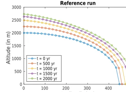
3000 Reference run
t = 0 yr t = 500 yr t = 1000 yr t = 1500 yr t = 2000 yr
Figure 2.Ice thickness profile from the reference run in a simple case (flat bedrock, EISMINT surface mass balance from Eq. A1). The initial state follows the profile of Eq. (37) withh0=2000 m
andrmax=450 km. The reference run is obtained with an initial
mesh ofnr=28 points evenly spaced betweenrˆ1=0 andrˆnr =
450 km.
4.1 Experimental design
We first generate a model run with the moving point numer-ical model from known initial conditions. From this simula-tion, observations are created with added error sampled from a Gaussian distribution. This run is used as a reference to measure the quality of the DA estimates.
We define the reference initial ice thickness profile by the function
h(0, r)=h0 1−
r
rmax 2!3/7
0≤r≤rmax (37)
whereh0=2000 m andrmax=450 km. This function gives a smooth interior profile with a steep snout at the ice sheet marginrmax. This is in compliance with the physics involved in the ice sheet model and provides an initial state with a mar-gin that is immediately in motion. The reference run is ob-tained with an initial mesh ofnr=28 points evenly spaced
betweenrˆ1=0 and rˆnr =450 km. The model time step is
1t=0.02 years, the bed elevationbis fixed to zero and the surface mass balance used is from the EISMINT benchmark (Eq. A1). The experiment starts at timet=0 years and ends att=2000 years. The evolution of the reference ice thick-ness profile can be seen in Fig. 2.
From the reference run, we generate observations of ice thickness and the position of the ice sheet margin at times
t1=500 andt2=1500 years. Observations of thickness are taken at each point except at the margin (a total of 27 ob-servations) with added random noise from the Gaussian dis-tribution N(0, σho2), σho=100 m. For the position of the margin, the observational noise is sampled fromN(0, σro2),
To evaluate the performance of our DA approaches, we compare the estimated ice thickness profiles with their refer-ence counterparts. This is mostly done graphically. We also study the quality of the estimates of two variables: the ice thickness at the ice divide atr=0 and the position of the ice sheet margin.
4.2 Updating the ice thickness only
We begin by studying the performance of the DA schemes in the idealised configuration where we assimilate observations of ice thickness only. We start with an experiment using the 3D-Var algorithm in which only the ice thickness is updated at the assimilation times and the mesh point positions are not updated.
The background state is defined as follows:
– At initial time, the background ice thickness profile is set using the same profile as the reference (Eq. 37) but withh0=2100 m (+5 % error from the reference) and
rmax=472.5 km (also+5 % error).
– The background mesh consists of nr=28 points,
evenly spaced between rˆ1=0 and rˆnr =472.5 km at initial time.
– The model time step is1t=0.02 years.
As we are using a 3D-Var scheme in this experiment, the background error covariance matrixBneeds to be prescribed at both times of assimilation (t1=500 andt2=1500 years). In this first experiment, we only update ice thickness vari-ables, so we set the background error covariance matrix for point positions Br and the cross-covariance matrix Brh to
zero. We define Bh the covariance matrix for ice thickness
variables as
Bh=D1h/2ChD1h/2, (38)
with Dh the diagonal variance matrix and Ch the
correla-tion matrix.Dhis simply set toσhb 2
Inr−1 withσ b
h =100 m.
The background error correlation structure follows a second-order autoregressive (SOAR) distribution with
[Ch]i,j = 1+
| ˆrib− ˆrjb|
Lh !
exp −
| ˆrib− ˆrjb|
Lh !
i, j=1, . . ., nr−1, (39)
where [Ch]i,jdenotes the entry in theith row andjth column
ofCh,rˆibthe location of theith mesh point of the background
state at the time of assimilation and Lh is some correlation
length scale to be fixed. The SOAR function is preferred to a Gaussian structure as the matrixCh is better conditioned
for inversion in that case (Haben et al., 2011). We setLhto
100 km.
This definition of B takes into account the flow depen-dency of the moving point locations, making our approach
adaptive. Figure 3 displaysBhat assimilation timest1=500 and t2=1500 years. As the distance between grid points increases in time in the experiment, the covariances tend to reduce between the two assimilation times. For exam-ple, the covariance between the location of points rˆ1b and
ˆ rnb
r−1 is reduced from[Bh]1,nr−1=530.7 att1=500 years to [Bh]1,nr−1=446.6 at t2=1500 years. In addition, we note decreased correlations for points around the centre of the mesh due to a greater distance between adjacent nodes in the centre of the grid than at the boundaries.
The formulation ofBforces the recomputation of the ma-trix at every assimilation time. This is a limiting factor of our 3D-Var approach, especially for high-dimensional systems, making it cost more than traditional 3D-Var for fixed-grid models in whichBis only computed once. Nevertheless, our experiments demonstrate that this formulation of the back-ground error covariance matrix ensures that the moving point framework produces positive estimates of ice thickness vari-ables and a smooth interior profile in accordance with the physics of the system.
We now evaluate the quality of the estimates. Figure 4 (left) displays the analysed ice thickness profile compared to its background and reference counterparts at the first time of assimilationt1=500 years. The picture shows that the ice thickness profile in the interior of the ice sheet is substan-tially improved by DA. For example, the absolute error in ice thickness at the ice divide (r=0) is reduced from 100 to 58.3 m by the 3D-Var analysis. Results are even better be-tweenr=100 and 400 km. Since we only updatexh in this
experiment, the position of the margin is not modified by our update. Nevertheless, by correcting the interior of the ice sheet, the forecast of the migration of the margin is improved (see the central and right pictures aftert=500 years; Fig. 4), and at the second assimilation time,t=1500 years, the ab-solute difference between the position of the margin before analysis and its reference position is only 5.6 km (instead of 15.9 km without DA).
4.3 Updating ice thickness variables and node positions We now use 3D-Var to update both ice thickness variables and node locations. The definitions ofBhandBrhremain the
same as in the previous experiment, but we set the covariance matrix for node positionsBr to be Br=Dr1/2CrD1r/2 with
Dr the diagonal variance matrix andCr a correlation matrix.
The matrixDr is set toσrb 2
Inr−1withσ b
r =22.5 km andCr
follows a SOAR distribution with [Cr]i,j = 1+
| ˆrib+1− ˆrjb+1| Lr
!
exp −
| ˆrib+1− ˆrjb+1| Lr
!
,
i, j=1, . . ., nr−1, (40)
whereLr is a correlation length scale fixed to 100 km. The
correlation matrixBr constrains the movement of the
[Bh]i,j at time 500 yr
j
5 10 15 20 25
i
5
10
15
20
25
0 2000 4000 6000 8000 10 000
[Bh]i,j at time 1500 yr
j
5 10 15 20 25
i
5
10
15
20
25
0 2000 4000 6000 8000 10 000
Figure 3.Covariance matrices for ice thickness variablesBhused by the 3D-Var at assimilation timest1=500 andt2=1500 years.
Co-variances between variables at distant locations tend to reduce between the two assimilation times. The distance between adjacent nodes also tends to be greater in the centre of the mesh than at the boundaries, leading to a decreasing covariance att2=1500 years in this area.
Radius (in km)
0 100 200 300 400 500
Altitude (in m)
0 500 1000 1500 2000
2500 (a) 3D-Var update, t = 500 yr
Reference No assim 3D-Var Observations
Time (in yr)
0 500 1000 1500 2000
Position margin (in km)
420 440 460 480 500 520
(b) Evolution position margin
Reference No assim 3D-Var
Position grid points (in km) 0 200 400
Time (in yr)
0 500 1000 1500
2000(c) Evolution grid with 3D-Var
Figure 4. (a)3D-Var analysis at timet=500 years compared with the forecast and the reference when we update only ice thickness variables. The ice thickness profile is improved, especially betweenr=100 andr=400 km.(b)Evolution of the position of the margin with time. Even if the position of the margin is not directly updated, the trajectory of the margin is corrected as a result of the ice thickness update.
(c)Evolution of the position of grid points with time. The trajectory of each grid node is corrected after each analysis, as is the margin.
formulation ofBr is selected to ensure that the order of the
points defined by Eq. (13) is preserved by the 3D-Var algo-rithm. Since the distance between nodes evolves in time, it is even more important than in the previous case to use a flow-dependent background error covariance matrixB.
Results for the ice thickness profile are shown in Fig. 5. Overall estimates obtained with updating both ice thickness variables and node positions are better than when we update only ice thickness variables. The absolute error in ice thick-ness at the ice divide (r=0) is reduced from 100 to 60.2 m by the 3D-Var analysis at timet1=500 years, which is sim-ilar to the previous experiment. However, we now obtain at
t1=500 years a very accurate ice thickness profile close to the margin and its estimated position has an absolute error of only 0.2 km. This shows that the estimated position of the ice sheet margin can be accurately corrected by only using standard observations (no observation of the position of the margin is involved in this experiment). At the second time of assimilation att2=1500 years, the estimate is degraded, however, as a result of using fixed variances in the matrixB. This behaviour is discussed further in Sect. 4.5.
The 3D-Var method provides information on the analysis covariance structures for ice thickness variables and mesh point positions. In Fig. 6, we display the estimated standard deviations and the error correlation matrixCorr(see Eq. 26) obtained at timet=500 years using the estimated analysis error covariance matrixPe,k given by Eq. (22). We see that
Radius (in km)
0 100 200 300 400 500
Altitude (in m)
0 500 1000 1500 2000
2500 (a) 3D-Var update, t = 500 yr
Reference No assim 3D-Var Observations
Time (in yr)
0 500 1000 1500 2000
Position margin (in km)
420 440 460 480 500 520
(b) Evolution position margin
Reference No assim 3D-Var
Position grid points (in km) 0 200 400
Time (in yr)
0 500 1000 1500
2000(c) Evolution grid with 3D-Var
Figure 5. (a)3D-Var analysis at timet=500 years compared with the forecast and the reference when we update ice thickness variables and node locations. In contrast to the results shown in Fig. 4, the ice thickness profile is substantially improved close to the margin.(b)Evolution of the position of the margin with time. The estimates are of very good quality even if the margin is not observed directly.(c)Evolution of the position of mesh points with time. The trajectory of each node is corrected by each analysis, as is the margin.
Figure 6.Standard deviations and correlation matrixCorrestimated from the 3D-Var analysis at timet=500 years when we use only observations of ice thickness. Auto-correlations between ice thicknesses are located in the top left corner ofCorr; auto-correlations between node positions are in the bottom right corner. The rest of the matrix depicts the cross-correlations.
4.4 Using an ETKF
We now perform the same experiment as before except that we now use an ETKF. The key question is how to generate the initial ensemble composed ofNe members. The easiest
way is to add noise to a background state sampled from a Gaussian lawN(0,B)withBas the background error covari-ance matrix defined in Eq. (28).
In this experiment, we generate an initial ensemble of
Ne=200 members using:
– the same background state used in the experiments de-tailed in Sect. 4.2 and 4.3,
– Bh defined by Eq. (38) with the diagonal matrixDh=
σh2Inr−1, σ b
h =100 m, Ch defined by Eq. (39), Lh=
100 km,
– Br taken as D1r/2CrD1r/2 withCr defined by Eq. (40)
withLh=100 km and the diagonal matrixDr defined
as
[Dr]ii=min
σrb, αrˆi
i=1, . . ., nr−1 (41)
withσrb=22.5 km andα=0.2, and – Brhset to zero.
Note that the definition of Bis slightly different from the previous experiment as we choose different diagonal vari-ances. The change is because of the high probability of generating useless initial meshes with negative radii using Dr =σrb
2
Inr−1, as the background standard deviationσ b r is
Radius (in km)
0 100 200 300 400 500
Altitude (in m)
0 500 1000 1500 2000
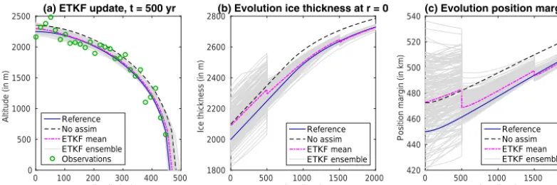
2500 (a) ETKF update, t = 500 yr
Reference No assim ETKF mean ETKF ensemble Observations
Time (in yr)
0 500 1000 1500 2000
Ice thickness (in m)
1800 2000 2200 2400 2600
2800(b) Evolution ice thickness at r = 0
Reference No assim ETKF mean ETKF ensemble
Time (in yr)
0 500 1000 1500 2000
Position margin (in km)
420 440 460 480 500 520
540(c) Evolution position margin
Reference No assim ETKF mean ETKF ensemble
Figure 7. (a)ETKF analysis at timet=500 years compared with the forecast and the reference. The ice thickness profile is improved over the whole domain and the reference profile is within the ensemble spread.(b)Evolution of the ice thickness atr=0 with time. The estimates are of very good quality and the estimates seem to converge towards the reference value at the end of the study.(c)Evolution of the position of the margin with time. The ETKF provides consistent estimates and the reference value is always within the ensemble spread.
Est. [corr] at t = 500 yri,j
Index j
10 20 30 40 50
Index i
10
20
30
40
50
-1 -0.5 0 0.5 1
Radius (in km)
0 100 200 300 400 500
SD h (blue x, in m)
0 20 40 60 80 100
Est. standard deviations at 500 yr
SD r (orange +, in km)
0 5 10 15 20 25
Figure 8.Standard deviations and correlation matrixCorrestimated from the ETKF analysis ensemble at timet=500 years when we use only observations of ice thickness. Auto-correlations between ice thicknesses are located in the top left corner ofCorr; auto-correlations between node positions are in the bottom right corner. The rest of the matrix depicts the cross-correlations.
of 472.9 km with an estimated standard deviation of 22.8 km (where the true value att=0 is 450 km).
We do not use any inflation in this experiment (λinfla=1). Results are summarised in Fig. 7. At the first time of as-similationt1=500 years, the analysis step corrects the ice thickness profile well. The estimate of the ice thickness at
r=0 is of the same quality as in the previous experiments (absolute error of 46.9 m) and the estimate of the position of the margin is reduced from 483.1 km (forecast mean with estimated standard deviation 18.9 km) to 468.8 km (analysis mean with estimated standard deviation 7.1 km). The esti-mate obtained by the ETKF is in accordance with the true value (which is within the ensemble spread) and the absolute error of 7.5 km is of the same order as the estimated stan-dard deviation. The rest of the experiment exhibits the same quality in terms of recovering the ice thickness profile.
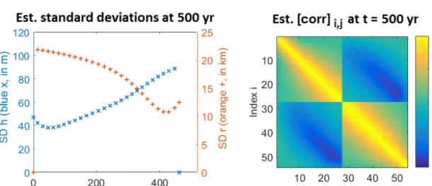
The ETKF provides information on the covariance struc-tures for ice thickness variables and mesh point positions. We display estimated standard deviations and an estimate of the correlation matrixCorr(see Eq. 26) in Fig. 8 for the analy-sis ensemble at timet=500 years. The ETKF produces
de-creased standard deviations and correlation length scales for ice thickness variables close to the ice divide. For example, the standard deviation of the ice thickness at the ice divide is more than halved by the analysis, from 97.4 m before analy-sis to 41.6 m. Decreased standard deviations and correlation length scales are also obtained for node locations but close to the margin in this case. The standard deviation for the posi-tion of the margin is reduced from 18.9 km to 7.1 km by the analysis. The ETKF also produces strong anti-correlations between ice thickness variables and node positions, meaning that where ice thickness variables become larger associated nodes need to retreat to fit the observations of ice thickness. 4.5 Comparing 3D-Var and the ETKF
We now compare the results from applying the 3D-Var and ETKF assimilation schemes in the case where we observe only the ice thickness. We focus on the accuracy of the esti-mated ice thickness atr=0 and the position of the margin.
Time (in yr)
0 500 1000 1500 2000
(in m)
0 10 20 30 40 50 60 70 80 90 100
Absolute error ice thickness r = 0
No assim 3D-Var no grid update 3D-Var grid update ETKF mean
Time (in yr)
0 500 1000 1500 2000
(in km)
0 5 10 15 20
25Absolute error position of the margin No assim
3D-Var no grid update 3D-Var grid update ETKF mean
Figure 9.Evolution of the absolute error of the estimated ice thickness atr=0 and the estimated position of the margin when we observe only the ice thickness. We compare the absolute errors obtained when we use 3D-Var without and with correction of the position of grid nodes and when we use an ETKF.
Figure 10.The background error covariance matrices used by the 3D-Var and ETKF methods to produce the analysis at timet=1500 years.
node updates. All three methods provide improved estimates at the first analysis time (t1=500 years), leading to good forecasts up to the next assimilation time. We find that the ETKF tends to perform better than the variational approach and that for 3D-Var the estimates obtained by updating both ice thickness variables and node positions are generally bet-ter than those where only ice thickness variables are updated. For 3D-Var without node updates, the analysis at the sec-ond time of assimilation (t2=1500 years) of the ice thick-ness at r=0 is unfortunately degraded relative to the fore-cast, but the estimated position of the margin is still im-proved by the second analysis. In the case where ice ness and nodes are updated, the estimates of both ice thick-ness atr=0 and the position of the margin are degraded at the second time of assimilation. This weakens the confidence in the forecast and we partially lose what we had gained from the previous analysis. The experiment shows the sensitivity of 3D-Var to current observations resulting from the depen-dence of the prescribed covariance matrixBon the positions of the mesh nodes.
Using the ETKF assimilation scheme, where the covari-ance matrix fully evolves in time, is seen to improve the overall estimates. At each assimilation time, the errors in the estimated ice thickness and the position of the margin are de-creased. Notably, we do not observe any degrading of the es-timates at the second time of assimilation. This improvement can be attributed to the better background forecast produced by the ETKF at each assimilation time.
Time (in yr)
0 500 1000 1500 2000
(in m)
0 10 20 30 40 50 60 70 80 90 100
Absolute error ice thickness r = 0
No assim 3D-Var grid update ETKF mean
Time (in yr)
0 500 1000 1500 2000
(in km)
0 5 10 15 20
25 Absolute error position of the margin No assim
3D-Var grid update ETKF mean
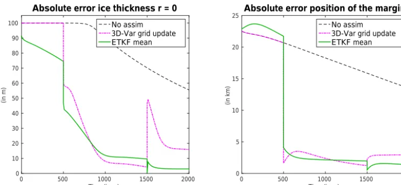
Figure 11.Evolution of the absolute error of the estimated ice thickness atr=0 and the estimated position of the margin when we observe the ice thickness and the position of the margin. We compare the absolute errors obtained when we use 3D-Var with correction of the position of grid nodes and when we use an ETKF. In both experiments, the results are improved with respect to the position of the margin (compared to results detailed in Fig. 9). No improvement (nor degradation) is observed for the ice thickness atr=0.
Propagating the background error covariances using the en-semble statistics ensures that the ETKF is a more reliable scheme than 3D-Var. This improvement has a computational cost, however, as we now need to run the model Ne times
instead of once for 3D-Var.
4.6 Assimilating observations of the position of the margin
In this section, we perform the same experiments as previ-ously, but we now assimilate not only the same observations of ice thickness as before but also observations of the posi-tion of the margin. We consider only the case of 3D-Var with grid update and the ETKF.
Absolute errors for the estimates of the ice thickness at
r=0 and the position of the margin are shown in Fig. 11. In both cases, assimilating observations of the position of the margin is beneficial to our estimates of the margin and of the ice thickness profile close to the margin. For example, the estimated position of the margin at timet=500 years has an absolute error of 4.2 km for the ETKF (compared to 7.5 km previously). Not surprisingly, it does not change the results for the ice thickness atr=0.
Adding observations of the position of the margin in the data assimilation system reduces the estimated standard de-viations obtained with the ETKF for variables close to the margin. For example, the estimated standard deviation for the position of the margin is now 5.8 km instead of 7.1 km. Not surprisingly it has no influence on the standard deviation for variables close to the ice divide. The estimated correlation structure (not shown) is also not modified by adding obser-vations of the position of the margin in the DA system.
5 Numerical experiments with an advanced configuration
In this section, we consider experiments using a more real-istic configuration with a non-flat bedrock and an advanced surface mass balance, detailed in Appendix A2. We inves-tigate the case of a rapidly warming climate over a short timescale.
5.1 Experimental Design
We generate observations from a new reference run. We use a non-flat fixed bedrock whose elevation is defined by the equation
b(r)=1000 m−1400 m· r
1000 km 2
+700 m· r
1000 km 4
−120 m· r
1000 km 6
. (42) The reference run is generated from a realistic initial state obtained with the following steps:
– Start with an ice sheet profile following Eq. (37) withh0=2000 m,rmax=300 km andnr=21
compu-tational mesh points evenly spaced betweenrˆ1=0 and
ˆ
rnr =300 km.
– Run the numerical model with a fixed climate forc-ing, as defined in Eq. (A4), where Tclim=4◦C until it reaches the steady state (a 30 000-year run with a
1t=0.01-year time step).
Radius (in km)
0 200 400 600 800 1000 1200
Altitude (in m)
0 1000 2000 3000 4000
5000 Reference initial state Bed elevation Surface elevation
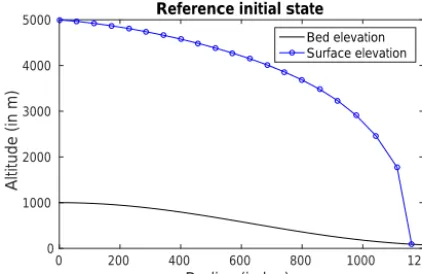
Figure 12.Initial state used to obtain a 20-year reference run under a warming climate as detailed in Sect. 5.1 withnr=21 grid points and a non-flat bed.
0.01 years). The state obtained at the end of the run is the initial state (see Fig. 12).
The reference is obtained by running the model over 20 years from the initial state with a time step 1 t=
0.01 years and the same linearly warming climate forc-ing as defined in Appendix A.2, with Tclim=6◦C at initial timet=0 years, andTclim=6.4◦C att=20 years (that is,
Tclim=6+0.2t). Over the 20-year run, the geometry of the ice sheet stays relatively similar to the geometry of the initial state due to the slow dynamics of the model. The ice sheet margin retreats from 1160.9 to 1158.6 km and the ice thick-ness at the ice divide increases by 1.5 m.
We generate observations of surface elevation, surface ice velocity and the position of the ice sheet margin at timest=
1,2, . . .,10 years from the reference run. The observations of the surface are taken at each point including the margin with an added Gaussian noise (uncorrelated with standard deviation σso=200 m). The observations of the surface ice velocity are located at the midpoints between mesh points (so we have 20 observations of surface velocity). Observations are noised using a Gaussian law (standard deviation σuo
s = 30 m yr−1, uncorrelated). For the position of the margin, the observational noise is sampled from N(0, σro2)withσro=
50 km.
We compare the influence of the observations on the qual-ity of the DA estimates and the subsequent forecasts for the 3D-Var and ETKF methods. Again, we focus on the two vari-ables: the ice thickness at the ice divide atr=0 and the po-sition of the ice sheet margin.
5.2 Assimilating observations of surface elevation We begin by studying the performance of the DA schemes where we assimilate only observations of surface elevations. For 3D-Var, the estimates are obtained using an initial background state defined as xb=0.95xref(0) with a 5 % smaller extent than the reference state. The flow-dependent
background error covariance matrix B is defined as in Eq. (28). The matrixBhis defined as in Eq. (38) with a SOAR
matrix forCh(σhb=200 m,Lh=240 km) andBr is defined
with a SOAR matrix forCr(σrb=60 km,Lr=240 km). The
matrixBrhis set to0.
The ETKF uses an ensemble with 200 members. The ini-tial ensemble is generated by adding toxb a random noise
drawn from the Gaussian lawN(0,B). The background co-variance matrixBis defined as previously, except forBr for
which we still use a SOAR matrix for Cr (Lr =240 km)
but with variances decreased near the ice divide following Eq. (41) (σrb=60 km andα=0.2). We tested different val-ues for the inflation parameterλinfla; the best results were obtained withλinfla=1.01.
We first study the results obtained with the ETKF. At the end of the data assimilation window,t=10 years, the ice thickness profile is retrieved well everywhere by the mean of the ensemble and the reference profile is within the ensem-ble spread (see Fig. 13). We note that the estimate of the ice thickness at the ice divide is improved by the first analysis. After timet=7 years, however, the estimate is worsened by the analysis. This is because the ensemble spread is too small from that time onwards. This can be fixed by taking a larger inflation parameterλinfla, but the estimates of other variables are then degraded. The estimated position (mean) of the mar-gin att=10 years is 1158.0 km with an ensemble standard deviation of 3.1 km. In comparison to the reference value at that time,r=1159.9 km, we see that the ETKF with a large ensemble performs well. The quality of the estimates is also kept high during the forecast (fromt=10 tot=20 years). For example, the absolute error on the position of the margin is kept below 2.5 km over this time window.
With respect to the covariance matrix, the estimates seem to show a similar behaviour to those of the experiment de-tailed in Sect. 4.4 using the ETKF where observations of ice thickness are assimilated (see Fig. 14), but with a larger correlation length scale. The similarity can be explained by the similarity of the construction of the initial ensemble (the same structure for the background covariance matrixBused to sample the Gaussian noise added to the background state) and by the similarity of the observation operators for ice thickness and surface elevation.
Radius (in km) 0 500 1000
Altitude (in m)
0 1000 2000 3000 4000 5000
(a) Ice sheet geometry, t = 10 yr
Bed elevation Reference No assim ETKF mean ETKF ensemble
Time (in yr)
0 5 10 15 20
Ice thickness (in m)
3400 3600 3800 4000 4200
4400(b) Evolution ice thickness at r = 0
Reference No assim ETKF mean ETKF ensemble
Time (in yr)
0 5 10 15 20
Position margin (in km)
1000 1050 1100 1150 1200 1250
1300(c) Evolution position margin
Reference No assim ETKF mean ETKF ensemble
Figure 13.ETKF results for the advanced configuration where observations of surface elevation are assimilated over the first 10 years and a forecast is made for 10 further years.(a)ETKF analysis at timet=10 years compared with the reference.(b)Evolution of the ice thickness atr=0 with time.(c)Evolution of the position of the margin with time.
Est. [corr]i,j at t = 10 yr
Index j
10 20 30 40
Index i
10
20
30
40 -1
-0.5 0 0.5 1
Radius (in km)
0 500 1000
SD h (blue x, in m)
0 50 100
Est. standard deviations at 10 yr
SD r (orange +, in km)
0 50
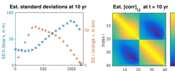
Figure 14. Standard deviations and correlation matrixCorr estimated from the analysis ensemble at timet=10 years in the advanced configuration where we observe surface elevation. The matrixCorrhas the same structure asBdefined by Eq. (28). Both standard deviations and correlation structures are similar to Fig. 8.
3D-Var does not assimilate all available data. Indeed, the algorithm cannot incorporate observations outside the back-ground domain because of the form of the observation opera-tor (see Eq. 32). This is not, however, the case for the ETKF, even if the ensemble mean has a smaller domain than the ref-erence domain, since in this case there is at least one member of the ensemble with a bigger domain than that of the refer-ence. At the end, both approaches show a similar accuracy in the forecast state after timet=10 years, showing again the efficiency of both DA schemes.
5.3 Assimilating observations of surface velocity and position of the margin
We now consider assimilating observations of surface ice ve-locity and the position of the margin (if we only assimilate observations of surface ice velocity, the problem is undeter-mined).
Again, we want to compare the accuracy of 3D-Var and the ETKF using this new set of observations. We use the same background state, the same structure forBand the same
ini-tial ensemble as before. The observation operator for surface velocities is non-linear (see Eq. 35) and, even though the en-semble is large, inflation is necessary in this case. We take an inflation ofλinfla=1.10. If the inflation is taken any larger in this example, the ETKF analysis produces ensemble mem-bers with a non-ordered grid and the experiment cannot be pursued.
We first study the results obtained with the ETKF. At the end of the DA window,t=10 years, the ice thickness profile is retrieved well everywhere by the mean of the ensemble, except near the ice divide atr=0 (see Fig. 16). This is due to the relatively large uncertainty of surface velocity obser-vations near the ice divide compared to the reference value at the same point (hereσuo
s=30 m yr
Time (in yr)
0 5 10 15 20
(in m)
0 50 100 150 200
250 Absolute error ice thickness r = 0
No assim 3D-Var grid update ETKF mean
Time (in yr)
0 5 10 15 20
(in km)
0 10 20 30 40 50 60
Absolute error position of the margin
No assim 3D-Var grid update ETKF mean
Figure 15.Evolution of the absolute error of the estimated ice thickness atr=0 and the estimated position of the margin in the advanced configuration where we assimilate surface elevations over the first 10 years. We compare the absolute errors obtained when we use 3D-Var with the correction of the position of grid nodes and when we use an ETKF. The ETKF performs better than the 3D-Var for both variables.
Radius (in km) 0 500 1000
Altitude (in m)
0 1000 2000 3000 4000 5000
(a) Ice sheet geometry, t = 10 yr
Bed elevation Reference No assim ETKF mean ETKF ensemble
Time (in yr)
0 5 10 15 20
Ice thickness (in m)
3400 3600 3800 4000 4200
4400(b) Evolution ice thickness at r = 0
Reference No assim ETKF mean ETKF ensemble
Time (in yr)
0 5 10 15 20
Position margin (in km)
1000 1050 1100 1150 1200 1250
1300 (c) Evolution position margin
Reference No assim ETKF mean ETKF ensemble
Figure 16. ETKF results for the advanced configuration where observations of surface ice velocity and the position of the margin are assimilated over the first 10 years and a forecast is made for the following 10 years.(a)ETKF analysis at timet=10 years compared with the reference.(b)Evolution of the ice thickness atr=0 with time.(c)Evolution of the position of the margin with time.
the forecasts obtained after t=10 years since estimates of the position of the margin are not degraded over the time window[10, 20 years].
Estimates of the standard deviations and covariances, as shown in Fig. 17, differ from those of the previous experi-ment (see Fig. 14 for comparison). The reduction in the stan-dard deviation for ice thickness variables close to the ice di-vide is less significant than in the previous experiment. This is due to the relatively large uncertainty of surface veloc-ity observations near the ice divide compared to the refer-ence value at the same point. We remark that assimilating observations of surface ice velocity together with the posi-tion of the margin leads to an increased correlaposi-tion length scale for ice thickness variables and to a smaller correla-tion length scale for node posicorrela-tions compared to the previ-ous experiment. Finally, the cross-covariances have smaller anti-correlations and positive correlations appear between ice thickness variables in the interior of the ice sheet and be-tween node positions close to the margin. These differ sig-nificantly from the case where we assimilate observations of
surface elevation as a result of the difference in observation operators.
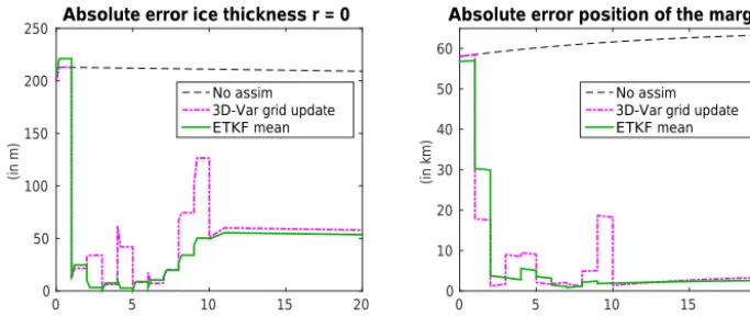
We finally compare the ETKF with results obtained with 3D-Var. Absolute errors in the ice thickness atr=0 and in the position of the margins are displayed for both cases in Fig. 18. As in previous experiments, the ETKF performs bet-ter than 3D-Var for the position of the margin, but 3D-Var gives better results for the ice thickness atr=0 and performs reasonably well overall in this non-linear context. The fore-cast trajectory of the margin aftert=10 is improved by DA in both cases. This demonstrates again the robustness of our DA approach in the context of an ice sheet modelled with a moving point numerical model.
6 Conclusion and prospects
Est. [corr]i,j at t = 10 yr
Index j
10 20 30 40
Index i
10
20
30
40 -1
-0.5 0 0.5 1
Radius (in km)
0 500 1000
SD h (blue x, in m)
0 50 100
Est. standard deviations at 10 yr
SD r (orange +, in km)
0 50
Figure 17. Standard deviations and correlation matrixCorr estimated from the analysis ensemble at timet=10 years in the advanced configuration where we observe surface ice velocity and the position of the margin. The matrixCorrhas the same structure asBdefined by Eq. (28). Both standard deviations and cross-correlation structures are different from those shown in Fig. 14.
Time (in yr)
0 5 10 15 20
(in m)
0 50 100 150 200
250 Absolute error ice thickness r = 0
No assim 3D-Var grid update ETKF mean
Time (in yr)
0 5 10 15 20
(in km)
0 10 20 30 40 50 60
Absolute error position of the margin
No assim 3D-Var grid update ETKF mean
Figure 18.Evolution of the absolute error of the estimated ice thickness atr=0 and the estimated position of the margin when we observe surface ice velocities and the position of the margin in the advanced configuration. We compare the absolute errors obtained when we use 3D-Var with the correction of the grid-node positions and when we use an ETKF. The ETKF performs better than the 3D-Var with respect to the position of the margin, but 3D-Var gives better results for the ice thickness atr=0 in this case.
the location of mesh nodes in the state vector. The only re-quirement is to ensure that the update does not produce a non-ordered moving mesh. This can be achieved empirically either by using an appropriate flow-dependent background covariance matrix with large correlations between adjacent mesh points or by using an ensemble with the same proper-ties. This combination has been validated with various twin experiments assimilating classical available observations for an ice sheet (ice thickness, surface elevation and surface ice velocity) and also observations of the position of the bound-ary. These twin experiments show the following:
– The form of the state vector allows the explicit tracking of boundary positions for moving boundary problems.
– This form also allows a straightforward and efficient as-similation of boundary positions (in this paper, the po-sition of the margin).
– Assimilating spatially distributed observations gives better estimates if node locations are updated in the analysis step.
– 3D-Var can have issues with assimilating observations if they are located outside the forecast domain; the ETKF can overcome these issues if at least one member of the ensemble has its numerical domain large enough to in-clude the location of these observations.
– ETKF tends to provide better estimates than 3D-Var, mainly because of its capacity to provide flow-dependent statistical estimates of the background error covariances, but 3D-Var still provides satisfactory esti-mates.
Whilst this paper uses a particular moving mesh method for the 1-D numerical model, our approach can be extended to any 1-D moving boundary problem modelled with a moving mesh, assuming only that the ordering of the points must be maintained.
Moving mesh approaches are also suitable for modelling the evolution of 2-D moving boundary phenomena (Baines et al., 2009). The successful application of the moving mesh method to a 2-D model of an ice cap is presented in Partridge (2013). Initial results on the assimilation of observations of ice thickness into the 2-D ice cap model are also given in Par-tridge (2013). These results raise a number of issues concern-ing the approach needed for updatconcern-ing the nodal positions of the 2-D grid during the assimilation step. Research on these issues is ongoing.
Appendix A: Surface mass balances A1 EISMINT surface mass balance
For the twin experiments performed in Sect. 4, we use the simple constant-in-time surface mass balance employed in the moving margin experiments of the EISMINT intercom-parison project (Huybrechts et al., 1996):
m(r)=min0.5 m yr−1,10−2m yr−1km−1·(450 km−r). (A1) A2 Parameterised surface mass balance with feedback
loop
For the twin experiments performed in Sect. 5, we use a more complex surface mass balance parameterised as a function of the surface atmospheric temperatureTs(t, r). This simple
pa-rameterisation was used in Bonan et al. (2014) in the context of ice sheet model initialisation but with a fixed-grid model. The values of the different parameters involved in this pa-rameterisation are given in Table A1. The surface mass bal-ance is the sum of positive accumulation Acc (snow precipi-tation) and negative ablation Abl (melting) parameterised in Eqs. (A2) and (A3).
Acc(t, r)=Acc0ec0Ts (A2)
Abl(t, r)=
Abl0
T s−T0
T0 2
ifTs> T0
0 otherwise
(A3)
The surface temperature depends on the altitude of the sur-faces, the distance from the origin and a climate temperature
Tclim(t )evolving in time according the relation
Ts(t, r)=Tclim(t )+λ r+γ s(t, r). (A4)
This parameterisation aims to reproduce qualitatively a typ-ical surface mass balance over an ice sheet and to include feedbacks associated with the evolution of the geometry. Table A1.List of parameter values used for the parameterised sur-face mass balance.
Parameter Value
Acc0 rate of accumulation 6 m yr−1
Abl0 rate of ablation −5 m yr−1
T0 minimum temperature for −6◦C
ablation
c0 coefficient exponential law 0.115◦C−1
for accumulation
λ longitudinal gradient of 111 0001 ◦C m−1 surface temperature
Competing interests. The authors declare that they have no conflict of interest.
Acknowledgements. This research was funded in part by the Natural Environmental Research Council National Centre for Earth Observation (NCEO) and the European Space Agency (ESA).
Edited by: Olivier Talagrand
Reviewed by: two anonymous referees
References
Anderson, J. L. and Anderson, S. L.: A Monte Carlo im-plementation of the nonlinear filtering problem to pro-duce ensemble assimilations and forecasts, Mon. Weather Rev., 127, 2741–2758, https://doi.org/10.1175/1520-0493(1999)127<2741:AMCIOT>2.0.CO;2, 1999.
Baines, M. J., Hubbard, M. E., and Jimack, P. K.: A mov-ing mesh finite element algorithm for the adaptive solu-tion of time-dependent partial differential equasolu-tions with moving boundaries, Appl. Numer. Math., 54, 450–469, https://doi.org/10.1016/j.apnum.2004.09.013, 2005.
Baines, M. J., Hubbard, M. E., Jimack, P. K., and Mahmood, R.: A moving-mesh finite element method and its application to the nu-merical solution of phase-change problems, Commun. Comput. Phys., 6, 595–624, 2009.
Baines, M. J., Hubbard, M. E., and Jimack, P. K.: Velocity-based moving mesh methods for nonlinear partial differ-ential equations, Commun. Comput. Phys., 10, 509–576, https://doi.org/10.4208/cicp.201010.040511a, 2011.
Berger, M. J. and Oliger, J.: Adaptive mesh refinement for hyper-bolic partial differential equations, J. Comput. Physics, 53, 484– 512, 1984.
Bishop, C. H., Etherton, B. J., and Majumdar, S. J.: Adap-tive sampling with the Ensemble Transform Kalman Filter. Part I: Theoretical aspects, Mon. Weather Rev., 129, 420–436, https://doi.org/10.1175/1520-0493(2001)129<0420:ASWTET>2.0.CO;2, 2001.
Blayo, E., Bocquet, M., Cosme, E., and Cugliandolo, L. F.: Ad-vanced Data Assimilation for Geosciences, Lecture Notes of the Les Houches School of Physics: Special Issue, June 2012, Ox-ford University Press, OxOx-ford, UK, 2014.
Bonan, B., Nodet, M., Ritz, C., and Peyaud, V.: An ETKF approach for initial state and parameter estimation in ice sheet modelling, Nonlin. Processes Geophys., 21, 569–582, https://doi.org/10.5194/npg-21-569-2014, 2014.
Bonan, B., Baines, M. J., Nichols, N. K., and Partridge, D.: A moving-point approach to model shallow ice sheets: a study case with radially symmetrical ice sheets, The Cryosphere, 10, 1–14, https://doi.org/10.5194/tc-10-1-2016, 2016.
Budd, C. J., Huang, W., and Russell, R. D.: Adaptiv-ity with moving grids, Acta Numerica, 18, 111–241, https://doi.org/10.1017/S0962492906400015, 2009.
Cao, W., Huang, W., and Russell, R. D.: Approaches for gener-ating moving adaptive meshes: location versus velocity, Appl. Numer. Math., 47, 121–138, https://doi.org/10.1016/S0168-9274(03)00061-8, 2003.
Church, J. A., Clark, P. U., Cazenave, A., Gregory, J. M., Jevrejeva, S., Leverman, A., Merrifield, M. A., Milne, G. A., Nerem, R. S., Nunn, P. D., Payne, A. J., Pfeffer, W. T., Stammer, D., and Un-nikrishnan, A. S.: Sea level change, in: Climate Change 2013: The Physical Science Basis, Contribution of Working Group I to the Fifth Assessment Report of the Intergovernmental Panel on Climate Change, edited by: Stocker, T. F., Qin, D., Plattner, G.-K., Tignor, M., Allen, S. K., Boschung, J., Nauels, A., Xia, Y., Bex, V., and Midgley, P. M., , Cambridge University Press, Cambridge, UK, New York, NY, USA, 1137–1216, 2013. Cornford, S. L., Martin, D. F., Graves, D. T., Ranken, D. F.,
Le Brocq, A. M., Gladstone, R. M., Payne, A. J., Ng, E. G., and Lipscomb, W. H.: Adaptive mesh, finite volume model-ing of marine ice sheets, J. Comput. Physics, 232, 529–549, https://doi.org/10.1016/j.jcp.2012.08.037, 2013.
Cornford, S. L., Martin, D. F., Lee, V., Payne, A., and Ng, E. G.: Adaptive mesh refinement versus subgrid friction interpolation in simulations of Antarctic ice dynamics, Ann. Glaciol., 57, 1–9, https://doi.org/10.1017/aog.2016.13, 2016.
Dyke, A. S. and Prest, V. K.: Late Wisconsinan and Holocene Re-treat of the Laurentide Ice Sheet. Scale 1:5 000 000, Map 1702A, Geological Survey of Canada, Ottawa, Ontario, Canada, 1987. Evensen, G.: Sequential data assimilation with a nonlinear
quasi-geostrophic model using Monte Carlo methods to forecast error statistics, J. Geophys. Res.-Oceans, 99, 10143–10162, https://doi.org/10.1029/94JC00572, 1994.
Gladstone, V., Lee, A., Vieli, A., and Payne, A. J.: Grounding line migration in an adaptive mesh ice sheet model, J. Geophys. Res.-Earth, 115, F04014, https://doi.org/10.1029/2009JF001615, 2010.
Haben, S. A., Lawless, A. S., and Nichols, N. K.: Conditioning of incremental variational data assimilation, with application to the Met Office system, Tellus A, 63, 782–792, 2011.
Hunt, B. R., Kostelich, E. J., and Szunyogh, I.: Efficient data assimilation for spatiotemporal chaos: A local en-semble transform Kalman filter, Physica D, 230, 112–126, https://doi.org/10.1016/j.physd.2006.11.008, 2007.
Hutter, K.: Theoretical Glaciology, D. Reidel, Dordrecht, the Netherlands, 1983.
Huybrechts, P., Payne, A. J., and The EISMINT Intercomparison Group: The EISMINT benchmarks for testing ice-sheet models, Ann. Glaciol., 23, 1–12, 1996.
Lahoz, W., Khattatov, B., and Menard, R. E.: Data assimilation: making sense of observations, Springer-Verlag, Berlin, Germany, https://doi.org/10.1007/978-3-540-74703-1, 2010.
Lecavalier, B. S., Milne, G. A., Simpson, M. J. R., Wake, L., Huy-brechts, P., Tarasov, L., Kjeldsen, K. K., Funder, S., Long, A. J., Woodroffe, S., Dyke, A. S., and Larsen, N. K.: A model of Greenland ice sheet deglaciation constrained by observations of relative sea level and ice extent, Quaternary Sci. Rev., 102, 54– 84, https://doi.org/10.1016/j.quascirev.2014.07.018, 2014. Lee, T. E., Baines, M. J., Langdon, S., and Tindall,
M. J.: A moving mesh approach for modelling avas-cular tumour growth, Appl. Numer. Math., 72, 99–114, https://doi.org/10.1016/j.apnum.2013.06.001, 2013.
Li, Y., Jeong, D., and Kim, J.: Adaptive mesh refinement for simulation of thin film flows, Meccanica, 49, 239–252, https://doi.org/10.1007/s11012-013-9788-6, 2014.
Lorenc, A. C.: Analysis methods for numerical weather prediction, Q. J. Roy. Meteor. Soc., 112, 1177–1194, https://doi.org/10.1002/qj.49711247414, 1986.
Lukyanov, A. V., Sushchikh, M. M., Baines, M. J., and Theo-fanous, T. G.: Superfast nonlinear diffusion: Capillary trans-port in particulate porous media, Phys. Rev. Lett., 109, 214501, https://doi.org/10.1103/PhysRevLett.109.214501, 2012. Mathiot, P., König Beatty, C., Fichefet, T., Goosse, H., Massonnet,
F., and Vancoppenolle, M.: Better constraints on the sea-ice state using global sea-ice data assimilation, Geosci. Model Dev., 5, 1501–1515, https://doi.org/10.5194/gmd-5-1501-2012, 2012. Nichols, N. K.: Mathematical concepts of data assimilation, in: Data
assimilation: making sense of observations, edited by: Lahoz, W., Khattatov, B. and Menard, R., Springer-Verlag, Berlin, Germany, 13–40, 2010.
Partridge, D.: Numerical modelling of glaciers: moving meshes and data assimilation, PhD thesis, University of Reading, Read-ing, Berks, United Kingdom, available at: http://www.reading. ac.uk/web/FILES/maths/DP_PhDThesis.pdf (last access: 28 Au-gust 2017), 2013.
Sarahs, N.: Similarity, Mass Conservation, and the Nu-merical Simulation of a Simplified Glacier Equation, SIAM Undergraduate Research Online, 9, S014019, https://doi.org/10.1137/15S014198, 2016.