www.nonlin-processes-geophys.net/13/601/2006/ © Author(s) 2006. This work is licensed
under a Creative Commons License.
Nonlinear Processes
in Geophysics
Synchronicity in predictive modelling: a new view of data
assimilation
G. S. Duane1, J. J. Tribbia1, and J. B. Weiss2
1National Center for Atmospheric Research, PO Box 3000, Boulder, CO 80307, USA
2Department of Atmospheric and Oceanic Sciences, UCB 311, University of Colorado, Boulder, CO 80309, USA Received: 16 March 2006 – Revised: 15 August 2006 – Accepted: 5 September 2006 – Published: 3 November 2006
Abstract. The problem of data assimilation can be viewed as one of synchronizing two dynamical systems, one repre-senting “truth” and the other reprerepre-senting “model”, with a unidirectional flow of information between the two. Syn-chronization of truth and model defines a general view of data assimilation, as machine perception, that is reminiscent of the Jung-Pauli notion of synchronicity between matter and mind. The dynamical systems paradigm of the synchroniza-tion of a pair of loosely coupled chaotic systems is expected to be useful because quasi-2D geophysical fluid models have been shown to synchronize when only medium-scale modes are coupled. The synchronization approach is equivalent to standard approaches based on least-squares optimization, in-cluding Kalman filtering, except in highly non-linear regions of state space where observational noise links regimes with qualitatively different dynamics. The synchronization ap-proach is used to calculate covariance inflation factors from parameters describing the bimodality of a one-dimensional system. The factors agree in overall magnitude with those used in operational practice on an ad hoc basis. The calcu-lation is robust against the introduction of stochastic model error arising from unresolved scales.
1 Introduction
A computational model of a physical process that provides a stream of new data to the model as it runs must include a scheme to combine the new data with the model’s predic-tion of the current state of the process. The goal of any such scheme is the optimal prediction of the future behavior of the physical process. While the relevance of the data assimila-tion problem is thus quite broad, techniques have been in-vestigated most extensively for weather modeling, because Correspondence to: G. S. Duane
of the high dimensionality of the fluid dynamical state space, and the frequency of potentially useful new observational in-put. Existing data assimilation techniques (3DVar, 4DVar, Kalman Filtering, and Ensemble Kalman Filtering) combine observed data with the most recent forecast of the current state to form a best estimate of the true state of the atmo-sphere, each approach making different assumptions about the nature of the errors in the model and the observations.
602 G. S. Duane et al.: Synchronicity in predictive modelling It is now clear that chaos synchronization is surprisingly
easy to arrange, in both ODE and PDE systems (Kocarev et al., 1997; Duane and Tribbia, 2001, 2004). A pair of spatially extended chaotic systems such as two quasi-2D fluid models, if coupled at only a discrete set of points and intermittently in time, can be made to synchronize completely. The appli-cation of chaos synchronization to the tracking of one dy-namical system by another was proposed by So et al. (1994), so the synchronization of the fluid models suggests a natu-ral extension to meteorological data assimilation that has not heretofore been recognized.
Since the problem of data assimilation arises in any situ-ation requiring a computsitu-ational model of a parallel physical process to track that process as accurately as possible based on limited input, it is suggested here that the broadest view of data assimilation is that of machine perception by an arti-ficially intelligent system. Indeed, the new field of Dynamic Data Driven Application Systems (DDDAS) is defined as the real-time modelling of evolving physical systems based on select observations1. Like a data assimilation system, the human mind forms a model of reality that functions well, de-spite limited sensory input, and one would like to impart such an ability to the computational model. In the artificial intelli-gence view of data assimilation, the additional issue of model error can be approached naturally as a problem of machine learning, as discussed in the concluding section.
In this more general context, the role of synchronism is reminiscent of the psychologist Carl Jung’s notion of syn-chronicity in his view of the relationship between mind and the material world. Jung had noted uncanny coincidences or “synchronicities” between mental and physical phenomena. In collaboration with Wolfgang Pauli (Jung and Pauli, 1955), he took such relationships to reflect a new kind of order con-necting the two realms. (The new order was taken to explain relationships between seemingly unconnected phenomena in the objective world as well.) It was important to Jung and Pauli that synchronicities themselves were distinct, isolated events, but as described in Sect. 2.1, such phenomena can emerge naturally as a degraded form of chaos synchroniza-tion.
A principal question that is addressed in this paper is whether the synchronization view of data assimilation is merely an appealing reformulation of standard treatments, or is different in substance. The first point to be made is that all standard data assimilation approaches, if successful, do achieve synchronization, so that synchronization defines a more general family of algorithms that includes the standard ones. It remains to determine whether there are synchroniza-tion schemes that lead to faster convergence than the stan-dard data assimilation algorithms. It is shown here analyt-ically that optimal synchronization is equivalent to Kalman filtering when the dynamics change slowly in phase space, so that the same linear approximation is valid at each point
1http://www.dddas.org
in time for the real dynamical system and its model. When the dynamics change rapidly, as in the vicinity of a regime transition, one must consider the full nonlinear equations and there are better synchronization strategies than the one given by Kalman filtering or ensemble Kalman filtering. The de-ficiencies of the standard methods, which are well known in such situations, are usually remedied by ad hoc corrections, such as “covariance inflation” (Anderson, 2001). In the syn-chronization view, such corrections can be derived from first principles.
This paper takes a broad view of data assimilation by a model system, defined as a set of differential equations, that is coupled to noisy data obtained from a “true system”, de-fined by the same set of differential equations, with the pos-sible addition of a stochastic term to represent model error. We begin by reviewing the phenomenology of chaos syn-chronization generally in Sect. 2.1, and an application to geo-physical fluid systems in Sect. 2.2. A brief review of standard data assimilation is provided in Sect. 2.3. In Sect. 3 the syn-chronization approach is compared to standard approaches. The optimal synchronization problem for a coupled pair of stochastic differential equations is framed as a problem of finding the coupling that gives the tightest synchronization in a linear approximation with observational noise. The opti-mal coupling thus derived can be compared to forms used in standard data assimilation. The difference becomes large in regions of state-space where nonlinearities are important. In Sect. 4, a comparison of the two approaches for the full non-linear case is used to estimate covariance inflation factors that would be needed to adjust the Kalman filter scheme to give optimal synchronization, for both perfect models and models including stochastic error from unresolved scales. Section 5 concludes by expanding on the view of data assimilation as machine perception and discussing automatic model adapta-tion in the synchronizaadapta-tion framework.
2 Background: synchronized chaos and data assimila-tion
2.1 Chaos synchronization
The phenomenon of chaos synchronization was first brought to light by Fujisaka and Yamada (1983) and independently by Afraimovich et al. (1986). Extensive research on the syn-chronization of chaotic systems in the ’90s was spurred by the work of Pecora and Carroll (1991), who found that two Lorenz (1963) systems would synchronize when theXorY
variable of one was slaved to the respectiveXorY variable of the other, despite sensitive dependence on initial values of the other variables. (Synchronization does not occur if theZ
variables are analogously coupled.)
coupled Lorenz systems: ˙
X=σ (Y−Z)+α(X1−X) ˙
Y =ρX−Y −XZ
˙
Z= −βZ+XY
(1) ˙
X1=σ (Y1−Z1)+α(X−X1) ˙
Y1=ρX1−Y1−X1Z1 ˙
Z1= −βZ1+X1Y1
where α parameterizes the coupling strength. The two Lorenz systems synchronize rapidly for appropriate values ofα, and also do so for unidirectional coupling, defined by removing the term inαfrom the first equation.
For a pair of coupled systems that are not identical, as with an imperfect model of a physical system, synchronization may still occur, but the correspondence between the states of the two systems, that defines the synchronization manifold in state space is different from the identity. In this situation, known as generalized synchronization, we have two different dynamical systems x˙=F (x)andy˙=G(y), withx,y∈Rn, modified in some manner so as to define two coupled sys-temsx˙= ˆF (x,y)andy˙= ˆG(y,x). The systems are said to be generally synchronized iff there is some locally invertible function8 : Rn→Rn such that||8(x)−y||→0 ast→∞ (Rulkov et al., 1995). Generalized synchronization can be shown to occur even for very different systems, as with a Rossler system coupled to a Lorenz system, but with a corre-spondence function8that is nowhere smooth (Pecora et al., 1997).
It is commonly not the existence, but the stability of the synchronization manifold in state space that distinguishes coupled systems exhibiting synchronization from those that do not (such as Eq. 1 for different values of α). As the coupling is weakened, bursts of desynchronization (a special case of on-off intermittency) interrupt the synchronized be-havior. On-off synchronization, that can also arise from noise in the communication channel between the two systems, is a second way that identical synchronization is found to de-grade (Ashwin et al., 1994). In the data assimilation appli-cation, it corresponds to “catastrophes” of large model drift that can arise from observational noise (Baek et al., 2004). 2.2 Synchronization between geophysical fluid systems Pairs of 1D PDE systems of various types, coupled diffu-sively at discrete points in space and time, were shown to synchronize by Kocarev et al. (1997). Synchronization in geophysical fluid models was demonstrated by Duane and Tribbia (2001), originally with a view toward predicting and explaining new families of long-range teleconnections (Du-ane and Tribbia, 2004).
The uncoupled single-system model, derived from one described by Vautard et al. (1988), is given by the
quasi-channel A channel B
forcing
a) b)
n=0
c) d)
n=2000
e) f)
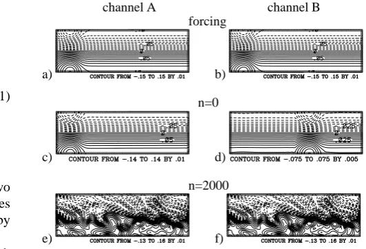
FIGURE 1. Fig. 1. Streamfunction (in units of 1.48×10⁹m2s−1) describing the forcingψ∗(a, b), and the evolving flowψ (c–f), in a parallel channel model with bidirectional coupling of medium scale modes for which|kx|>kx0=3 or|ky|>ky0=2, and|k|≤15, for the
indi-cated numbersnof time steps in a numerical integration. Parame-ters are as in Duane and Tribbia (2004). An average streamfunction for the two vertical layersi=1,2 is shown. Synchronization occurs by the last time shown (e, f), despite differing initial conditions.
geostrophic equation for potential vorticityq in a two-layer reentrant channel on aβ-plane:
Dqi
Dt ≡ ∂qi
∂t +J (ψi, qi)=Fi +Di (2)
where the layeri=1,2, ψ is streamfunction, and the Jaco-bianJ (ψ,·)=∂ψ
∂x ∂·
∂y−
∂ψ ∂y
∂·
∂x gives the advective contribution
to the Lagrangian derivativeD/Dt. Equation (2) states that potential vorticity is conserved on a moving parcel, except for forcingFi and dissipationDi. The discretized potential
vorticity is
qi =f0+βy+ ∇2ψi+Ri−2(ψ1−ψ2)(−1)i (3) wheref (x, y)is the vorticity due to the Earth’s rotation at each point(x, y),f0is the averagef in the channel,βis the constantdf/dy andRi is the Rossby radius of deformation
in each layer. The forcingF is a relaxation term designed to induce a jet-like flow near the beginning of the channel:
Fi=µ0(qi∗−qi) for qi∗ corresponding to the choice of ψ∗
shown in Fig. 1a. The dissipation termsD, boundary con-ditions, and other parameter values are given in Duane and Tribbia (2004).
Two models of the form (2), DqA/Dt=FA+DA and
DqB/Dt=FB+DB were coupled diffusively in one direc-tion by modifying one of the forcing terms:
604 G. S. Duane et al.: Synchronicity in predictive modelling
channel A channel B
n=40:
n=280:
FIGURE 2.
T A
B
A
A
B
A T
a)
b)
FIGURE 3.
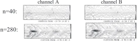
Fig. 2. Flow results as in Fig. 1, but with the inter-channel cou-pling restricted to the 10-local-bred-vector subspace as in Eq. (5). Synchronization is apparent by the time step shown.
The two sets of coefficientsµckandµextk were chosen to cou-ple the two channels in some medium range of wavenumbers and to force each channel only with the low wavenumber components of the background flow.
It was found that the two channels rapidly synchronize if only the medium scale modes are coupled (Fig. 1), starting from initial flow patterns that are arbitarily set equal to the forcing in one channel, and to a rather different pattern in the other channel. (Results are shown for bidirectional coupling defined by adding an equation forFkA analogous to Eq. 4. The synchronization behavior for coupling in just one di-rection is very similar.) With unididi-rectional coupling, the synchronization effects data assimilation from theAchannel into theBchannel.
One question about data assimilation that may be ad-dressed in the synchronization context concerns the defi-nition and minimum number of variables that must be as-similated to give adequate predictive skill. It has been ar-gued, for instance, that atmospheric dynamics is locally low-dimensional, and that a small number of locally selected bred vectors spans the effective state space in each local region (Patil et al., 2001). Bred vectors are commonly used to spec-ify likely directions of forecast error (Toth and Kalnay, 1993, 1997).
If Patil et al. (2001)’s argument about low “BV-dimension” is correct, then it should only be necessary to couple two channels in the subspace defined by the properly chosen bred vectors, in each local region, to synchronize the two chan-nels. That is, it should be possible to replace Eq. (4) by
FB(x, y)=µBVX i
[(qA−qB)·bi]kbi(x, y)+FBext(x, y) (5)
for(x, y)∈rk, where thebi fori=1...10 are an orthonormal
set of vectors formed from ten bred vectors Bi by
Gram-Schmidt orthogonalization in each local region separately. That is, the bred vectorsBi are first computed globally for
the channel as a whole, as in Toth and Kalnay (1997). Then, the channel is divided rectangularly into a 20×16 patch-work of local regionsrk k=1...320. The set of vectorsbi is
formed fromBi by Gram-Schmidt orthogonalization of the
setBi(x, y):(x, y)∈rk for eachrk and concatenating the
re-sulting vectors over all regions. The dot product in brackets in Eq. (5) is computed separately for each local region: [v·w]k ≡ X
(x,y)∈rk
v(x, y)w(x, y) (6)
so that 320×10=3200 independent coefficients [(qA −
qB)·bi]k are computed at each instant of time. Thus
[bi·bj]k=δij for allk. The overall coupling strength is given
by µBV, and the external forcing by the jet is defined by
FkBext≡µextk [qk∗−qkB]as before.
It is found that two channels coupled in a truncated bred vector basis according to Eq. (5) do synchronize, as illus-trated in Fig. 2, and do not synchronize with fewer indepen-dent regions or if fewer bred vectors are used to define the coupling subspace. The total number of independent coef-ficients, however, is comparable to or larger than the total number of Fourier components in the mid-range of scales that was seen to be effective for synchronization in the cou-pling scheme (4).
The lesson is that the synchronization phenomenon does not appear to be very sensitive to the detailed choice of cou-pling subspace. A similar conclusion was reached by Yang et al. (2004) for synchronizing Lorenz systems. Those authors obtained only small improvement by using bred vectors or singular vectors instead of single-variable coupling. In the present case of spatially extended models, it seems that any basis that captures the essential physical phenomena in each local region, phenomena that can be described in terms of a middle range of scales, is adequate for synchronization and hence for data assimilation.
2.3 Data assimilation
Standard data assimilation, unlike synchronization, estimates the current state xT∈Rn of one system, “truth”, from the state of a model systemxB∈Rn, combined with noisy
obser-vations of truth. The best estimate of truth is the “analysis”
xA, which is the state that minimizes error as compared to
all possible linear combinations of observations and model. That is
xA≡xB+3(xobs−xB) (7)
minimizes the analysis error<(xA−xT)2>for a stochastic
distribution given by xobs=xT+ξ whereξ is observational
noise, for properly chosenn×ngain matrix3. The standard methods to be considered in this paper correspond to specific forms for the generally time-dependent matrix3.
The simple method known as 3dVar uses a time-independent3that is based on the time-averaged statistical properties of the observational noise and the resulting fore-cast error. Let the matrix
R≡<ξ ξT >=< (xobs−xT)(xobs−xT)T > (8)
be the observation error covariance, and the matrix
be the “background” error covariance, describing the devia-tion of the model state from the true state. If both covariance matrices are assumed to be constant in time, then the optimal linear combination of background and observations is:
xA=R(R+B)−1xB+B(R+B)−1xobs (10)
The formula (10), which simply states that observations are weighted more heavily when background error is greater and conversely, defines the 3dVar method in practical data as-similation, based on empirical estimates of R and B. The 4dVar method, which will not be considered here, general-izes Eq. (10) to estimate a short history of true states from a corresponding short history of observations.
The Kalman filtering method, that is popular for a vari-ety of tracking problems, uses the dynamics of the model to update the background error covariance B sequentially. The analysis at each assimilation cycleiis:
xiA=R(R+Bi)−1xBi +Bi(R+Bi)−1xiobs (11)
where the backgroundxiB is formed from the previous anal-ysisxiA−1simply by running the modelM:Rn→Rn
xiB=Mi−1→i(xiA−1) (12)
as is done in 3dVar. But now the background error is updated according to
Bi =Mi−1→iAi−1MTi−1→i +Q (13)
where A is the analysis error covariance A≡<(xA−xT)(xA−xT)T>, given conveniently by A−1=B−1+R−1. The matrix M is the tangent linear model given by
Mab≡
∂Mb
∂xa
x=x
A
(14) The update formula (13) gives the minimum analysis error
<(xA−xT)2>=T rA at each cycle. The term Q is the
covari-ance of the error in the model itself, as discussed in Sect. 4.
3 Comparison of synchronization with standard meth-ods of data assimilation
3.1 Optimal coupling for synchronization of stochastic dif-ferential equations
To compare synchronization to standard data assimilation, we inquire as to the coupling that is optimal for synchroniza-tion, so that this coupling can be compared to the gain matrix used in the standard 3dVar and Kalman filtering schemes. The general form of coupling of truth to model that we con-sider in this section is given by a system of stochastic differ-ential equations:
˙
xT =f (xT)
˙
xB=f (xB)+C(xT −xB+ξ) (15)
where true statexT∈Rnand the model statexB∈Rnevolve
according to the same dynamics, given byf, and where the noise ξ in the coupling (observation) channel is the only source of stochasticity. The form (15) is meant to include dynamicsf described by partial differential equations, as in the last section. The system is assumed to reach an equi-librium probability distribution, centered on the synchro-nization manifold xB=xT. The goal is to choose a
time-dependent matrix C so as to minimize the spread of the dis-tribution.
Note that if C is a projection matrix, or a multiple of the identity, then Eq. (15) effects a form of nudging. But for arbitrary C, the scheme is much more general. Indeed, continuous-time generalizations of 3DVar and Kalman filter-ing can be put in the form (15).
Let us assume that the dynamics vary slowly in state space, so that the Jacobian F≡Df, at a given instant, is the same for the two systems
Df (xB)=Df (xT) (16)
where terms ofO(xB−xT)are ignored. Then the difference between the two Eqs. (15), in a linearized approximation, is ˙
e=Fe−Ce+Cξ (17)
wheree≡xB−xT is the synchronization error.
The stochastic differential equation (17) implies a de-terministic partial differential equation, the Fokker-Planck equation, for the probability distributionρ(e):
∂ρ
∂t + ∇e· [ρ(F−C)e] =
1
2δ∇e·(CRC
T∇
eρ) (18)
where R=<ξ ξT>is the observation error covariance matrix, andδ is a time-scale characteristic of the noise, analogous to the discrete time between molecular kicks in a Brownian motion process that is represented as a continuous process in Einstein’s well known treatment. Equation (18) states that the local change inρis given by the divergence of a proba-bility currentρ(F−C)eexcept for random “kicks” due to the stochastic term.
The PDF can be taken to have the Gaussian form
ρ=Nexp(−eTKe), where the matrix K is the inverse spread, andN is a normalization factor, chosen so that Rρdne=1. For background error covariance B, K=(2B)−1. In the one-dimensional case,n=1, whereCandKare scalars, substitu-tion of the Gaussian form in Eq. (18), for the stasubstitu-tionary case where∂ρ/∂t=0 yields:
2B(C−F )=δRC2 (19)
SolvingdB/dC=0, it is readily seen thatBis minimized (K
is maximized) whenC=2F=(1/δ)B/R.
In the multidimensional case,n>1, the relation (19) gen-eralizes to the fluctuation-dissipation relation
606 G. S. Duane et al.: Synchronicity in predictive modelling
channel A
channel B
n=40:
n=280:
FIGURE 2.
T A
B
A
A
B
A T
a)
b)
FIGURE 3.
Fig. 3. An analysis cycle, with trajectories shown for the true state “T”, the model evolving from the initial analysis “A” to the next forecast, or background “B”, and an alternative model run (dot-ted line) starting from an inferior “analysis” that is further from the initial truth. In the case (a) whereDf (xT)=Df (xA), then a worse analyis will always produce a worse forecast, but in the gen-eral case (b) whereDf (xT)6=Df (xA), nonlinearities may allow a
worse analysis to evolve to a better forecast (the trajectories do not actually cross).
that can be obtained directly from the stochastic differential equation (17) by a standard proof that is reproduced in Ap-pendix A. B can then be minimized element-wise. Differen-tiating the matrix equation (20) with respect to the elements of C, we find
dB(C−F)T +B(dC)T +(dC)B+(C−F)dB
=δ[(dC)RCT +CR(dC)T] (21) where the matrixdC represents a set of arbitrary increments in the elements of C, and the matrixdB represents the re-sulting increments in the elements of B. SettingdB=0, we have
[B−δCR](dC)T +(dC)[B−δRCT] =0 (22) Since the matrices B and R are each symmetric, the two terms in Eq. (22) are transposes of one another. It is eas-ily shown that the vanishing of their sum, for arbitrarydC, implies the vanishing of the factors in brackets in Eq. (22). Therefore C=(1/δ)BR−1, as in the 1D case.
3.2 Optimal synchronization vs. least-squares data assimi-lation
Turning now to the standard methods, so that a comparison can be made, it is recalled that the analysisxA after each
cycle is given by:
xA=R(R+B)−1xB+B(R+B)−1xobs
=xB+B(R+B)−1(xobs−xB) (23)
In 3dVar, the background error covariance matrix B is fixed; in Kalman filtering it is updated after each cycle using the linearized dynamics. The background for the next cycle is computed from the previous analysis by integrating the dy-namical equations:
xnB+1=xnA+τf (xnA) (24)
where τ is the time interval between successive analyses. Thus the forecasts satisfy a difference equation:
xnB+1=xBn +B(R+B)−1(xnobs−xnB)+τf (xnA) (25) We model the discrete process as a continuous process in which analysis and forecast are the same:
˙
xB=f (xB)+1/τB(B+R)−1(xT −xB+ξ)
+O[(B(B+R)−1)2] (26) using the white noiseξ to represent the difference between observationxobs and truthxT. The continuous
approxima-tion is valid so long asf varies slowly on the time-scaleτ. It is seen that when background error is small compared to observation error, the higher order termsO[(B(B+R)−1)2] can be neglected and the optimal coupling C=1/δBR−1is just the form that appears in the continuous data assimila-tion equaassimila-tion (26), forδ=τ. Thus under the linear assump-tion thatDf (xB)=Df (xT), the synchronization approach is
equivalent to 3dVar in the case of constant background error, and to Kalman filtering if background error is dynamically updated over time. The equivalence can also be shown for an exact description of the discrete analysis cycle, by comparing it to a coupled pair of synchronized maps. See Appendix B.
The equivalence between synchronization and standard methods in the linear case actually follows easily from a comparison of the optimization principles that define the two approaches. In the standard approaches, the form (23) min-imizes the expected value of(xA−xT)2, as compared to all
other linear combinations ofxobsandxB. But if double
lin-earization (16) holds then the minimization of<(xA−xT)2>
implies the minimization of <(xB−xT)2> at any future
time.
To see this, first consider the background error after a pe-riod of timeτ, just before the next analysis, as in Fig. 3a. If double linearization (16) holds, then this projected back-ground error is related to the initial analysis error by
e(t )=T
exp
Z t
to
F(t0)dt0
e(to)≡Me(to) (27)
where the notationT before the expression in brackets de-notes time-ordering. The expectations are related by B=<e(t )eT(t )>=M<e(to)eT(to)>MT=MAMT (28)
If we consider a more general “analysis”x3A formed from a general linear combination of forecast and observations
and compute a general “analysis error covariance” A3≡<(x3A−xT)(x3A−xT)T> accordingly, we seek to
minimize the traceT rA3=<(x3A−xT)2>. But it is readily
shown that a solution3of d3T rA3 =0 is also a solution ofd3T rM(t )A3MT(t )=0 for 0<t≤τ. (The operator “d3” produces a matrix with elements that are the derivatives of the argument with respect to the corresponding elements of
3.) Thus the best analysis gives the best forecast just prior to the next analysis. It is then readily seen that such a forecast will also give the best subsequent analysis and so on.
In the fully nonlinear case Df (xB)6=Df (xT), the best
analysis may not give the best forecast, as illustrated schematically in Fig. 3b. In this more general situation, the optimal coupling scheme for synchronization may dif-fer from that used in standard data assimilation methods. As a thought experiment, imagine a dynamical system that suddenly switches between two different dynamical regimes, given by different sets of equations, e.g. a 3-variable system that switches between Lorenz and Rossler dynamics, at reg-ular intervals. If the period between switches is long enough, a Kalman filter will take a little time to adjust the coupling to the new dynamics after each switch. This is a sub-optimal ar-rangement. The optimal arrangement would switch the cou-pling scheme completely each time the dynamics switches.
A version of this thought experiment, realized numeri-cally, is depicted in Fig. 4, using a non-autonomous three-variable system that switches, at periodic intervals 1, be-tween Lorenz dynamics and the same dynamics with the roles ofXandZreversed:
˙
X=σ (Y−X)
˙
Y =ρX−Y −XZ
˙
Z = −βZ+XY
ifn1≤t < (n+1/2)1 (n∈Z+)
(30) ˙
X= −βX+ZY
˙
Y =ρZ−Y −ZX
˙
Z =σ (Y−Z)
if(n+1/2)1≤t < (n+1)1
Synchronization of a master-slave pair of such systems was effected using coupling in theXandY variables, and alter-nately in theZandY variables, combinations known to be effective for the Lorenz system and the “reversed Lorenz” system, respectively:
˙
X1=σ (Y1−X1)+k(X−X1) ˙
Y1 =ρX1−Y1−X1Z1+k(Y −Y1) ˙
Z1= −βZ1+X1Y1
ifn1≤t < (n+1/2)1
(31) ˙
X1= −βX1+Z1Y1 ˙
Y1 =ρZ1−Y1−Z1X1+k(Y −Y1) ˙
Z1=σ (Y1−Z1)+k(Z−Z1)
a)
0 200 400 600 800 1000 1200 1400 1600 0
1 2 3 4 5 6 7 8 9 10
time
error
lorenz reversed lorenz
lorenz reversed lorenz
lorenz reversed lorenz
lorenz reversed lorenz
b)
0 200 400 600 800 1000 1200 1400 1600 0
1 2 3 4 5 6 7 8 9 10
time
error
lorenz reversed lorenz
lorenz reversed lorenz
lorenz reversed lorenz
lorenz reversed lorenz
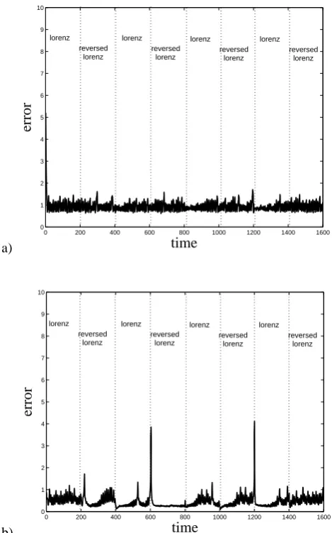
FIGURE 4. Fig. 4. Synchronization error between two copies of the alternat-ing Lorenz system (30), with standard Lorenz parameters and pe-riod1=400, coupled in two ways: (a) by simply alternating xy-coupling and zy-xy-coupling (31), with xy-coupling strengthk=140 and (b) by Kalman filtering with algorithm and parameters as in (Yang et al., 2004), except with low values of the covariance inflation fac-tor 1+δ=1.05 and of the standard deviationµ=0.025 of the random perturbations added to the analysis error covariance. The average error for 100 realizations of the stochastic process, all with the same initial conditions, is plotted in each panel. Runge-Kutta numerical integration was performed with stepsize1t=0.01. Time is shown in units equal to.08 in the nondimensional units of Eq. (31). Obser-vations were assimilated every eight time steps in the Kalman filter algorithm; the coupling term in Eq. (31) was analogously turned on only every eight time steps. The Kalman filtering algorithm gives lower error on the average, but there are some desynchroniza-tion bursts at times of regime transidesynchroniza-tions (dotted lines) between the Lorenz and “reversed Lorenz” phases.
if(n+1/2)1≤t < (n+1)1
608 G. S. Duane et al.: Synchronicity in predictive modelling byX1, Y1, Z1, based on “observations” of theX, Y, Z
sys-tem. It is seen that the Kalman filter approach (Fig. 4b) gives bursts of desynchronization just after the transitions, as expected, unlike the coupling (31) (Fig. 4a), although the Kalman filter performance is better on the average. (The plots in Fig. 4 are averages over a large number of realiza-tions of the stochastic process. Each realization is based on exactly the same master system trajectory. The desyn-chronization phenomenon occurs when the Lorenz/reversed Lorenz transition takes place at certain points on the master system attractor, but not when it takes place at other points.) There are several lessons to be learned from this extreme and somewhat artificial example. First, the optimal synchro-nization scheme, with time-varying coupling, would reduce both the average error and the bursting phenomenon. That would be the ideal way to do data assimilation. But sec-ond, the Kalman filtering approach is almost always better than any of the coupling algorithms described in the synchro-nization literature. Specifically, the bursts (corresponding to “catastrophes” in the data assimilation literature) are short-lived even in this extreme example, lasting for only one or two time steps.
In the geophysical realm, effective non-autonomy is com-mon, as with phenomena influenced by the diurnal or annual cycles for example. More generally, the highly nonlinear re-gions of phase space where the assumption (16) fails, and the optimality of the Kalman filter is expected to break down correspond to regime transitions. It is in such regions, that typically occupy small volumes of phase space, where the synchronization approach is expected to improve on standard methods to a small degree.
4 Synchronization vs. data assimilation for strongly nonlinear dynamics
In a region of state space where nonlinearities are strong and Eq. (16) fails, the prognostic equation for error (17) must be extended to incorporate nonlinearities. Additionally, model error due to processes on small scales that escape the digi-tal representation should be considered. While errors in the parameters or the equations for the explicit degrees of free-dom require deterministic corrections, the unresolved scales, assumed dynamically independent, can only be represented stochastically. The physical system is governed by:
˙
xT =f (xT)−ξM (32)
in place of Eq. (15a), whereξM is model error, with covari-ance Q≡<ξMξTM>. The error equation (17) becomes ˙
e=(F−C)e+Ge2+He3+Cξ+ξM (33)
where we have included terms up to cubic order ine, with
H <0 to prevent divergent error growth for large||e||. In the multi-dimensional case, Eq. (33) is shorthand for a tensor equation in which G andH are tensors of rank three and
rank four (and the restrictions onH are more complex). In the one-dimensional case, which we shall analyze here, G
andH are scalars.
The Fokker-Planck equation is now:
∂ρ
∂t + ∇e· {ρ[(F−C)e+Ge
2+H e3]}
= 1
2δ∇e· [(CRC
T +Q)∇
eρ] (34)
Using the ansatz for the PDFρ:
ρ(e)=Nexp(−Ke2−Le3−Me4) (35) with a normalization factor N = [R∞
−∞de exp(−Ke
2 −
Le3−Me4)]−1, we obtain from Eq. (34) the following rela-tions between the dynamical parameters and the PDF param-eters:
F −C= 1 2τ (C
2R+Q)(−2K)
G= 1 2τ (C
2R+Q)(−3L) (36)
H = 1 2τ (C
2R+Q)(−4M)
The goal is to minimize the background error:
B(K, L, M)=
R∞
−∞de e
2exp(−Ke2−Le3−Me4)
R∞
−∞de exp(−Ke2−Le3−Me4)
. (37) Using Eq. (36) to express the arguments of B
in terms of the dynamical parameters, we find
B(K, L, M)=B(K(C), L(C), M(C))≡B(C), and can seek the value ofC that minimizesB, for fixed dynamical parametersF, G, H.
For grounding in choosing appropriate parameter values, one might consider the nonlinearities of typical systems in geophysical fluid dynamics. The parameters G and H
can be taken from a Taylor expansion of the model sys-tem dynamics about the true state. That is, the expansion
f (y)=f (x)+ef0(x)+1 2e
2f00(x)+1 6e
3f000(x), for x = x
T,
y = xB, impliesG=1 2f
00(x)andH=1 6f
000(x), from which
(33) follows, noting (15). But then the prognostic equation for the true system can be similarly expanded aboutx=xo:
˙
x=f (xo)+(x−xo)F+(x−xo)2G+(x−xo)3H (38)
Suppose the true system (38) describes motion in a double-well potential with the central fixed point atx=xo, so that
f (xo)=0. It is at such points, e.g. the central fixed point in
a)
-3 -2 -1 1 2 3 x
-1.5 -1 -0.5 0.5 1 1.5
f
-d1 d2
b) 1.25 1.5 1.75 2.25 2.5 2.75 3 C 0.16
0.17 0.18
B
c)-1 -0.5 0.5 1 e 0.2
0.4 0.6 0.8
d)
1.25 1.5 1.75 2.25 2.5 2.75 3 C
0.021 0.022 0.023 0.024
B
FIGURE 5.
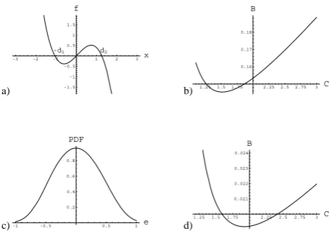
Fig. 5. For a true systemx˙=f (x), withf defined by (38) describ-ing a two-well potential aboutx=xo = 0, (a), background error
Bis plotted against coupling strengthCfor bimodality parameters
d1=1.06, d2=1.26, observation error R=1 and inter-observation
timeτ=0.1 (b). Although the distribution of true states is bimodal, the error distributionρ(e)is unimodal (c). B vs.C for a shorter inter-observation timeτ=0.01 (d) gives a covariance inflation fac-tor near unity (see text).
Matching the gross structure of the two-well potential to the gross structure of the Lorenz ’63 or Lorenz ’84 systems, one can find values ofGandH, that will give the correct distances between the central fixed point and the two out-lying fixed points, respectively. For the Lorenz ’84 system, these distances ared1=1.06 andd2=1.26 respectively. The prognostic equation for error (33) has fixed points in the de-sired positions iffG=.15 andH=−.75, in a re-scaled time coordinate for whichF=1.
For the perfect model case, Q=0, the function B(C) is then found numerically to have the form plotted in Fig. 5b, with a distinct optimum at B=0.15, C=1.5, where the inter-observation timeτ=0.1 (6 h in dimensional units) is chosen to be an order of magnitude smaller than the dynamical time scaleF−1and we assume a large observation errorR=1, of the same order as the typical displacement ofxabout the as-sumed unstable fixed point. Note that although the true state of the system is distributed bimodally, the distribution (35) of synchronization errorρ(e)shown in Fig. 5c is unimodal, because of smearing by observational noise.
The coupling that gives optimal synchronization can again be compared with the coupling used in standard data assim-ilation, as for the linear case. In particular, one can ask whether the “covariance inflation” scheme that is used as an ad hoc adjustment in Kalman filtering (Anderson 2001) can reproduce theCvalues found to be optimal for synchroniza-tion. The form C=τ−1B(B+R)−1 is replaced by the ad-justed form
C= 1
τ
FB
FB+R (39)
Table 1. Covariance inflation factor vs. bimodality parameters d1, d2, for 50% model error in the resolved tendency.
d1
.75 1. 1.25 1.5 1.75 2.
.75 1.26 1.26 1.28 1.30 1.32 1.34 1. 1.26 1.23 1.23 1.25 1.27 1.29
d2 1.25 1.28 1.23 1.22 1.23 1.24 1.25
1.5 1.30 1.25 1.23 1.22 1.23 1.24 1.75 1.32 1.27 1.24 1.23 1.23 1.23 2. 1.34 1.29 1.25 1.24 1.23 1.23
whereF is the covariance inflation factor. For the example depicted in Fig. 5b, the optimal valueC=1.5 would be gen-erated by an inflation factorF=1.2.
The optimization problem was solved numerically with re-sults as plotted in Table 1 for a range of values of the bi-modality parametersd1andd2, giving dynamical parameters
G=1/d2−1/d1 andH=−1/(d1d2). Results are displayed for the case where the amplitude of model error in Eq. (32) is about 50% of the resolved tendencyx˙T, with the resulting
model error covarianceQ=0.04 approximately one-fourth of the background error covarianceB. The covariance inflation factors are remarkably constant over a wide range of param-eters and agree with typical values used in operational prac-tice.
For the range of bimodality parameters considered, the large stochastic model error makes little difference in the estimated covariance inflation factors, typically changing
F only by about ±0.001. Indeed, for the linear case (d1=d2=∞), the optimal coupling is still 1/δBR−1, as for a perfect model. The stochastic model error results in an extra constant termδQon the RHS of the Fluctuation-Dissipation Relation (20) that does not affect the derivatives in the sub-sequent optimization procedure. (However,Qdoes enter the prognostic equation (13) forB in the linear case, just as in Kalman filtering.)
As the inter-observation timeτ becomes smaller, B de-creases at the minimum point, and the form (39) implies a decreasing covariance inflation factor. For the caseτ=0.01 shown in Fig. 5d, the required factor is near unity. (Precisely,
610 G. S. Duane et al.: Synchronicity in predictive modelling would seem to address some of the same issues treated in this
section, and a comparison is warranted.
In the synchronization view, the values typically used for the covariance inflation factor in the presence of model non-linearity and stochastic model error are readily explained. Sampling error, as it affects estimates of background covari-anceB, is not treated here, but might be expected to enter in a similar way and not to substantially alter the conclusions of the optimal coupling analysis.
5 Concluding remarks: data assimilation as machine perception
That ad hoc covariance inflation factors used in operational practice can be explained naturally in the synchronization view of data assimilation suggests a deep relevance for that viewpoint. Nothing in the foregoing discussion of synchro-nization and data assimilation is limited to meteorological processes. In any situation in which a computational predic-tive model of a physical process receives a stream of new data as it is running, the synchronization of the physical process and the model is the true goal of any assimilation scheme. As suggested in the introduction, the philosophical basis for the proposed use of synchronization appears to be the idea of synchronicity as espoused by Jung and Pauli, originally in a psychological context.
While a weather-prediction model is not usually viewed as artificially intelligent software, it forms an internal rep-resentation of the external world as complex as that of any robot, albeit without the motor component. One could envi-sion augmenting the statistical data assimilation algorithms with rules to discriminate between good and bad observa-tions, and with rules to transform the observed data in com-plex ways based on the current model state. Neurobiological paradigms may guide the design of such artificially intelli-gent predictive systems. It is known that interneuronal syn-chronization across wide distances in the brain plays a role in the grouping of percepts that is a prerequisite to higher processing, and may even underlie consciousness (Strogatz, 2003; Von Der Malsburg and Schneider, 1986). These find-ings lend credibility to the suggestion that a synchronization principle is also fundamental to the relationship between the brain and the external world, and that synchronization should be a cornerstone in the design of a neuromorphic, artificially intelligent predictive model.
Machine learning might also be realized in the synchro-nization context, so as to correct for deterministic model error in the resolved degrees of freedom. By allowing model parameters to vary slowly, generalized synchroniza-tion would be transformed to more nearly identical synchro-nization. Indeed, parameter adaptation laws can be added to a synchronously coupled pair of systems so as to synchronize the parameters as well as the states. Parlitz (1996) showed for example that two unidirectionally coupled Lorenz systems
with different parameters: ˙
X=σ (Y−X)
˙
Y =ρX−Y −XZ
˙
Z= −βZ+XY
(40) ˙
X1=σ (Y−X1) ˙
Y1=ρ1X1−νY1−X1Z1+µ ˙
Z1= −βZ1+X1Y1
could be augmented with parameter adaptation rules: ˙
ρ1=(Y−Y1)X1 ˙
ν=(Y1−Y )Y1 (41)
˙
µ=Y−Y1
so that the Lorenz systems would synchronize, and addition-ally ρ1→ρ, ν→1, and µ→0. Note that parameters cease to adapt when the systems are perfectly synchronized with
Y−Y1=0. Generalizations to PDEs would allow model pa-rameters to automatically adapt. In complex cases, a stochas-tic component (in the parameters) might be necessary to al-low parameters to jump among multiple basins of attraction, most of which are sub-optimal. The stochastic approach could perhaps be extended to a genetic algorithm that would make random qualitative changes in the model as well, until synchronization is achieved.
The main competing approach to the tracking of reality by a predictive model is Kalman filtering, or generaliza-tions thereof that use Bayesian reasoning to estimate the cur-rent state. Further development of the optimal synchroniza-tion approaches to provide more refined modificasynchroniza-tions of the Kalman filter in select regions of state space will be of inter-est in any situation where a Kalman filter is used to track a highly nonlinear process.
Conversely, unidirectional synchronization can always be viewed as a data assimilation problem, by regarding the slave system as a “model” of the master. The synchronization properties of a bidirectionally coupled system can often be inferred from the study of a corresponding unidirectional configuration. The optimally modified Kalman filter that is needed for data assimilation will therefore also be useful for optimizing the synchronization of dynamical systems gener-ally.
Appendix A
Derivation of the fluctuation-dissipation relation for synchronously coupled differential equations with noise in the coupling channel
Consider the stochastic differential equation for synchroniza-tion error (17), rewritten as:
de
whereeis the synchronization error vector, F is a matrix rep-resenting the linearized dynamics, C is the coupling matrix, andξ is a time-dependent vector of white noise process sat-isfying<ξ(t )>=0 and
<ξ(t )ξT(t0) >=δRδ(t−t0) (A2) where R is the observation error covariance matrix andδis the time over which the physical noise decorrelates. The so-lution to Eq. (A1) is:
e(t )=e(F−C)te(0)+
Z t
0
dt0e(F−C)(t−t0)Cξ(t0) (A3) Thus the mean synchronization error is
<e(t ) >=e(F−C)te(0) (A4) and the synchronization error variance is
<[e(t )−e(F−C)te(0)][e(t )−e(F−C)te(0)]T >=
Z t
0
dt0
Z t
0
dt00e(F−C)(t−t0)C<ξ(t0)ξT(t00>CTe(F−C)T(t−t00) (A5) or
<e(t )eT(t ) >=e(F−C)te(0)eT(0)e(F−C)Tt +
Z t
0
dt0e(F−C)(t−t0)δCRCTe(F−C)T(t−t0) (A6) If C is chosen so that the system synchronizes, in the absence of noise, ast→∞, then the first term on the right hand sided of Eq. (A6) vanishes in this limit. The system with noise approaches a stationary state with<e>=0 and
<eeT >≡B=
Z ∞
0
dte(F−C)tδCRCTe(F−C)Tt (A7) Differentiating the integrand in Eq. (A7) with respect totand and using Eq. (A7) to simplify the resulting expression, we find
(F−C)B+B(F−C)T
=
Z ∞
0
dtd dt[e
(F−C)tδCRCTe(F−C)Tt]
= [e(F−C)tδCRCTe(F−C)Tt]
∞
0 (A8)
The last expression in brackets vanishes at the upper limit for the case of stable synchronization, so we have
(F−C)B+B(F−C)T = −δCRCT (A9) which is the fluctuation-dissipation relation (20).
Appendix B
Optimal coupling for synchronization of discrete-time maps
In Sects. 3.1 and 3.2, standard data assimilation was com-pared to optimal synchronization of differential equations by considering the continuous-time limit of the discrete analy-sis cycle. Instead, one can leave the analyanaly-sis cycle intact and compare it to a discrete-time version of optimal synchroniza-tion, i.e. to optimally synchronized maps.
We begin by deriving a fluctuation-dissipation relation (FDR) for stochastic difference equations. Consider the stochastic difference equation with additive noise,
x(n+1)=Fx(n)+ξ(n) <ξ(n)ξ(m)T >=Rδn,m,(B1)
wherex,ξ∈Rn, F, R aren×nmatrices, F is assumed to be stable, andξ is Gaussian white noise. One can prove by in-duction that the solution to this equation, with initial condi-tionx(p), is
x(n+1)=Fn+1−px(p)+
n
X
m=p
Fm−pξ(n+p−m) (B2)
We first wish to find the equilibrium covariance matrix
0=<xxT>. If the initial condition is in the infinite past then the equilibrium covariance is the covariance at any finite it-eration and it is convenient to choose itit-eration one. Since F is stable the initial condition is forgotten and we obtain:
x(1)=
∞
X
m=0
Fmξ(−m), (B3)
and then
0=
∞
X
m=0
FmRFmT. (B4)
One can then show that0satisfies the matrix FDR
F0FT −0+R=0. (B5)
Now consider a model that takes the analysis at stepnto a new background at stepn+1, given by a linear matrix M. That is,xB(n+1)=MxA(n). Also,xT(n+1)=MxT(n). SincexA(n)=xB(n)+B(B+R)−1(xobs(n)−xB(n)), where xobs=xT+ξ, we derive a difference equation fore≡xB−xT: e(n+1)=M(I−B(B+R)−1)e(n)+MB(B+R)−1ξ. (B6) For synchronously coupled maps, on the other hand, we have
e(n+1)=(M−C)e(n+1)+Cξ, (B7)
and with the FDR as derived above:
612 G. S. Duane et al.: Synchronicity in predictive modelling Differentiating the matrix equation (B8) with respect to the
elements of C, as in the continuous-time analysis, we find 0=(M−C)dB(M−C)T +(−dC)B(M−C)T
+(M−C)B(−dC)T −dB+dCRCT +CRdCT. (B9) We seek a matrix C for whichdB=0 for arbitrarydC, and thus
(−dC)[B(M−C)T −RCT]
+[(M−C)B−CR](−dC)T =0 (B10) for arbitrarydC. The two terms are transposes of one an-other, and it is easily shown, as in the continuous-time case, that the quantities in brackets must vanish. This gives the optimal matrix
C=MB(B+R)−1 (B11)
which upon substitution in Eq. (B7) reproduces the standard data assimilation form (B6), confirming the equivalence.
Acknowledgements. The authors thank S.-C. Yang for providing
software used as a basis for the alternating Lorenz system experi-ment. The National Center for Atmospheric Research is sponsored by the National Science Foundation. This work was supported under NSF Grant 0327929.
Edited by: M. Thiel Reviewed by: two referees
References
Afraimovich, V. S., Verichev, N. N., and Rabinovich, M. I.: Stochastic synchronization of oscillation in dissipative systems, Radiophys. Quantum Electron., 29, 795–803, 1986.
Anderson, J. L.: An ensemble adjustment Kalman filter for data assimilation, Mon. Wea. Rev., 129, 2884–2903, 2001.
Anderson, J. L.: A local least-squares framework for ensemble fil-tering, Mon. Wea. Rev., 131, 634–642, 2003.
Corazza, M., Kalnay, E., Patil, D. J., Yang, S.-C., Morss, R., Cai, M., Szunyogh, I., Hunt, B. R., and Yorke, J. A.: Use of the breed-ing technique to estimate the structure of the analysis “errors of the day”, Nonlin. Processes Geophys., 10, 233–243, 2003, http://www.nonlin-processes-geophys.net/10/233/2003/. Ashwin, P., Buescu, J., and Stewart, I.: Bubbling of attractors and
synchronisation of chaotic oscillators, Phys. Lett. A, 193, 126– 139, 1994.
Baek, S. J., Hunt, B. R., Szunyogh, I., Zimin, A., and Ott, E.: Local-ized error bursts in estimating the state of spatiotemporal chaos, Chaos, 14, 1042–1049, 2004.
Corazza, M., Kalnay, E., Patil, D. J., Yang, S.-C., Morss, R., Cai, M., Szunyogh, I., Hunt, B. R., and Yorke, J. A.: Use of the breed-ing technique to estimate the structure of the analysis “errors of the day”, Nonlin. Processes Geophys., 10, 233–243, 2003, http://www.nonlin-processes-geophys.net/10/233/2003/. Duane, G. S.: Synchronized chaos in extended systems and
meteo-rological teleconnections, Phys. Rev. E, 56, 6475–6493, 1997.
Duane, G. S.: Synchronized chaos in climate dynamics, in: Proc. 7th Experimental Chaos Conference, edited by: In, V., Ko-carev, L., Carroll, T. L., et al., AIP Conference Proceedings 676, Melville, New York, 115–126, 2003.
Duane, G. S. and Tribbia, J. J.: Synchronized chaos in geophysical fluid dynamics, Phys. Rev. Lett., 86, 4298–4301, 2001. Duane, G. S. and Tribbia, J. J.: Weak Atlantic-Pacific
telecon-nections as synchronized chaos, J. Atmos. Sci., 61, 2149–2168, 2004.
Evensen, G.: Sequential data assimilation with a non-linear quasi-geostrophic model using Monte Carlo methods to forecast error statistics, J. Geophys. Res., 99, 10 143–10 162, 1994.
Fujisaka, H. and Yamada, T.: Stability theory of synchronized mo-tion in coupled-oscillator systems, Prog. Theor. Phys., 69, 32–47, 1983.
Jung, C. G. and Pauli, W.: The interpretation of nature and the psy-che, Pantheon, New York, 1955.
Kocarev, L., Tasev, Z., and Parlitz, U.: Synchronizing spatiotem-poral chaos of partial differential equations, Phys. Rev. Lett., 79, 51–54, 1997.
Lorenz, E. N.: Deterministic nonperiodic flows, J. Atmos. Sci., 20, 130–141, 1963.
Lorenz, E. N.: Irregularity – a fundamental property of the atmo-sphere, Tellus A, 36, 98–110, 1984.
Miller, R. N. and Ghil, M.: Advanced data assimilation in strongly nonlinear dynamical systems, J. Atmos. Sci., 51, 1037–1056, 1994.
Parlitz, U.: Estimating model parameters from time series by au-tosynchronization, Phys. Rev. Lett., 76, 1232–1235, 1996. Patil, D. J., Hunt, B. R., Kalnay, E., Yorke, J. A., and Ott, E.: Local
low dimensionality of atmospheric dynamics, Phys. Rev. Lett., 86, 5878–5881, 2001.
Pecora, L. M. and Carroll, T. L.: Synchronization in chaotic sys-tems, Phys. Rev. Lett., 64, 821–824, 1990.
Pecora, L. M., Carroll, T. L., Johnson, G. A., Mar, D. J., and Heagy, J. F.: Fundamentals of synchronization in chaotic systems, con-cepts, and applications, Chaos, 7, 520–543, 1997.
Rulkov, N. F., Sushchik, M. M., and Tsimring, L. S.: Generalized synchronization of chaos in directionally coupled chaotic sys-tems, Phys. Rev. E, 51, 980–994, 1995.
So, P., Ott, E., and Dayawansa, W. P.: Observing chaos – deducing and tracking the state of a chaotic system from limited observa-tion, Phys. Rev. E, 49, 2650–2660, 1994.
Strogatz, S. H.: Sync: The Emerging Science of Spontaneous Or-der, Theia, New York, 338 pp., 2003.
Toth, Z. and Kalnay, E.: Ensemble forecasting at NMC – the gener-ation of perturbgener-ations, Bull. Amer. Meteor. Soc., 74, 2317–2330, 1993.
Toth, Z. and Kalnay, E.: Ensemble forecasting at NCEP and the breeding method, Mon. Wea. Rev., 125, 3297–3319, 1997. Vautard, R., Legras, B., and D´equ´e, M.: On the source of
midlat-itude low-frequency variability. Part I: A statistical approach to persistence, J. Atmos. Sci., 45, 2811–2843, 1988.
Von Der Malsburg, C. and Schneider, W.: A neural cocktail-party processor, Biol. Cybernetics, 54, 29–40, 1986.